Inversion of the spherical means transform in corner-like domains by reduction to the classical Radon transform

Abstract

We consider an inverse problem arising in thermo-/photo- acoustic tomography that amounts to reconstructing a function $f$ from its circular or spherical means with the centers lying on a given measurement surface. (Equivalently, these means can be expressed through the solution $u(t,x)$ of the wave equation with the initial pressure equal to $f$.) An explicit solution of this inverse problem is obtained in 3D for the surface that is the boundary of an open octet, and in 2D for the case when the centers of integration circles lie on two rays starting at the origin and intersecting at the angle equal to $\pi/N$, $N=2,3,4,...$. Our formulas reconstruct the Radon projections of a function closely related to $f$, from the values of $u(t,x)$ on the measurement surface. Then, function $f$ can be found by inverting the Radon transform.

Keywords: photoacoustic tomography, thermoacoustic tomography, optoacoustic tomography, wave equation, spherical means, explicit inversion formulas

1 Introduction

Thermoacoustic tomography (TAT) [17, 41] and photo- or opto- acoustic tomography (PAT or OAT) [16, 34, 3] are based on the thermoacoustic effect: when a material is heated it expands. To perform measurements, a biological object is illuminated with a short electromagnetic pulse that heats the tissue and, through the resulting thermoacoustic expansion, generates an outgoing acoustic wave. Acoustic pressure is then measured by detectors placed on a surface (completely or partially) surrounding the object. The source reconstruction inverse problem of TAT/PAT/OAT consists in finding the initial pressure within the object from the measurements. This pressure is closely related to the blood content in the tissues, making these imaging modalities particularly effective for cancer detection and imaging of blood vessels.

Under the assumption that the speed of sound in the tissues is constant, for certain simple acquisition surfaces a solution of this inverse problem can be represented by explicit closed-form formulas. Such formulas are similar to the well-known filtration/backprojection formula in X-ray tomography; they allow one to compute the initial pressure by evaluating an explicit integro-differential operator at each node of a reconstruction grid. The existence and form of explicit inversion formulas are closely related to the shape of the data acquisition surface. For the simplest case of a planar surface, explicit formulas have been known for several decades [1, 9, 7]. The authors of [42] found a filtration/backprojection formula that is valid for a plane, a 3D sphere and an infinite 3D cylinder. In [11, 10, 21, 33] several different inversion formulas were derived for spherical acquisition surfaces in spaces of various dimensions. In [23] explicit reconstruction formulas were obtained for detectors placed on a surface of a cube (or square, in 2D) or on surfaces of certain other polygons and polyhedra. Several authors [38, 35, 28, 14] recently found explicit inversion formulas for the data measured from surfaces of an ellipse (in 2D) or an ellipsoid (in 3D) surrounding the object. These formulas can be further extended by continuity to an elliptic paraboloid or parabolic cylinder [29, 30]. Certain more complicated polynomial surfaces (including a paraboloid) were considered in [35], although not all of these surfaces are attractive from a practical point of view, as they would require surrounding the object by several layers of detectors. In addition to the explicit formulas, there exist several reconstruction algorithms (for closed acquisition surfaces) based on various series expansions  [31, 32, 22, 24, 13]. These techniques sometimes lead to very fast implementations (e.g.  [22, 24]); however, their efficient numerical implementation may require certain non-trivial computational skills.

In this paper we derive inversion formulas for acquisition schemes that use either linear arrays of point- or line- detectors, or two dimensional arrays of sensors partially surrounding the object. Several experimental setups motivate our research. For example, in [5], linear detectors were arranged in a corner-like assembly rotated along the object. Such a scheme requires inversion of series of 2D circular Radon transforms with centers located on two perpendicular rays. A similar 3D problem sometime arises when optically scanned planar glass plate is used as an acoustic detector, as done by researchers from University College London (see, for example, [6, 8]). The use of a single glass plate provides only a limited angle view of the object, leading to disappearance of some edges in the image. To eliminate such artifacts, one needs to repeat scanning with a detector repositioned to view the object at a different angle, or to add additional glass plates and/or acoustical mirrors. The methods of the present paper are applicable in the case of consecutive measurements. The acquisition scheme with multiple glass detectors may need to be modeled as a reverberating cavity due to multiple reflections of acoustic waves from the glass surfaces. The methods of the present paper are not applicable in such situation; instead, the reader is referred to [6, 8, 20, 15].

Recently, linear arrays of point-like piezoelectric detectors started to gain popularity due to their fast rate of acquisition (see [18, 26, 25]). Similarly to planar arrays, one such linear assembly yields only limited-angle measurements, and one has to either use mirrors (as is done in [25]), or to arrange several arrays around the object (reflections from linear arrays can be neglected due to their smaller cross-section).

In this paper we consider a 3D acquisition scheme where point detectors are located on the boundary of an infinite octant, and a similar 2D problem with detectors covering the boundary of an infinite angular sector with an opening angle $\pi/N$, $N=2,3,4,...$. In both cases it is assumed that reflection of acoustic waves from the detectors is either absent or negligible. Unlike many of inversion formulas mentioned above, the formulas we derive are not of a filtration/backprojection type. Instead, we obtain explicit expressions allowing one to recover from the measurements the classical Radon projections of the unknown initial pressure. The latter function then is easily reconstructed by application of the well-known inverse Radon transform.

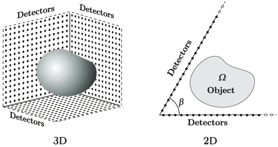
Figure 1: Acquisition geometry in 3D and 2D

2 Preliminaries

2.1 Formulation of the problem

We assume throughout the paper that the attenuation of acoustic waves is negligible, and that the speed of sound in the tissues is constant (and, thus, it can be set to 1 without loss of generality). This simplified model is acceptable in such important applications as breast imaging, and most of the formulas and algorithms mentioned in the Introduction are based on these assumptions. Then, the acoustic pressure $p(t,x)$ solves the following initial problem for the wave equation in the whole space $\mathbb{R}^{d},$ $d=3,$

$$\left\{\begin{array}[c]{c}p_{tt}=\Delta p,\text{ }x\in\mathbb{R}^{d},\quad t\in[0,\infty),\\ p(0,x)=f(x),\\ p_{t}(0,x)=0.\end{array}\right.$$ (1)

were the initial pressure of the acoustic wave $f(x)$ is the function we seek. It is assumed that $f(x)$ is finitely supported within the region of interest $\Omega,$ and that the point-wise measurements of $p(t,x)$ are done outside $\Omega.$ A very similar two-dimensional problem arises when linear integrating detectors are used for measurements (e.g., see [13]). For example, if a set of linear detectors parallel to vector $e_{3}=(0,0,1)$ is utilized, they measure integrals $I(t,x_{1},x_{2})$ of the pressure along lines parallel to $e_{3}$ and the problem consists in finding the initial distribution of these integrals $f(x)\equiv I(0,x_{1},x_{2})$. This problem can also be formulated in the form (1), with $d=2,$ with $p(t,x)$ replaced by $I(t,x_{1},x_{2}).$

Our goal is to reconstruct $f(x)$ from measurements of $p(t,x)$ made at all points of the measuring surface (or, in 2D, measuring curve). In 3D, as the measuring surface we will use the boundary $\partial Q$ of the first Cartesian octet $Q$ in $\mathbb{R}^{3}$:

$$Q\equiv\{x\in\mathbb{R}^{3}|x_{1}>0,x_{2}>0,x_{3}>0\}.$$ (2)

For the 2D problem the data $u(t,x)$ will be assumed known on the boundary of infinite angular segment $Q$ contained between the ray $\mathbb{R}^{+}\equiv\{(c,0)|\ c\geq 0\}$ and ray $\mathbb{R}_{\beta}^{+}\equiv\{(c\cos\beta,c\sin\beta)|\ c\geq 0\}$, where angle $\beta$ is to one of the values $\pi/N,$ $N=2,3,4,...$ . In this case the measuring curve $\partial Q$ is the union $\mathbb{R}^{+}\cup\mathbb{R}_{\beta}^{+}$. Figure 1 shows schematically the measuring sets in 2D and 3D. In both cases it is assumed that the support $\Omega$ of $f$ is properly contained in $Q.$

Thus, our ultimate goal is to find explicit reconstruction formulas expressing $f(x)$ through measured values $p(t,y),\quad y\in\partial Q,\quad t\in[0,\infty).$

2.2 Outline of the approach

Solution of the initial value problem (1) can be written as a convolution of $f$ with the time derivative of the retarded (or causal) Green’s function $G^{+}(t,x)$ of the wave equation in free space [40]:

$$p(t,y)=\frac{\partial}{\partial t}\int\limits_{\Omega}f(x)G^{+}(t,y-x)dx.$$ (3)

In 3D the above-mentioned Green’s function takes form

$$G_{(3D)}^{+}(t,x)=\frac{\delta(t-|x|)}{4\pi|x|},$$

where $\delta(t)$ is the Dirac’s delta function. In 2D

$$G_{(2D)}^{+}(t,x)=\left\{\begin{array}[c]{cc}\frac{1}{2\pi\sqrt{t^{2}-|x|^{2}}}&t>|x|,\\ 0&\text{otherwise}\end{array}\right..$$

The measurements $p(t,y)$ are just the values of the convolution (3) at points $y$ lying on $\partial Q.$ The time anti-derivative of the data $P(t,y)$ can be easily recovered from $p(t,y)$:

$$p(t,y)=\frac{\partial}{\partial t}P(t,y),\quad P(0,y)=0,\quad y\in\partial Q.$$

Function $P(t,y)$ is related to $\ f(x)$ by the convolution

$$P(t,y)=\int\limits_{\Omega}f(x)G^{+}(t,y-x)dx,\quad y\in\partial Q.$$

For notational convenience we extend $p(t,y)$ to negative values of $t$ by zero:

$$p(t,y)=0,\quad t\leq 0.$$ (4)

(With this convention equation (3) is valid for all $t\in\mathbb{R}$.)

Below we will also use the advanced free-space Green’s function $G^{-}(t,x)$ that allows one to solve wave equation backwards in time. It can be defined simply by reversing the sign in front of $t$:

$$G^{-}(t,x)=G^{+}(-t,x).$$

Consider now an integrable function $\varphi(t,y)$ defined on $\mathbb{R\times}\partial Q$, finitely supported in the first variable and decaying in $y$ fast enough so that the integral below converges absolutely. One can define a retarded single layer potential $u_{\varphi}^{+}(t,x)$ with density $\varphi(t,y)$ by the following equation [12, 39]:

$$u_{\varphi}^{+}(t,x) =\int\limits_{\partial Q}\int\limits_{-\infty}^{t-|y-x|}\varphi(\tau,y)G^{+}(t-\tau,y-x)d\tau dy$$

$$=\int\limits_{\partial Q}\int\limits_{|y-x|}^{\infty}\varphi(t-s,y)G^{+}(s,y-x)dsdy.$$

Similarly, an advanced single layer potential is given by the formula

$$u_{\varphi}^{-}(t,x) =\int\limits_{\partial Q}\int\limits_{-\infty}^{-|y-x|}\varphi(t-s,y)G^{-}(s,y-x)dsdy$$

$$=\int\limits_{\partial Q}\int\limits_{|y-x|}^{\infty}\varphi(t+s,y)G^{+}(s,y-x)dsdy.$$

Due to vanishing of $G^{+}(s,y-x)$ when $s<|y-x|,$ one can equivalently write

$$u_{\varphi}^{\pm}(t,x)=\int\limits_{\partial Q}\int\limits_{\mathbb{R}}\varphi(t\mp s,y)G^{+}(s,y-x)dsdy.$$

Our approach to the inverse problem in hand is based on the observation that the integral $<f,u_{\varphi}^{-}(0,\cdot)>$ defined as

$$<f,u_{\varphi}^{-}(0,\cdot)>\equiv\int\limits_{\Omega}f(x)u_{\varphi}^{-}(0,x)dx$$

can be easily reconstructed from the data $P(t,y)$:

$$\int\limits_{\Omega}f(x)u_{\varphi}^{-}(0,x)dx =\int\limits_{\Omega}f(x)\left[\int\limits_{\partial Q}\int\limits_{\mathbb{R}}\varphi(s,y)G^{+}(s,y-x)dsdy\right]dx$$

$$=\int\limits_{\partial Q}\int\limits_{\mathbb{R}}\varphi(s,y)\left[\int\limits_{\Omega}f(x)G^{+}(s,y-x)dx\right]dsdy$$

$$=\int\limits_{\partial Q}\int\limits_{\mathbb{R}}\varphi(s,y)P(s,y)dsdy.$$

This procedure can be repeated for a set of single layer potentials $u_{\varphi}^{-}(t,x)$ defined by different densities $\varphi.$ If these potentials evaluated at $\ t=0$ form some sort of a basis, the above integrals provide projections of $f$ on the basis elements, making it possible to reconstruct $f.$

Finding families of basis functions represented by single layer potentials is not necessarily easy, especially in unbounded domains. In general, certain solutions of the wave equation can be represented by a combination of a single- and double- layer potentials. For example, if $u(t,x)$ is a finitely supported in time solution of the wave equation in a bounded region $Q^{*}$ with a boundary $\partial Q^{*}$, then $u$ can be represented in the following form [12, 39]

$$u(t,x) =\int\limits_{\partial Q^{*}}\int\limits_{\mathbb{R}}\frac{\partial}{\partial n}u(t\mp s,y)G^{+}(s,y-x)dsdy$$

$$-\int\limits_{\partial Q^{*}}\int\limits_{\mathbb{R}}u(t\mp s,y)\frac{\partial}{\partial n}G^{+}(s,y-x)dsdy.$$

where second term is a double layer potential with density $u(\tau,y).$ Sign $\mp$ in the above equation indicates that $u(t,x)$ can be expressed through its boundary values (including the values of the normal derivative) either in the past, at the times $\,(t-s),$ or in the future (at the time values $t+s).$

However, for our purposes we need representations expressed only by a single potential supported on a boundary of a domain, and our domains are not bounded. In what follows we show that such representations can be obtained for certain combinations of delta-like plane waves. This will allow us to recover from the data the integrals of products of $f(x)$ with these functions; such integrals are related to the values of the Radon transform of $f(x)$. Then, $f(x)$ can be reconstructed by inverting the Radon transform.

3 Single layer representations

In this section we find single layer representations for certain combinations of plane waves.

3.1 2D case

Consider now a Coxeter cross, i.e. a set of $N$ straight lines passing through the origin, with the angle $\beta=\pi/N$ between any two adjacent lines; without loss of generality we assume that one of these lines coincides with $x_{1}$-axis. The boundary of the 2D angular segment $Q$ arising in the 2D formulation of our inverse problem (see Section 2.1) is a subset of this set of points. (For a discussion of injectivity of the spherical mean Radon transform with centers lying on a Coxeter cross we refer the reader to [2].)

3.1.1 An “odd” operator

In this section we define an operator that maps an arbitrary continuous function of $x\in\mathbb{R}^{2}$ into a function that is odd with respect to reflections about all the lines constituting the Coxeter cross.

Define a reflector $\mathfrak{R}$ mapping $x=(x_{1},x_{2})^{T}$ onto $\mathfrak{R}x=(x_{1},-x_{2})^{T},$ and a linear operator $\Upsilon_{\varphi}$ rotating any vector $x\in\mathbb{R}^{2}$  by the angle $\varphi$ counterclockwise. Obviously

$$\Upsilon_{2\beta}^{N}=\Upsilon_{2\beta}^{-N}=I$$ (5)

where $I$ is the identity transformation. Now, let us define an operator $O$ transforming a continuous function $h(x)$ into a continuous function $h_{O}(x)$ according to the following formula

$$h_{O}(x)=Oh(x)=\sum_{k=0}^{N-1}\left[h(\Upsilon_{2\beta}^{k}x)-h(\mathfrak{R}\Upsilon_{2\beta}^{k}x)\right].$$ (6)

It follows from (5) and (6) that $h_{O}(x)$ is invariant with respect to rotations by the angle $2\beta$

$$h_{O}(\Upsilon_{2\beta}x)=h_{O}(\Upsilon_{2\beta}^{-1}x)=h_{O}(x),$$

and, in general

$$h_{O}\left(\Upsilon_{2\beta}^{k}x\right)=h_{O}(x),\quad k\in\mathbb{Z}.$$ (7)

Further, we notice that due to (5)

$$\sum_{k=0}^{N-1}h(\mathfrak{R}\Upsilon_{2\beta}^{k}x)=\sum_{k=0}^{N-1}h(\mathfrak{R}\Upsilon_{2\beta}^{-k}x)=\sum_{k=0}^{N-1}h(\Upsilon_{2\beta}^{k}\mathfrak{R}x),$$ (8)

where the second equality is verified as follows. Each $x$ can be written as  $|x|\Upsilon_{\theta}e_{1}$, where $e_{1}=(1,0)^{T}$ and $\theta$ is some angle. Then

$$\mathfrak{R}\Upsilon_{2\beta}^{-k}x=\mathfrak{R}\Upsilon_{2\beta}^{-k}\left(|x|\Upsilon_{\theta}e_{1}\right)=|x|\mathfrak{R}\Upsilon_{(-2k\beta+\theta)}e_{1}=|x|\Upsilon_{(2k\beta-\theta)}e_{1}=\Upsilon_{2\beta}^{k}\mathfrak{R}x,$$

which proofs the second equality in (8). Therefore, operator $O$ (defined by equation (6)) admits an alternative representation

$$h_{O}(x)=Oh(x)=\sum_{k=0}^{N-1}\left[h(\Upsilon_{2\beta}^{k}x)-h(\Upsilon_{2\beta}^{k}\mathfrak{R}x)\right].$$ (9)

Since $\mathfrak{R}^{2}=I,$ it is immediately clear from (9) that

$$h_{O}(\mathfrak{R}x)=-h_{O}(x),$$

i.e., $h_{O}(x)$ is an odd function in $x_{2}$. Moreover, due to the rotation invariance (7), $h_{O}(x)$ is odd with respect to any line that is a rotation of the $x_{1}$ axis by the angle $2\beta k,$ $k\in\mathbb{\not Z}$, and

$$h_{O}(\mathfrak{R}\Upsilon_{2\beta}^{k}x)=-h_{O}(x),\quad k\in\mathbb{Z}.$$ (10)

One can also show that $h_{O}$ is odd with respect to any line that is a rotation of $x_{1}$-axis by the angle ($2k+1)\beta,$ $k\in\mathbb{Z}$. Let’s consider two points $c\Upsilon_{\alpha}\Upsilon_{\beta}e_{1}$ and $c\Upsilon_{-\alpha}\Upsilon_{\beta}e_{1}$ symmetric with respect to the line $t\Upsilon_{\beta}e_{1}$, $t\in(-\infty,\infty).$ Due to periodicity (equation (5)), $h_{O}$ admits yet another representation

$$h_{O}(x)=Oh(x)=\sum_{k=0}^{N-1}\left[h(\Upsilon_{2\beta}^{k}x)-h(\Upsilon_{2\beta}^{k+1}\mathfrak{R}x)\right].$$

Then

$$h_{O}(c\Upsilon_{\alpha}\Upsilon_{\beta}e_{1}) =\sum_{k=0}^{N-1}\left[h(c\Upsilon_{2\beta}^{k}x\Upsilon_{\alpha}\Upsilon_{\beta}e_{1})-h(c\Upsilon_{2\beta}^{k+1}\mathfrak{R}\Upsilon_{\alpha}\Upsilon_{\beta}e_{1})\right]$$

$$=\sum_{k=0}^{N-1}\left[h(c\Upsilon_{2\beta(k+1)+\alpha}e_{1})-h(c\Upsilon_{2\beta(k+1)-\alpha}e_{1})\right]=-h_{O}(c\Upsilon_{-\alpha}\Upsilon_{\beta}e_{1}).$$

Therefore, $h_{O}$ is odd with respect to a rotation of $x_{1}$-axis by the angle $\beta,$ and due to the $2\beta$-periodicity (equation (7)), it is odd with respect to a rotation of $x_{1}$-axis by the angle $(2k+1)\beta.$ Thus, we have proved the following

Proposition 1

Operator $O$ defined by equation (6) maps a continuous function into a continuous function that is odd with respect to reflections about each of the lines constituting the Coxeter cross.

Corollary 2

If $h_{O}(x)=Oh(x)$, then $h_{O}(x)$ vanishes on each of the lines constituting the Coxeter cross, and, in particular, on the boundary $\partial Q$ of segment $Q.$

Proposition 3

If support of $h(x)$ is contained within $Q,$ then restriction of $h_{O}$ to $Q$ coincides with $h,$ i.e.

$$h(x)=h_{O}(x),\quad\forall x\in Q.$$

Proof. If support of $h(x)$ is contained within $Q$, then each term in (6) that is not $h(x)$ itself, is supported within one of rotated and/or reflected versions of segment $Q$ not intersecting $Q$ itself.   

Proposition 4

Suppose $g(x)$ and $h(x)$ are continuous functions, one of them is compactly supported, with $g_{O}(x)=Og(x)$ and $h_{O}(x)=Oh(x).$ Then

$$\int\limits_{\mathbb{R}^{2}}g_{O}(x)h(x)dx=\int\limits_{\mathbb{R}^{2}}h_{O}(x)g(x)dx.$$

Proof. By using the definition of operator $O$ and interchanging the order of summation and integration one obtains

$$\int\limits_{\mathbb{R}^{2}}g_{O}(x)h(x)dx =\sum_{k=0}^{N-1}\int\limits_{\mathbb{R}^{2}}g(\Upsilon_{2\beta}^{k}x)h(x)dx-\sum_{k=0}^{N-1}\int\limits_{\mathbb{R}^{2}}g(\mathfrak{R}\Upsilon_{2\beta}^{k}x)h(x)dx$$

$$=\sum_{k=0}^{N-1}\int\limits_{\mathbb{R}^{2}}g(x)h(\Upsilon_{2\beta}^{-k}x)dx-\sum_{k=0}^{N-1}\int\limits_{\mathbb{R}^{2}}g(x)h(\mathfrak{R}\Upsilon_{2\beta}^{-k}x)dx$$

$$=\int\limits_{\mathbb{R}^{2}}g(x)\left(\sum_{k=0}^{N-1}\left[h(\Upsilon_{2\beta}^{-k}x)-h(\mathfrak{R}\Upsilon_{2\beta}^{-k}x)\right]\right)dx=$$

$$=\int\limits_{\mathbb{R}^{2}}g(x)\left(\sum_{k=0}^{N-1}\left[h(\Upsilon_{2\beta}^{k}x)-h(\mathfrak{R}\Upsilon_{2\beta}^{k}x)\right]\right)dx=\int\limits_{\mathbb{R}^{2}}h_{O}(x)g(x)dx,$$

where (5) was used on the last line.   

Finally, the following statement follows directly from (7) and (10).

Proposition 5

If $g(x)$ and $h(x)$ are continuous functions and $g(x)$ is compactly supported then

$$\int\limits_{\mathbb{R}^{2}}g(x)h_{O}\left(\Upsilon_{2\beta}^{k}x\right)dx =\int\limits_{\mathbb{R}^{2}}g(x)h_{O}(x)dx,$$

$$\int\limits_{\mathbb{R}^{2}}g(x)h_{O}\left(\Upsilon_{2\beta}^{k}\mathfrak{R}x\right)dx =-\int\limits_{\mathbb{R}^{2}}g(x)h_{O}\left(x\right)dx,\quad k\in\mathbb{Z}.$$

3.2 3D case

In the 3D version of our problem, region $Q$ is the first Cartesian octet $Q$ defined by equation (2).

3.2.1 An “odd” operator

In this section we define an operator that maps an arbitrary continuous function of 3D variable into function that is odd with respect to reflections about any of the three coordinate planes.

Let us define operators $\mathfrak{R}j,$ $j=1,2,3,$ reflecting any $x=(x_{1},x_{2},x_{3})^{T}$ with respect to the coordinate plane with the normal $e_{j}$:

$$\mathfrak{R}_{1}x =(-x_{1},x_{2},x_{3})^{T},$$

$$\mathfrak{R}_{2}x =(x_{1},-x_{2},x_{3})^{T},$$ (11)

$$\mathfrak{R}_{3}x =(x_{1},x_{2},-x_{3})^{T}.$$

It follows from the above definition that these reflectors commute.

We can now define an operator $O$ mapping continuous function $h(x)$ into function $h_{O}(x)$ odd with respect to reflections about each of the three coordinate planes$:$

$$h_{O}(x) =Oh(x)\equiv h(x)-h(\mathfrak{R}_{1}x)-h(\mathfrak{R}_{2}x)-h(\mathfrak{R}_{3}x)$$

$$+h(\mathfrak{R}_{2}\mathfrak{R}_{1}x)+h(\mathfrak{R}_{3}\mathfrak{R}_{1}x)+h(\mathfrak{R}_{3}\mathfrak{R}_{2}x)-h(\mathfrak{R}_{3}\mathfrak{R}_{2}\mathfrak{R}_{1}x).$$ (12)

Since operators $\mathfrak{R}j$ commute and are self-invertible, verifying that operator $O$ have the above-mentioned property is straightforward.

Proposition 6

Operator $O$ defined by equation (12) maps a continuous function into a continuous function that is odd with respect to reflections about each of the three coordinate planes.

Similarly, one proves

Proposition 7

If $h(x)$ is bounded and $h_{O}(x)=Oh(x)$ then

$$h_{O}\left(\mathfrak{R}_{i}x\right)=-h_{O}(x),\quad h_{O}\left(\mathfrak{R}_{i}\mathfrak{R}_{j}x\right)=h_{O}(x),\quad h_{O}\left(\mathfrak{R}_{i}\mathfrak{R}_{j}\mathfrak{R}_{k}x\right)=-h_{O}(x),\quad i,j,k\in\{1,2,3\}.$$

Corollary 8

If $h_{O}(x)=Oh(x)$, then $h_{O}(x)$ vanishes on each of the coordinate planes, in particular, on the boundary $\partial Q$ of the first octet $Q.$

Proposition 9

If support of $h(x)$ is contained within $Q,$ then restriction of $h_{O}$ to $Q$ coincides with $h,$ i.e.

$$h(x)=h_{O}(x),\quad\forall x\in Q.$$

Proposition 10

Suppose $g(x)$ and $h(x)$ are continuous functions, one of them is compactly supported, with $g_{O}(x)=Og(x)$ and $h_{O}(x)=Oh(x).$ Then

$$\int\limits_{\mathbb{R}^{3}}g_{O}(x)h(x)dx=\int\limits_{\mathbb{R}^{3}}h_{O}(x)g(x)dx.$$

The proof of the last proposition is similar to that of Proposition 4.

As a direct consequence of Proposition 7, one obtains

Proposition 11

If $g(x)$ and $h(x)$ are continuous functions, and $g(x)$ is compactly supported, then

$$\int\limits_{\mathbb{R}^{3}}g(x)h_{O}\left(\mathfrak{R}_{i}\right)dx =-\int\limits_{\mathbb{R}^{3}}g(x)h_{O}(x)dx,$$

$$\int\limits_{\mathbb{R}^{3}}g(x)h_{O}\left(\mathfrak{R}_{i}\mathfrak{R}_{j}x\right) =\int\limits_{\mathbb{R}^{3}}g(x)h_{O}(x)dx,$$

$$\int\limits_{\mathbb{R}^{3}}g(x)h_{O}\left(\mathfrak{R}_{i}\mathfrak{R}_{j}\mathfrak{R}_{k}x\right) =-\int\limits_{\mathbb{R}^{3}}g(x)h_{O}(x)dx,\quad i,j,k\in\{1,2,3\}.$$

3.3 Waves represented by single layer potentials

3.3.1 Odd combinations of waves

Consider a non-negative, infinitely smooth, even function $\eta\left(t\right)$  defined on $\mathbb{R}$, compactly supported with all its derivatives on $(-1,1)$, and such that $\int_{-1}^{1}\eta dt=1$. Define scaled function $\eta_{\varepsilon}(t)$ by the formula

$$\eta_{\varepsilon}(t)=\frac{1}{\varepsilon}\eta\left(\frac{1}{\varepsilon}t\right).$$

Family of functions $\eta_{\varepsilon}(t)$ is delta-approximating, in the sense of distributions:

$$\lim_{\varepsilon\rightarrow 0}\eta_{\varepsilon}(t)=\delta(t).$$ (13)

Now, let us consider a plane wave $u_{\varepsilon}(t,x)$ defined by the equation

$$u_{\varepsilon,\omega}(t,x)=\eta_{\varepsilon}\left(t-x\cdot\omega\right),$$

where $\omega$ is a unit vector defining the direction of propagation of such a wave. It is easy to check that $u_{\varepsilon}(t,x)$ is a solution of the wave equation in the whole space $\mathbb{R}^{d}$:

$$\Delta u_{\varepsilon,\omega}=\frac{\partial^{2}}{\partial t^{2}}u_{\varepsilon,\omega},\qquad x\in\mathbb{R}^{d},\quad t\in\mathbb{R},$$

and that, in the limit $\varepsilon\rightarrow 0,$ $u_{\varepsilon,\omega}$ approximates a delta-wave

$$\lim_{\varepsilon\rightarrow 0}u_{\varepsilon,\omega}(t,x)=\delta(t-x\cdot\omega).$$

Let us now use the operator $O$ introduced in the previous sections and define the following combination of plane waves:

$$U_{\varepsilon,\omega}(t,x)=Ou_{\varepsilon,\omega}(t,x).$$ (14)

To simplify the notation, within this section we will suppress the subscripts and denote this function by $U(t,x).$ Function $U(t,x)$ consists of the plane wave $u_{\varepsilon,\omega}(t,x)$ together with its reflections and (in 2D case) rotations, selected in such a way that it is odd with respect to a set of lines (or planes) containing the boundary of $\partial Q.$ Thus,

$$U(t,x)=0,\qquad\forall x\in\partial Q,\quad\forall t\in\mathbb{R}.$$

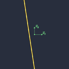
(a) Wave $u_{\varepsilon,\omega}(t,x)$

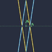
(b) $U(t,x)$, case $N=2$

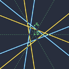
(c) $U(t,x)$, case $N=3$

Figure 2: Constructing $U(t,x)$ from $u_{\varepsilon,\omega}(t,x)$ in the cases $N=2$ and $N=3$. The dashed line shows the lines of the Coxeter cross; $U(t,x)$ is odd with respect to these lines

From now on, let us assume that vector $\omega$ is pointing strictly inside $Q$. In the 2D case the operator $O$ is defined by equation (6).

Apply it to $u_{\varepsilon,\omega}(t,x)$:

$$U(t,x) =Ou_{\varepsilon,\omega}(t,x)=$$

$$=\sum_{k=0}^{N-1}\left[\eta_{\varepsilon}\left(t-\Upsilon_{2\beta}^{k}x\cdot\omega\right)-\eta_{\varepsilon}\left(t-\mathfrak{R}\Upsilon_{2\beta}^{k}x\cdot\omega\right)\right]$$

$$=\sum_{k=0}^{N-1}\left[\eta_{\varepsilon}\left(t-x\cdot\Upsilon_{-2\beta}^{k}\omega\right)-\eta_{\varepsilon}\left(t-x\cdot\mathfrak{R}\Upsilon_{-2\beta}^{k}\omega\right)\right].$$ (15)

It follows that $U(t,x)$ has the following form

$$U(t,x) =\eta_{\varepsilon}\left(t-x\cdot\omega\right)+U^{\ast}(t,x),$$ (16)

$$U^{\ast}(t,x) \equiv\sum_{j=1}^{2N-1}\sigma_{j}\eta_{\varepsilon}\left(t-x\cdot\omega^{(j)}\right),$$ (17)

where $\sigma_{j}$ equal $1$ or $-1,$ and unit vectors $\omega^{(j)},$ $j=1,..,2N-1,$ are rotated and/or reflected versions of $\omega.$ By construction of operators $\mathfrak{R}$ and $\Upsilon_{-2\beta}^{k}$ entering equation (15), each of vectors $\omega^{(j)}$ lies in its own sector of the Coxeter cross. Figure 2 shows two examples of constructing $U(t,x)$ from $u_{\varepsilon,\omega}(t,x)$, for the cases $N=2$ and $N=3$.

In the 3D case, function $U(t,x)$ has a similar form, given by equations (16), (17) with $N=4;$ each of the vectors $\omega^{(j)}$ in this case is pointing inside its own octet of the Cartesian grid.

3.3.2 Representing odd waves by single layer potentials

We would like to represent $U(t,x)$ in $Q$ by an advanced single layer potential supported on $\partial Q.$

Let us first consider a bounded subset $Q^{\ast}$ of $Q$ defined as follows. Let $B(0,R)$ be the open ball of radius $R$ centered at the origin. $R$ will be used as a large parameter. Define $Q^{\ast}\equiv Q\cap B(0,R).$ Boundary $\partial Q^{\ast}$ of $Q^{\ast}$ consists of two parts:

$$\partial Q^{\ast} =\partial Q_{1}^{\ast}\cup\partial Q_{2}^{\ast},$$

$$\partial Q_{1}^{\ast} =\partial Q\cap B(0,R)$$

$$\partial Q_{2}^{\ast} =Q\cap\partial B(0,R).$$

Since $\eta_{\varepsilon}$ is compactly supported on $(-\varepsilon,\varepsilon)$, function $U(t,x)$ identically vanishes in $B(0,R)$ for all $t$ such that $t>t_{0}\equiv R+\varepsilon.$ Therefore, for all $x$ in $Q^{\ast}$

$$U(t,x) =\int\limits_{\partial Q^{\ast}}\int\limits_{|y-x|}^{\infty}\left[G^{+}(s,y-x)\frac{\partial}{\partial n}U(t+s,y)dsdy-U(t+s,y)\frac{\partial}{\partial n}G^{+}(s,y-x)\right]dsdy$$

$$=\int\limits_{\partial Q_{1}^{\ast}}\int\limits_{|y-x|}^{\infty}G^{+}(s,y-x)\frac{\partial}{\partial n}U(t+s,y)dsdy$$

$$+\int\limits_{\partial Q_{2}^{\ast}}\int\limits_{|y-x|}^{\infty}\left[G^{+}(s,y-x)\frac{\partial}{\partial n}U(t+s,y)dsdy-U(t+s,y)\frac{\partial}{\partial n}G^{+}(s,y-x)\right]dsdy,$$ (18)

where second equality is due to vanishing of $U(t,y)$ on $\partial Q$ and, thus, on $\partial Q_{1}^{\ast}.$ Let us denote by $I$ the double integral on the last line of the above equation. Then, due to (16)

$$I =\int\limits_{\partial Q_{2}^{\ast}}\int\limits_{|y-x|}^{\infty}\left[G^{+}(s,y-x)\frac{\partial}{\partial n}\eta_{\varepsilon}\left(t+s-y\cdot\omega\right)dsdy-\eta_{\varepsilon}\left(t+s-y\cdot\omega\right)\frac{\partial}{\partial n}G^{+}(s,y-x)\right]dsdy$$

$$+\int\limits_{\partial Q_{2}^{\ast}}\int\limits_{|y-x|}^{\infty}\left[G^{+}(s,y-x)\frac{\partial}{\partial n}U^{\ast}(t+s,y)dsdy-U^{\ast}(t+s,y)\frac{\partial}{\partial n}G^{+}(s,y-x)\right]dsdy.$$

Let us show that the last double integral in the above equation vanishes if $R$ is chosen sufficiently large.  Let us first consider only values of $x$ lying within region $A=Q\cap B(0,r_{0}),$ and values of $t$ such that $|t|\leq r_{0}.$ We notice that for fixed $x$ and $y,$ integration in time variable is done only over values $t+s,$ with $s>|x-y|$. Consider values of an arbitrary term in $U^{\ast}$ (say, with subscript $j$ as defined by equation (17)) at the point $y$ and at time $t+s.$ It has form $\eta_{\varepsilon}\left(t+s-y\cdot\omega^{(j)}\right)$. Function $\eta_{\varepsilon}\left(t+s-y\cdot\omega^{(j)}\right)$ and its normal derivative vanish outside of the interval

$$-\varepsilon+y\cdot\omega^{(j)}<t+s<\varepsilon+y\cdot\omega^{(j)}.$$

On the other hand, for $x\in A,$ the smallest value of $|y-x|$ is $R-r_{0},$ so that integration is done over the interval

$$s\geq R-r_{0}$$

or

$$t+s\geq R-2r_{0}.$$

It is sufficient to show that there is $R$ such that

$$\varepsilon+y\cdot\omega^{(j)}<R-2r_{0}$$ (19)

for all $y\in\partial Q_{2}^{\ast}.$ Any such $y$ can be represented as $y=\zeta R$, where $\zeta$ is a unit vector lying strictly within sector $Q.$ Since each $\omega^{(j)},$ $j=1,...,2N-1$ is fixed and lies strictly outside $Q,$ there is a uniform (in $y$ and $j$) upper bound $\alpha$ on the dot product $\zeta\cdot\omega^{(j)}$:

$$\zeta\cdot\omega^{(j)}<\alpha<1.$$ (20)

Therefore, for the left hand side of (19) we obtain

$$\varepsilon+y\cdot\omega^{(j)}<\varepsilon+R\alpha.$$

It is easy to check that if $R$ is chosen so that

$$R>\frac{\varepsilon+2r_{0}}{(1-\alpha)},$$ (21)

then inequality (19) is satisfied for each $y\in\partial Q_{2}^{\ast},$ $x\in A,$ and $t$ such that $|t|\leq r_{0}.$ Therefore, for such $x$ and $t$ equation (18) simplifies to

$$U(t,x) =\int\limits_{\partial Q_{1}^{\ast}}\int\limits_{|y-x|}^{\infty}G^{+}(s,y-x)\frac{\partial}{\partial n}U(t+s,y)dsdy+\int\limits_{\partial Q_{2}^{\ast}}\int\limits_{|y-x|}^{\infty}\left[G^{+}(s,y-x)\frac{\partial}{\partial n}\eta_{\varepsilon}\left(t+s-y\cdot\omega\right)\right.$$

$$-\left.\eta_{\varepsilon}\left(t+s-y\cdot\omega\right)\frac{\partial}{\partial n}G^{+}(s,y-x)\right]dsdy.$$ (22)

Let us now show that the second double integral in (22) equals $\eta_{\varepsilon}\left(t+s-y\cdot\omega\right)$ for $|x|<r_{0}$ and $|t|<r_{0}.$ Consider again ball $B(0,R)$ with the boundary $S(0,R)$. Within this ball $\eta_{\varepsilon}\left(t+s-y\cdot\omega\right)$ can be represented by the integral

$$\eta_{\varepsilon}=\int\limits_{S(0,R)}\int\limits_{|y-x|}^{\infty}\left[G^{+}(s,y-x)\frac{\partial}{\partial n}\eta_{\varepsilon}\left(t+s-y\cdot\omega\right)-\eta_{\varepsilon}\left(t+s-y\cdot\omega\right)\frac{\partial}{\partial n}G^{+}(s,y-x)\right]dsdy.$$ (23)

Considerations similar to the above, show that if $R$ is chosen so that

$$R>\frac{\varepsilon+2r_{0}}{(1-\beta)},$$ (24)

with some $\beta<1,$ then the inner integral in (23) vanishes for all values $y=R\zeta$ such that

$$\zeta\cdot\omega<\beta.$$

If one selects $\beta$ close enough to $1$ to guarantee that all $y\in\partial Q_{2}^{\ast}$ satisfy $\zeta\cdot\omega<\beta$, and if $R$ satisfies (24), then

$$\eta_{\varepsilon}=\int\limits_{\partial Q_{2}^{\ast}}\int\limits_{|y-x|}^{\infty}\left[G^{+}(s,y-x)\frac{\partial}{\partial n}\eta_{\varepsilon}\left(t+s-y\cdot\omega\right)-\eta_{\varepsilon}\left(t+s-y\cdot\omega\right)\frac{\partial}{\partial n}G^{+}(s,y-x)\right]dsdy.$$ (25)

Now, by comparing (22) and (25) one obtains

$$U(t,x)-\eta_{\varepsilon}\left(t-x\cdot\omega\right)=\int\limits_{\partial Q_{1}^{\ast}}\int\limits_{|y-x|}^{\infty}G^{+}(s,y-x)\frac{\partial}{\partial n}U(t+s,y)dsdy,\quad|x|\leq r_{0},\quad|t|\leq r_{0},$$ (26)

valid if $R$ satisfies both (21) and (24). Finally, we notice that for $t\in[-r_{0},-\varepsilon]$ support of the wave $\eta_{\varepsilon}\left(t-x\cdot\omega\right)$ does not intersect $Q,$ and therefore this term in (26) can be dropped:

$$U(t,x)=\int\limits_{\partial Q_{1}^{\ast}}\int\limits_{|y-x|}^{\infty}G^{+}(s,y-x)\frac{\partial}{\partial n}U(t+s,y)dsdy,\quad|x|\leq r_{0},\quad t\in[-r_{0},-\varepsilon],\quad x\in Q.$$

Since for a fixed $\omega$ this representation is valid for any sufficiently large $R,$ one can take a limit $R\rightarrow\infty$ and replace the integration over $\partial Q_{1}^{\ast}$ by integration over $\partial Q.$ Moreover, since $r_{0}$ is arbitrary, this representation is valid within any bounded region $\Omega$ properly contained in $Q,$ for $t<-\varepsilon$:

$$U(t,x)=\int\limits_{\partial Q}\int\limits_{|y-x|}^{\infty}G^{+}(s,y-x)\frac{\partial}{\partial n}U(t+s,y)dsdy,\quad t<-\varepsilon,\quad x\in Q.$$ (27)

Thus, we have proven

Proposition 12

Let $U(t,x)$ be a combination of plane waves defined by equations (16) and (17), with infinitely smooth $\eta_{\varepsilon}$ supported on the interval $[-\varepsilon,\varepsilon]$ (where $\varepsilon>0$ is arbitrary) and vanishing with its derivatives at the endpoints of the interval. Then $U(t,x)$ can be represented within any bounded region $\Omega$ properly contained in $Q$ by an advanced single layer potential (27); the representation is valid for all $t<-\varepsilon.$

Let us make one more observation on the single layer representation (27). Spatial integration in this formula can be restricted to a bounded subset of $\partial Q,$ per the following

Proposition 13

Let function $U(t,x)$ be defined as in the previous proposition, with fixed function $\eta_{\varepsilon}$, and fixed values $\varepsilon>0$ and $\omega\in Q.$ For arbitrary value $r_{0}>\varepsilon>0$ consider a bounded subset $Q^{\ast}\equiv Q\cap B(0,r_{0})$ of $Q$. Then, there exists value $R=R(\omega,\varepsilon,r_{0})$ such that the following representation of $U(t,x)$ holds within $Q^{*}$:

$$U(t,x)=\int\limits_{\partial Q\cap B(0,R))}\ \int\limits_{|y-x|}^{\infty}G^{+}(s,y-x)\frac{\partial}{\partial n}U(t+s,y)dsdy,\ -r_{0}<t<-\varepsilon,\quad x\in Q^{\ast}.$$ (28)

Proof. The proof of this statement is quite similar to the proof of the previous proposition. Here is a brief sketch of it. All the points $y$ on the integration surface $\partial Q$ can be represented in the form $y=\zeta|y|.$ Since vector $\omega$ and its reflections/rotations $\omega^{(j)}$ lie correspondingly strictly within $Q$ and within reflections/rotations of $Q$, there is an upper bound $\alpha(\omega),$ such that an inequality similar to (20) is satisfied, with $R=|y|$ and $\alpha=\alpha(\omega).$ Therefore, for values of $y$ such that

$$|y|>R(\omega,\varepsilon,r_{0})\equiv\frac{\varepsilon+2r_{0}}{(1-\alpha(\omega))},$$ (29)

the inner integral in (27) vanishes, since support of $\frac{\partial}{\partial n}U(t+s,y)$ is disjoint from the integration interval. Hence, equation (28) holds.   

4 Reconstruction of Radon projections

The goal of this section is to recover the Radon projections of $f$ from measurements $p(t,y).$ More precisely, we will be able to reconstruct projections of $Of$; this, however, is enough to reconstruct $f$ by inverting the Radon transform.

The latter transform, $\mathcal{R}$, of an arbitrary continuous compactly supported function $h(x)$ can be defined as follows [27]:

$$\left(\mathcal{R}h\right)(t,\omega)=\int_{\mathbb{R}^{d}}h(x)\delta(t-x\cdot\omega)dx,\quad d=2,3,$$ (30)

where unit vector $\omega$ is lying on a unit circle (in 2D) or a sphere $\mathbb{S}^{2}$ (in 3D). For a fixed values of $\omega$ and $t$ the Radon transform equals to an integral of a function over a hyperplane normal to $\omega$ and lying at a distance $|t|$ from the origin. The range of variable $t$ is chosen so that all hyperplanes intersecting the support of $h$ are accounted for. Inversion formulas allowing one to reconstruct $h$ from known values of $\mathcal{R}h$ are well known, along with a number of efficient reconstruction algorithms (e.g., [27, 19]).

Following the idea presented in Section 2.2, we utilize the single layer representation (27) and find the integral of $f(x)$ with the combination of plane waves $U_{\varepsilon,\omega}(t,x)$ defined by equation (14):

$$\int\limits_{\Omega}f(x)U_{\varepsilon,\omega}(t,x)dx =\int\limits_{\Omega}f(x)\left[\int\limits_{\partial Q}\int\limits_{|y-x|}^{\infty}G^{+}(s,y-x)\frac{\partial}{\partial n}U_{\varepsilon,\omega}(t+s,y)dsdy\right]dx$$

$$=\int\limits_{\partial Q}\int\limits_{0}^{\infty}\frac{\partial}{\partial n}U_{\varepsilon,\omega}(t+s,y)\left[\int\limits_{\Omega}f(x)G^{+}(s,y-x)dx\right]dsdy$$

$$=\int\limits_{\partial Q}\int\limits_{0}^{\infty}P(s,y)\frac{\partial}{\partial n}U_{\varepsilon,\omega}(t+s,y)dsdy.$$ (31)

Let us modify formulas (17) and (16) and write

$$U_{\varepsilon,\omega}(t,x)=\sum_{j=0}^{2N-1}\sigma_{j}\eta_{\varepsilon}\left(t-x\cdot\omega^{(j)}\right),$$

with $\sigma_{0}=1$ and $\omega^{(0)}=\omega.$ Now the normal derivative of $U_{\varepsilon,\omega}$ can be computed explicitly:

$$\frac{\partial}{\partial n(y)}U_{\varepsilon,\omega}(t+s,y) =n(y)\cdot\nabla U_{\varepsilon,\omega}(t+s,y)=-\sum_{j=0}^{2N-1}\sigma_{j}\left(n(y)\cdot\omega^{(j)}\right)\eta_{\varepsilon}^{\prime}\left(t+s-y\cdot\omega^{(j)}\right)$$

$$=-\frac{\partial}{\partial s}\sum_{j=0}^{2N-1}\sigma_{j}\left(n(y)\cdot\omega^{(j)}\right)\eta_{\varepsilon}\left(t+s-y\cdot\omega^{(j)}\right).$$

Substitute the above expression in (31) and integrate by parts in $s$:

$$\int\limits_{\Omega}f(x)U_{\varepsilon,\omega}(t,x)dx=\int\limits_{\partial Q}\int\limits_{0}^{\infty}p(s,y)\left[\sum_{j=0}^{2N-1}\sigma_{j}\left(n(y)\cdot\omega^{(j)}\right)\eta_{\varepsilon}\left(t+s-y\cdot\omega^{(j)}\right)\right]dsdy.$$

By taking the limit $\varepsilon\rightarrow 0$ and recalling (4) and (13) we obtain

$$\lim_{\varepsilon\rightarrow 0}\int\limits_{\Omega}f(x)U_{\varepsilon,\omega}(t,x)dx=\int\limits_{\partial Q}\left[\sum_{j=0}^{2N-1}\sigma_{j}\left(n(y)\cdot\omega^{(j)}\right)p(y\cdot\omega^{(j)}-t,y)\right]dy.$$

The left hand side of the above equation can be modified using Proposition 4:

$$\lim_{\varepsilon\rightarrow 0}\int\limits_{\Omega}f(x)U_{\varepsilon,\omega}(t,x)dx =\lim_{\varepsilon\rightarrow 0}\int\limits_{\Omega}f(x)Ou_{\varepsilon}(t,x)dx=\lim_{\varepsilon\rightarrow 0}\int\limits_{\Omega}u_{\varepsilon}(t,x)Of(x)dx$$

$$=\lim_{\varepsilon\rightarrow 0}\int\limits_{\Omega}u_{\varepsilon}(t,x)Of(x)dx=\lim_{\varepsilon\rightarrow 0}\int\limits_{\Omega}Of(x)\eta_{\varepsilon}\left(t-x\cdot\omega\right)dx$$

$$=\int\limits_{\Omega}Of(x)\delta\left(t-x\cdot\omega\right)dx=\left(\mathcal{R}\left[f_{O}\right]\right)(t,\omega),\quad t<0,\quad\omega\in Q,$$

where $f_{O}(x)\equiv Of(x)$, which proves

Proposition 14

Suppose $f(x)$ is a continuous function compactly supported in $\Omega\subset Q,$ vector $\omega$ lies strictly in $Q$, and $t<0.$ Then, Radon projections $\left(\mathcal{R}\left[f_{O}\right]\right)(t,\omega)$ of $f_{O}(x)$ can be reconstructed from the boundary values of solution $p(\cdot,y)$ of the problem (1) by the formula

$$\left(\mathcal{R}\left[f_{O}\right]\right)(t,\omega)=\int\limits_{\partial Q}\left[\sum_{j=0}^{2N-1}\sigma_{j}\left(n(y)\cdot\omega^{(j)}\right)p(y\cdot\omega^{(j)}-t,y)\right]dy,$$ (32)

where coefficients $\sigma_{j}$ and vectors $\omega^{(j)}$ have the same values as in (16) and (17).

Corollary 15

Suppose function $f(x),$ coefficients $\sigma_{j},$ and vectors $\omega^{(j)}$ and $\omega$ are the same as in the previous proposition. Suppose, in addition, that region $\Omega\subset Q$ is contained within a ball $B(0,r_{0})$ of radius $r_{0}$ and centered at $0$. Then there is a value $R$ (given by equation (29) with $\varepsilon=0$) such that the integration in (32) can be restricted to a finite subset of the boundary $\partial Q\cap B(0,R(\omega))$:

$$\left(\mathcal{R}\left[f_{O}\right]\right)(t,\omega)=\int\limits_{\partial Q\cap B(0,R(\omega))}\quad\left[\sum_{j=0}^{2N-1}\sigma_{j}\left(n(y)\cdot\omega^{(j)}\right)p(y\cdot\omega^{(j)}-t,y)\right]dy,\quad r_{0}<t<0.$$ (33)

In order to find projections for directions of $\omega$ not lying within $Q,$ we observe that the Radon transform of an odd function $Of(x)$ has many redundancies. First, it is well known [27] and is easily seen from the definition (30) that Radon transform $\mathcal{R}h$ of a general function $h$ is redundant in that

$$\left(\mathcal{R}h\right)(-t,-\omega)=\left(\mathcal{R}h\right)(t,\omega).$$ (34)

Let us show that the Radon transform of an odd function $Of(x)$ has additional redundancies. In 2D, using Proposition 5, one obtains

$$\left(\mathcal{R}\left[f_{O}\right]\right)\left(t,\Upsilon_{2\beta}^{k}\omega\right) =\lim_{\varepsilon\rightarrow 0}\int\limits_{\Omega}f(x)U_{\varepsilon,\Upsilon_{2\beta}^{k}\omega}(t,x)dx=\lim_{\varepsilon\rightarrow 0}\int\limits_{\Omega}f(x)Ou_{\varepsilon,\omega}\left(t,\Upsilon_{2\beta}^{-k}x\right)dx$$

$$=\lim_{\varepsilon\rightarrow 0}\int\limits_{\Omega}f(x)Ou_{\varepsilon,\omega}\left(t,x\right)dx=\left(\mathcal{R}\left[f_{O}\right]\right)\left(t,\omega\right),$$ (35)

and, similarly

$$\left(\mathcal{R}\left[f_{O}\right]\right)\left(t,\mathfrak{R}\Upsilon_{2\beta}^{k}\omega\right)=-\left(\mathcal{R}\left[f_{O}\right]\right)\left(t,\omega\right).$$ (36)

In 3D, with the help of Proposition 11, we observe the following symmetries

$$\left\{\begin{array}[c]{c}\left(\mathcal{R}\left[f_{O}\right]\right)\left(t,\mathfrak{R}_{i}\omega\right)=-\left(\mathcal{R}\left[f_{O}\right]\right)\left(t,\omega\right)\\ \left(\mathcal{R}\left[f_{O}\right]\right)\left(t,\mathfrak{R}_{i}\mathfrak{R}_{j}\omega\right)=\left(\mathcal{R}\left[f_{O}\right]\right)\left(t,\omega\right)\\ \left(\mathcal{R}\left[f_{O}\right]\right)\left(t,\mathfrak{R}_{i}\mathfrak{R}_{j}\mathfrak{R}_{k}\omega\right)=-\left(\mathcal{R}\left[f_{O}\right]\right)\left(t,\omega\right)\end{array}\right.\quad i,j,k\in\{1,2,3\}.$$ (37)

Therefore, after projections $\left(\mathcal{R}\left[f_{O}\right]\right)(t,\omega)$ of the function $f_{O}(x)$ are reconstructed using Proposition 14 from the data $p(t,y)$ for all $\omega\in Q$  and all $t<0,$ one can recover projections for other values of $\omega$ using formulas (35) and (36) (in 2D) or formulas (37) (in 3D). Values of $\left(\mathcal{R}\left[f_{O}\right]\right)(t,\omega)$ for $t>0$ are then recovered using equation (34). For directions of $\omega$ parallel to the lines of Coxeter cross (in 2D) or to coordinate planes (in 3D), Radon transform $\left(\mathcal{R}\left[f_{O}\right]\right)(t,\omega)$ vanishes. This follows from the fact that $f_{O}$ is odd with respect to reflections about the lines of Coxeter cross (in 2D) or about the coordinate planes (in 3D). Therefore, integration over hyperplanes orthogonal to these lines or planes yields zero. Finally, since both sides of the equation (32) are well-defined and continuous at $t=0$, this formula extends to $t=0$ by continuity.

Thus, we have proven the following

Theorem 16

Suppose $f(x)$ is a continuous function compactly supported within a proper subset $\Omega$ of $Q$. Then, the Radon projections $\left(\mathcal{R}\left[f_{O}\right]\right)(t,\omega),$ $t\in R,$ $\omega\in\mathbb{S}^{d-1}$, of the function $f_{O}(x)\equiv Of(x)$ can be explicitly reconstructed from the boundary values of solution $p(\cdot,y)$ of the problem (1), using  formulas (32)-(36) (in 2D), or formulas (32), (34) and (37) (in 3D). If $\omega$ is parallel to the lines of Coxeter cross (in 2D) or to coordinate planes (in 3D), then $\left(\mathcal{R}\left[f_{O}\right]\right)(t,\omega)=0,$ $t\in R$.

Finally, once projections $\left(\mathcal{R}\left[f_{O}\right]\right)(t,\omega)$ are found for all values of $t$ and all values of $\omega$ lying on the unit circle (in 2D) or on the unit sphere (in 3D), function $f_{O}(x)$ can be reconstructed by application of one of the many known inversion techniques for the Radon transform (see, for example [27, 19]). As mentioned above, function $f(x)$ we seek to recover is just a restriction of $f_{O}(x)$ to $Q$.

In addition, Corollary 15 implies that if data $p(t,y)$ are known only on a finite subset $\partial Q\cap B(0,R(\omega))$ of the boundary of $Q$, and $f$ is supported within a ball of radius $r_{0}$ centered at the origin, projections $\left(\mathcal{R}\left[f_{O}\right]\right)(t,\omega)$ can be reconstructed for those directions $\omega$ that point inside $Q$ and satisfy the inequality $R\geq 2r_{0}/(1-\alpha(\omega))$, or

$$\alpha(\omega)\leq 1-\frac{2r_{0}}{R}.$$

Parameter $\alpha(\omega)$ in the above inequality was defined in Section 3.3.2 as the upper bound on the dot products of vectors $\omega^{(j)}$ with all unit vectors lying in $\partial Q.$ Due to the symmetries in the set of $\omega^{(j)}$, $j=0,..2N-1$, and compactness of the set $\partial Q\cap\mathbb{S}^{d-1},$

$$\alpha(\omega)=\max_{\zeta=\partial Q\cap\mathbb{S}^{d-1}}(\omega\cdot\zeta).$$

Therefore, for fixed $R$ and $r_{0}$, and for $t>0,$ projections $\left(\mathcal{R}\left[f_{O}\right]\right)(t,\omega)$ can be reconstructed in the interval of values of $\omega$ satisfying the inequality

$$\max_{\zeta=\partial Q\cap\mathbb{S}^{d-1}}(\omega\cdot\zeta)\leq 1-\frac{2r_{0}}{R}.$$

In 3D, this inequality describes a ”triangle-like” connected region $T(R,r_{0})$ that is a subset of the set of all unit vectors with positive coordinates. In 2D, if vector $\omega$ is represented as $(\cos\gamma,\sin\gamma)$ with $\gamma\in[0,\beta],$ (recall that $\beta=\pi/N,$ $N=2,3,4,...),$ the above inequality defines the interval $I(R,r_{0})\equiv[\gamma_{0},\beta-\gamma_{0}]$, where $\gamma_{0}=\arccos\left(1-2r_{0}/R\right).$ By using the symmetries expressed by equations (34)-(37), one then finds values of $\left(\mathcal{R}\left[f_{O}\right]\right)(t,\omega)$ that corresponds to rotations and/or reflections of $I(R,r_{0})$ or $T(R,r_{0}),$ and to nonnegative values of $t.$

Theorem 17

Suppose $f(x)$ is a continuous function compactly supported within a proper subset $\Omega$ of $Q\cap B(0,r_{0})$, and boundary values of solution $p(\cdot,y)$ of the problem (1) are known for all $y\in\partial Q^{\ast}\equiv\partial Q\cap B(0,R),$where $r_{0}$ and $R$ are arbitrary (but with $R>2r_{0})$. Then, in 3D the Radon projections $\left(\mathcal{R}\left[f_{O}\right]\right)(t,\omega)$ of the function $f_{O}(x)\equiv Of(x)$ can be explicitly reconstructed from $p(\cdot,y),$ $y\in\partial Q^{\ast},$ for all values of $\omega=(\omega_{1},\omega_{2},\omega_{3})$ such that $\max\limits_{j=1,2,3}|\omega_{j}|\leq 1-\frac{2r_{0}}{R},$ and all $t$ with $|t|\leq r_{0},$ using equations (33), (34) and (37). In 2D, the Radon projections $\left(\mathcal{R}\left[f_{O}\right]\right)(t,\omega(y))$ of the function $f_{O}(x)\equiv Of(x)$ can be explicitly reconstructed from $p(\cdot,y),$ $y\in\partial Q^{\ast},$ for all $\gamma\in\bigcup\limits_{k=0}^{2N-1}[\gamma_{0}+\beta_{k},\beta-\gamma_{0}+\beta k],$ and all $t$ with $|t|\leq r_{0},$ using formulas (33) and (34)-(36). (In all dimensions $\left(\mathcal{R}\left[f_{O}\right]\right)(t,\omega)=0$ for $t>r_{0}.)$

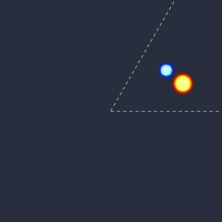
aaaa aaaa

(a) Phantom $f(x)$

aaaa

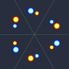
(b) Corresponding $f_{O}(x)$, $N=3$

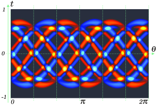
(c) Projections $\left(\mathcal{R}f_{O}\right)(t,\omega(\theta))$

aa

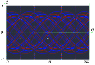
(d) Error in the reconstructed projections

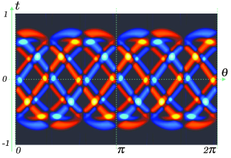
(e) Reconstruction from $p(t,y)$ with $|y|\leq 300$

a

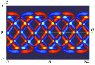
(f) Reconstruction from noisy data, $|y|\leq 300$

Figure 3: Example of reconstructing projections from $p(t,y)$ in 2D, $N=3$

5 Numerical simulations

In this section our formulas for reconstructing Radon projections are tested in two numerical simulations, one in 2D and the other one in 3D. The goal of these numerical experiments is to illustrate the exactness of the formulas, rather than to model realistic thermo- or photo- acoustic reconstruction. To this end, we did not simulate measurement noise, and did not study the effects of truncation of the acquisition surfaces. Moreover, when modeling the forward problem, an effort was made to sample solution of the wave equation on a grid covering the whole infinite boundary $\partial Q$. Clearly, this cannot be done numerically on a uniform grid. We, thus, used grids that are uniform on parts of the boundary relatively close to the origin (e.g. $|y|$ is less than several hundreds), and that are getting progressively coarser for larger values of $|y|.$

As stated by Corollary 15, for a particular direction of $\omega$ integration is done only over a finite subset of $\partial Q.$ The remote parts of $\partial Q$ are only needed for computing projections with $\omega$ near parallel to one of the parts of the boundary. Since remote parts of $\partial Q$ were sampled very coarsely, values of reconstructed projections corresponding to such directions of $\omega$ were less accurate.

5.1 A corner-like domain in 2D

Consider a problem of reconstructing Radon projections from solution of the wave equation known on $\partial Q$ consisting of two rays with angle $\beta=\pi/3$ between them.  This geometry corresponds to a subset of Coxeter cross with $N$ equal to $3.$ As a phantom $f(x)$, we use a linear combination $f(x)=h_{1}(x)-h_{2}(x)$ of functions $h_{j},$ $j=1,2,$ in the form

$$h_{j}=h\left(\frac{|x-x_{j}|}{r_{j}}\right),$$ (38)

where $h(s)$ is a smooth function with a maximum equal to 1, at $s=0$, and vanishing with several of its derivatives at $s=1.$ This phantom is plotted in figure 3(a). The odd part $f_{O}(x)$ of the function $f(x)$ is defined by formula (6); it is shown in figure 3(b).

Values of $p(t,y)$ corresponding to the chosen phantom $f(x)$ were computed on $\partial Q$ by first computing circular averages $M(y,r)$ defined by the equation

$$M(y,r)\equiv\int\limits_{\mathbb{S}^{1}}\frac{f(y+r\alpha)}{\sqrt{t^{2}-|r|^{2}}}d\alpha,$$

and by exploiting a well known connection between $p(t,y)$ and $M(y,r):$

$$p(t,y) =\frac{\partial}{\partial t}\int\limits_{\Omega}f(x)G^{+}(t,y-x)dx=\frac{\partial}{\partial t}\int\limits_{\Omega}f(y+z)G^{+}(t,z)dz$$

$$=\frac{1}{2\pi}\frac{\partial}{\partial t}\int\limits_{t}^{\infty}\int\limits_{\mathbb{S}^{1}}\frac{f(y+r\alpha)}{\sqrt{t^{2}-|r|^{2}}}d\alpha\ rdr=\frac{1}{2\pi}\frac{\partial}{\partial t}\int\limits_{t}^{\infty}\frac{M(y,r)}{\sqrt{t^{2}-|r|^{2}}}\ rdr.$$

The Abel transform of $M(y,r)$ and its time derivative were computed numerically.

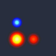
(a) Phantom, $z=0.3$

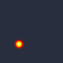
(b) Phantom, $z=0.6$

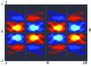
(c) Projections $\left(\mathcal{R}f_{O}\right)(t,\omega(\theta,\varphi_{0}))$

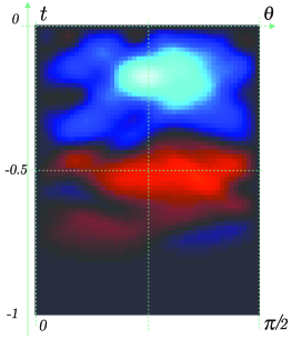
aaa aaa

(d) Projections on $(-1,0)\times(0,\pi/2)$, $\varphi=\varphi_{0}$

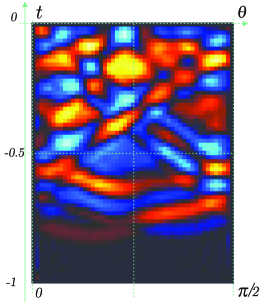
aa aaaa

(e) Recon. error on $(-1,0)\times(0,\pi/2)$, $\varphi=\varphi_{0}$

Figure 4: Reconstructing projections $\left(\mathcal{R}f_{O}\right)(t,\omega(\theta,\varphi))$ from values of $p(t,y)$ known on $\partial Q$ in 3D

For further comparison, the Radon projections $\left(\mathcal{R}\left[f_{O}\right]\right)(t,\omega(\theta))$ of $f_{O}(x)$ were computed first using the exact $f_{O}(x).$The result is shown in figure 3(c). One can clearly see in this figure symmetries described by equations (34)-(36). Next, we reconstructed the values of projections from $p(t,y)$ using formulas (32)-(36). On a gray scale (or color) plot the result is indistinguishable from the one in figure 3(c).  The plot of the difference between the reconstructed and known projections is shown in figure 3(d). One can notice that the error for values of $\theta$ close to $\frac{\pi k}{3},$ $k\in\mathbb{Z}$, is larger than for the rest of these values. An explanation was presented right before the start of this section. In an $L_{\infty}$-norm, the relative error over the whole range of values $t$ and $\theta$ is about 3%. If values of $\theta$ close to $\frac{\pi k}{3}$ are excluded from the comparison, this error drops to about 1%. At least a part of this error is due to the error in computing $p(t,y)$ by a three-step process involving finding circular averages, computing the Abel transform, and subsequent numerical differentiation.

In figure 3(e) we present an image reconstructed from data $p(t,y)$ known only for values $|y|\leq 300$. According to Theorem 17 applied with values $r_{0}=1$, $R=300$, our formulas yield exact reconstruction only for values of $\omega(\gamma)$ with $\gamma\in\bigcup\limits_{k=0}^{5}[6.62^{\circ}+k60^{\circ},(k+1)60^{\circ}-6.62^{\circ}]$. If one examines the image in part (e) only within this set of values, the error is similar to that shown in figure 3(d). For other values of $\gamma$ the error is larger, and can be noticed in a high-resolution version of the figure.

Figure 3(f) demonstrates reconstruction from noisy (and truncated in $y$) data. A $100\%$ noise (in $L_{2}$ norm) was added to values $p(t,y)$ at each point $y$ with $|y|\leq 300$, on the time intervals of length 2 starting at the time of arrival of the acoustic waves to point $y$. The effect of noise is noticeable in the figure; the relative $L_{\infty}$ norm of the error is about $25\%$. This error, however, is quite small taking into account the high level of noise in the data — as one would expect in view of the highly stable nature of our reconstruction formulas.

5.2 Boundary of an octet in 3D

In the second numerical experiment we reconstructed Radon projections of a function from solution of the wave equation known on a boundary $\partial Q$ of the first octet in 3D. As a phantom $f(x)$ defined within the intersection of the unit ball and the first octet, we used a linear combination of four functions in the form (38). The centers $x_{j}$ of these functions lied either in the plane $z=0.3$ or plane $z=0.6.$ The cross-sections of the phantom by these two planes are shown in figure 4, parts (a) and (b). Projections $\left(\mathcal{R}\left[f_{O}\right]\right)(t,\omega)$ of function $f_{O}(x)$ with $\omega$ parametrized in spherical coordinates (i.e., $\omega=(\sin\varphi\cos\theta,\sin\varphi\sin\theta,\cos\varphi))$ are shown in figure 4(c) for a fixed value of $\varphi=\varphi_{0}\thickapprox 53^{\circ}$. Symmetries expressed by equations (34) and (37) can be clearly seen in this figure. A magnified image of projections restricted to the region $(t,\theta)\in[-1,0]\times[0,\pi/2]$ with $\varphi=\varphi_{0}$ is shown in figure 4(d).

Modeling the forward problem (i.e., computing values of $p(t,y)$ on $\partial Q)$ is actually simpler in 3D than in 2D. For radial functions in the form (38) there exists an explicit exact formula [13] yielding values of $p(t,y).$ We precomputed these values on polar grids defined on each of three infinite faces constituting $\partial Q.$ The discretization step in the radial direction was uniform for relatively small values of the radius but became increasingly coarser for larger values.

Numerical reconstruction of projections from $p(t,y)$ performed using formulas (32), (34) and (37) in the region $(t,\theta)\in[-1,0]\times[0,\pi/2]$ yields data that are very close to the exact ones for most values of $\varphi.$ The results obtained for $\varphi=\varphi_{0}$ are indistinguishable from the exact values on a gray-scale or color plot. The error for $\varphi=\varphi_{0}$ is plotted in figure 4(e); the relative error in $L_{\infty}$ norm is about 0.1%. Similar error is observed for wide range of values of $\varphi$ except those close to $0$ or $\pi/2$. We explain a better accuracy obtained in 3D simulation by a better accuracy in modeling $p(t,y)$: in the 3D case these values are given by a theoretically exact formula.

6 Concluding remarks and acknowledgement

We presented explicit formulas that reconstruct Radon projections of $f_{O}$ from the values of the wave equation known on a boundary of an angular domain with $\pi/N$, $N=2,3,4,..$ (in 2D) or on the boundary of octet $Q$ (in 3D). Here are some additional thoughts:

• Since the solution of the wave equation in the case of constant speed of sound can be expressed through the spherical/circular means (and vice versa), finding Radon projections from these means is straightforward.

• Explicit relations between the Radon transform and the spherical/circular means were found in [4] in the case when the measurement surface is a hyperplane. The present results may be considered a generalization of that work, although the case of a hyperplane in 2D or 3D is not presented in our paper.

• General approach of this paper, as well as that of [4], is somewhat similar to the approach of Popov and Sushko [36, 37] who proposed a formula for finding Radon projections of a function from optoacoustic measurements. Their formula, however, yields a parametrix of the problem rather than the exact solution.

• Theorem 16 can be easily generalized to the case when the acquisition surface (in 3D) is the boundary of an infinite region bounded by three planes, with two of these planes intersecting at the angle $\pi/N$, $N=3,4,5...$ and the third plane perpendicular to the first two.

Acknowledgement: The author’s research is partially supported by the NSF, award NSF/DMS-1211521.

References

- [1] Andersson L-E 1988 On the determination of a function from spherical averages. SIAM J. Math. Anal. 19(1) 214–32
- [2] Agranovsky M and Quinto E T 1996 Injectivity of the spherical mean operator and related problems, in Complex analysis, harmonic analysis and applications (Deville R et al, eds), Addison Wesley Longman, London, 12–36
- [3] Beard P C 2011 Biomedical Photoacoustic Imaging Interface Focus 1(4) 602–31
- [4] Beltukov A and Feldman D 2009 Identities among Euclidean Sonar and Radon transforms Advances in Appl Math 42 23–41
- [5] Burgholzer P, Matt G J, Haltmeier M, and. Paltauf G 2007 Exact and approximative imaging methods for photoacoustic tomography using an arbitrary detection surface Phys Review E 75 046706
- [6] Cox B T, Arridge S R and Beard P C 2007 Photoacoustic tomography with a limited-aperture planar sensor and a reverberant cavity Inverse Problems 23(6) S95–S112
- [7] Denisjuk, A. 1999 Integral geometry on the family of semi-spheres. Fract. Calc. Appl. Anal. 2(1) 31–46
- [8] Ellwood R, Zhang E Z, Beard P C and Cox B T 2014 Photoacoustic imaging using acoustic reflectors to enhance planar arrays, submitted
- [9] Fawcett, J. A. 1985 Inversion of -dimensional spherical averages. SIAM J. Appl. Math. 45(2) 336–41
- [10] Finch D, Haltmeier M and Rakesh 2007 Inversion of spherical means and the wave equation in even dimensions SIAM J. Appl. Math. 68(2) 392–412
- [11] Finch D, Patch S K, and Rakesh 2004 Determining a function from its mean values over a family of spheres SIAM J. Math. Anal. 35(5) 1213–40
- [12] Fulks W and Guenther R B 1972 Hyperbolic Potential Theory Arch. Rational Mech. Anal. 49 79–88
- [13] Haltmeier M, Scherzer O, Burgholzer P, Nustero R and Paltauf G 2007 Thermoacoustic tomography and the circular Radon transform: Exact inversion formula Mathematical models & methods in applied sciences 17(4) 635–55
- [14] Haltmeier M 2013 Inversion of circular means and the wave equation on convex planar domains Computers & mathematics with applications 65(7) 1025–36
- [15] Holman B and Kunyansky L 2014 Gradual time reversal in thermo- and photo- acoustic tomography within a resonant cavity. Preprint
- [16] Kruger R A, Liu P, Fang Y R and Appledorn C R 1995 Photoacoustic ultrasound (PAUS) reconstruction tomography Med. Phys. 22 1605–09
- [17] Kruger R A, Reinecke D R, and Kruger G A 1999 Thermoacoustic computed tomography - technical considerations Med. Phys. 26 1832–7
- [18] Kruger R, KiserW, Reinecke D, and Kruger G (2003) Thermoacoustic computed tomography using a convential linear transducer array Med. Phys 30(5) 856–60
- [19] Kuchment P 2014 The Radon transform and medical imaging (Regional Conference Series in Applied Mathematics) CBMS - NSF
- [20] Kunyansky L, Holman B and Cox B T 2013 Photoacoustic tomography in a rectangular reflecting cavity Inverse Problems 29 125010
- [21] Kunyansky L 2007 Explicit inversion formulae for the spherical mean Radon transform Inverse problems 23 737–83
- [22] Kunyansky L 2007 A series solution and a fast algorithm for the inversion of the spherical mean Radon transform Inverse Problems, 23 (2007) S11–S20
- [23] Kunyansky L 2011 Reconstruction of a function from its spherical (circular) means with the centers lying on the surface of certain polygons and polyhedra Inverse Problems 27 025012
- [24] Kunyansky L 2012 Fast reconstruction algorithms for the thermoacoustic tomography in certain domains with cylindrical or spherical symmetries Inverse Problems and Imaging 6(1) 111–31
- [25] Li G, Xia J, Wang K, Maslov K, Anastasio MA, and Wang LV Tripling the detection view of high-frequency linear-array-based photoacoustic computed tomography by using two planar acoustic reflectors 2014 Quant Imaging Med Surg Oct 19. doi: 10.3978
- [26] Ma S, Yang S, and Guo H 2009 Limited-view photoacoustic imaging based on linear-array detection and filtered meanbackprojection- iterative reconstruction J. Applied Phys. 106 123104
- [27] F. Natterer 1986 The mathematics of computerized tomography, New York, Wiley
- [28] Natterer F 2012 Photo-acoustic inversion in convex domains Inverse Problems Imaging 6 315–20
- [29] M. Haltmeier M and Pereverzyev Jr. S 2014 The universal back-projection formula for spherical means and the wave equation on certain quadric hypersurfaces Preprint
- [30] Haltmeier M and Pereverzyev Jr. S 2014 Recovering a function from circular means or wave data on the boundary of parabolic domains Preprint
- [31] Norton S J 1980 Reconstruction of a two-dimensional reflecting medium over a circular domain: exact solution J. Acoust. Soc. Am. 67 1266–73
- [32] Norton S J and Linzer M 1981 Ultrasonic reflectivity imaging in three dimensions: exact inverse scattering solutions for plane, cylindrical, and spherical apertures IEEE Tran. Biomed. Eng. 28 200–2
- [33] Nguyen L V 2009 A family of inversion formulas in thermoacoustic tomography Inverse Problems and Imaging 3(4) 649–75
- [34] Oraevsky A A, Jacques S L, Esenaliev R O and Tittel F K 1994 Laser-based optoacoustic imaging in biological tissues Proc. SPIE 2134A 122–8
- [35] Palamodov V P 2012 A uniform reconstruction formula in integral geometry Inverse Problems 28 065014
- [36] Popov D A and Sushko D V 2002 A parametrix for the problem of optical-acoustic tomography Doklady Mathematics 65(1) 19–21
- [37] Popov D A and Sushko D V 2004 Image restoration in optical-acoustic tomography Problems of Information Transmission 40(3) 254–78
- [38] Salman Y 2014 An inversion formula for the spherical mean transform with data on an ellipsoid in two and three dimensions J. Math. Anal. Appl. 420 612–20
- [39] Ha-Duong T 2003 On Retarded Potential Boundary Integral Equations and their Discretization, in M. Ainsworth et al (Editors) Topics in computational wave propagation: direct and inverse problems, Lecture Notes in Computational Science and Engineering, 31. Springer-Verlag, Berlin, 301–36
- [40] Vladimirov V S 1971 Equations of mathematical physics. (Translated from the Russian by Audrey Littlewood. Edited by Alan Jeffrey.) Pure and Applied Mathematics, 3 Marcel Dekker, New York
- [41] Wang L V (Editor) 2009 Photoacoustic imaging and spectroscopy CRC Press
- [42] Xu M and Wang L V 2005 Universal back-projection algorithm for photoacoustic computed tomography Phys. Rev. E 71 016706