Analytical Derivation of Three Dimensional Vorticity Function for wave breaking in Surf Zone

I abstract

In this report, Mathematical model for generalized nonlinear three dimensional wave breaking equations was developed analytically using fully nonlinear extended Boussinesq equations to encompass rotational dynamics in wave breaking zone. The three dimensional equations for vorticity distributions are developed from Reynold based stress equations. Vorticity transport equations are also developed for wave breaking zone. This equations are basic model tools for numerical simulation of surf zone to explain wave breaking phenomena. The model reproduces most of the dynamics in the surf zone. Non linearity for wave height predictions is also shown close to the breaking both in shoaling as well as surf zone.

Keyword Wave breaking, Boussinesq equation, shallow water, surf zone. PACS : 47.32-y.

II Introduction

Wave breaking is one of the most complex phenomena that occurs in the near shore region. During propagation of wave from deep to shallow water, the wave field is transformed due to shoaling. Close to the shoreline, they become unstable and break. In the process of breaking, energy is redistributed from fairly organized wave motion to small scale turbulence, large scale currents and waves.
Classical Boussinesq theory provides a set of evolution equations for sueface water waves in the combined limit of weak nonlinearity (characterized by $\delta\leq 1$) and weak dispersion ($\mu\leq 1$) with the raio $\cfrac{\delta}{\mu^{\rm 2}}=O(1)$. the parameters represent a wave height to water deth ratio and a water depth to wavelength ratio, respectively.
It has been shown by numerous researchers that Boussinesq-type equations for varying water depth can describe nonlinear transformation in the shoaling region quite well. In the last couple of decades, a lot of research effort has gone into improving the predictive capability of these equations in the intermediate water-depth and close to the surf zone (see e.g. Nwogu nwogu , Madsen madsen , Wei wei ). It was established that to extend the validity of these equations to the deep water, higher order dispersive terms will have to be retained. To improve the predictive capability close to wave breaking, the higher order nonlinear terms are very important to include in the equation. However, all these models use additional terms that is artificially added to the momentum equation, which would then reproduce the main characteristic of a breaking wave, i.e. the reduction in wave height to describe wave breaking phenomena. Wave breaking in the software FUNWAVE (FUNWAVE is based on the model described by Nwogu nwogu ) is modeled by introducing momentum mixing term developed by Kennedy et al kennedy .
Starting with the works of Nwogu nwogu and Madsen madsen , most progress have been done to explain wave breaking phenomena. Shen shen addresses the problem with partially rotational flow. Vorticity dynamics and formation into the fluid is very important in the wave breaking as well surf zone. To address this problem, Veeramony & Svendsen veeramony2 derived breaking terms in Boussinesq equation assuming flow as a two-dimensional rotational flow. Here, the breaking process is modeled by assuming that vorticity is generated in the roller region of the breaking wave and solving vorticity transport equation to determine the distribution of the vorticity. This naturally introduces additional terms in the momentum equation which causes wave height reduction as well as changes in the velocity field. However, since this model is based on stream function formulation, it cannot be trivially extended to three-dimensional flow. The phenomena of wave breaking in Boussinesq equations are being modeled using quite few techniques which can preserve the wave shape as well as include energy dissipation mechanism. Shen shen developed a generalized form of Bousinesq equation in three dimensional by introducing vertical flow field with arbitrary vorticity distribution up to O($\mu^{\rm 2})$. But he did not describe momentum transport equation with full description of rotational flow. Recently, Zou et al zou addressed the problem by including the higher order terms in Boussinesq equation for two dimensinal flow. This model solves vorticity distribution based on the parametric form taken form surface roller experimental data. In this paper, we developed a general analytic form for breaking term for fully nonlinear set of Boussinesq equations for three dimensional vertical flow field near surf zone region. Derivation of breaking term from Reynold stress based vorticity transport equation was also developed to describe rotational field as a complete model for thorough understanding of wave breaking phenomena.
The term nonlinear indicates that no truncation based on powers of $\delta$ is employed. The paper is organized as follows: Section 2 discusses the basic governing equations for continuity and momentum with boundary conditions. Section 3 describes the equation for horizontal and vertical velocity distribution for potential and rotational components. In section 4, the breaking term is derived for velocity transport equation for fully nonlinear case and solved analytic form vorticity transport equation from Fourier series expansion. Reynold stresses are analyzed in the breaking region. In last section, results were discussed with conclusion. A parametric analysis of the role eddy viscosity profile is being discussed in detail.

III Basic Equations

We consider a three-dimensional wave field with free surface $\eta(x,y,t)$ propagating over a variable water depth $h(x,y)$. As we are primarily concerned with wave breaking, we only consider here wave propagation in shallow water. Wave in this region can be characterized by two non-dimensional parameters $\delta={a}/{h}$ and $\mu={h}/{l}$ where $a$ is the characteristic wave amplitude and $l$ the characteristic wave length. The parameter $\mu$ is a measure of frequency dispersion and $\delta$ that of the non linearity of the wave. In this study, since we are only considering shallow water waves, we only have to consider weakly dispersive waves (up to $O(\mu^{2})$) but have to retain all nonlinear terms. In this paper, the variables are non-dimensionalized using following scaling:

$$\begin{split}x=\hat{x}/l,y=\hat{y}/l,z=\hat{z}/h,\;t=\hat{t}\sqrt{gh}/l,\\ \hat{u}=\left(\delta\sqrt{gh}\right)u,\hat{v}=\left(\delta\sqrt{gh}\right)v,\hat{w}=\left(\delta\mu\sqrt{gh}\right)w\end{split}$$ (1)

where the $\;\hat{}\;$ represents the dimensional variables, $g$ is the acceleration due to gravity, $u$ and $v$ are the horizontal components of the velocity in the $x$ and $y$ directions respectively, $w$ is the vertical velocity. We start with the Eulerian equations of continuity and momentum in nondimensionalized form for velocity field ${\bf u}=(u,v,w)$ as:

$$\begin{split}\cfrac{\partial u}{\partial t}+{\delta}u\cfrac{\partial u}{\partial x}+{\delta}v\cfrac{\partial u}{\partial y}+{\delta}w\cfrac{\partial u}{\partial z}+\cfrac{\partial p}{\partial x}=0\\ \cfrac{\partial v}{\partial t}+{\delta}v\cfrac{\partial v}{\partial x}+{\delta}v\cfrac{\partial v}{\partial y}+{\delta}w\cfrac{\partial v}{\partial z}+\cfrac{\partial p}{\partial y}=0\\ {\delta\mu^{2}}\cfrac{\partial w}{\partial t}+{\delta^{2}\mu^{2}}u\cfrac{\partial w}{\partial x}+{\delta^{2}\mu^{2}}v\cfrac{\partial w}{\partial y}+{\delta^{2}\mu^{2}}w\cfrac{\partial w}{\partial z}+{\delta}\cfrac{\partial p}{\partial z}+1=0\end{split}$$ (2)

Since the fluid flow is rotational, we also have three dimensional vorticity field ${\bf s}=(s_{x},s_{y},s_{z})$ in the fluid defined as

$${\bf\bigtriangledown}\times{\bf u}={\bf s}$$ (3)

where $\bigtriangledown=(\partial/\partial x,\partial/\partial y,\partial/\partial z).$ The continuity equation then becomes,

$$\bigtriangledown\cdot u+\cfrac{\partial w}{\partial z}=0$$ (4)

Here $\bigtriangledown\cdot u=(\partial u/\partial x,\partial v/\partial y).$ The above equations satisfy two boundary conditions for velocity at bottom and at free surface. At the free surface ${\it z}=\eta(x,y,t)$, since particles are free to move with fluid velocity, the kinematic boundary condition is

$$w_{\rm\eta}={\bf u_{\rm\eta}}\cdot{\bf\bigtriangledown}\eta+\cfrac{\partial\eta}{\partial t}$$ (5)

and at bottom ${\it z=-h(x,y)}$

$$w_{b}=-u_{b}\cdot{\bigtriangledown}h$$ (6)

where ${\bf u_{\rm\eta}}=(u_{\rm\eta},v_{\rm\eta})$ is two component horizontal surface velocity. $\bigtriangledown\eta=(\eta_{\rm x},\eta_{\rm y}),$ $\bigtriangledown h=(h_{\rm x},h_{\rm y})$ refer to horizontal derivative with respect to x and y in all subsequent calculations. The horizontal component for vorticity field $\bf s=(s_{\rm y},-s_{\rm x})$ can be described as,

$$\cfrac{\partial u}{\partial z}-\mu^{\rm 2}{\bigtriangledown}w={\bf s}$$ (7)

with ${\bf u}=(u,v)$ as two component horizontal field whereas vertical component of vorticity expressed as

$$-s_{\rm z}=\cfrac{\partial u}{\partial y}-\cfrac{\partial v}{\partial x}$$ (8)

This is straightforward calculation from equation (6) and (8) which is the beginning equation in three dimensional vorticity field formulation.

$$\mu^{2}{\bigtriangledown}^{2}w+\frac{\partial^{2}w}{\partial z^{2}}=-{\bigtriangledown}\cdot s=S_{w}$$ (9)

$w$ represents the vertical velocity of the flow. In the above equation, once $w$ solved, horizontal component of velocity $u,v$ can be solved from vorticity relation. In weakly hydro static case ( $0<\mu^{2}\ll 1$ ), solution is typically obtained from iterative perturbation procedure with successive correction term up to $\mu^{2}$.

In case of breaking waves where vorticity is very strong, so $({\partial u}/{\partial z}\sim O(1)).$ We assume solution as, $u=u_{\rm o}+\mu^{\rm 2}u_{\rm 1}+O(\mu^{\rm 4})$ and $w=w_{\rm 0}+\mu^{\rm 2}w_{\rm 1}+O(\mu^{\rm 4})$ for horizontal and vertical velocity component. Under this assumption, Poisson equation becomes

$$\cfrac{\partial^{\rm 2}w_{\rm 0}}{\partial z^{\rm 2}}=S_{\rm w}$$ (10)

$$\cfrac{\partial^{\rm 2}w_{\rm 1}}{\partial z^{\rm 2}}=-\left[\cfrac{\partial^{\rm 2}w_{\rm 0}}{\partial x^{\rm 2}}+\cfrac{\partial^{\rm 2}w_{\rm 0}}{\partial y^{\rm 2}}\right]$$ (11)

$w_{0}$, $w_{1}$ can be calculated from bottom boundary conditions using equation (7) separately where the boundary conditions are,

$$\begin{split}w_{\rm{b0}}=-u_{\rm{b0}}\cdot{\bigtriangledown}h\\ w_{\rm{b1}}+u_{\rm{b1}}\cdot{\bigtriangledown}h=0\end{split}$$ (12)

at bottom boundary z = -h .
Since at any other depth ${\bf z}=z_{\rm r}$, w is constrained by continuity equation only, so the equation follows

$$\cfrac{\partial w}{\partial z}{]_{z}}_{r}=-{\bf\bigtriangledown}\cdot u_{\rm m}{]_{\rm z}}_{r}+\cfrac{\partial u}{\partial z}\cdot{\bf\bigtriangledown}z_{\rm r}{]_{\rm z}}_{r}$$ (13)

where $u_{\rm m}$ is velocity at any arbitrary depth $z_{r}$ . In Boussinesq equation, one may take depth average or any intermediate velocity for horizontal velocity between bottom and free surface as reference velocity. In the wave breaking zone where the vorticity is developed non uniformly, the equations become simpler with the choice of depth average velocity which includes contribution from surface vorticity gradient. We assume solution for velocity comes also from rotational contribution due to vorticity at the wave surface. So the velocity has both potential as well as rotational component, $u=u_{\rm p}+u_{\rm r}$ , $w=w_{\rm p}+w_{\rm r}$
We solve $w_{\rm 0},w_{\rm 1}$ and $u_{\rm 0},u_{\rm 1}$ at any depth $z_{\rm r}$

$$\frac{\partial w_{0}}{\partial z}{]_{z}}_{r}=-{\bf\bigtriangledown}\cdot(u_{m}-z_{r}s{]_{z}}_{r})+z_{r}{\bf\bigtriangledown}\cdot s$$ (14)

$$[\frac{\partial w_{1}}{\partial z}{]_{z}}_{r}=[{\bf\bigtriangledown}w_{0}{]_{z}}_{r}\cdot{\bf\bigtriangledown}z_{r}$$ (15)

$$\begin{split}\cfrac{\partial u_{0}}{\partial z}=s\cfrac{\partial u_{1}}{\partial z}={\bigtriangledown}w_{0}\end{split}$$ (16)

with boundary condition $[u_{\rm 0}{]_{\rm z}}_{\rm r}=u_{\rm r}$ and $[u_{\rm 1}{]_{\rm z}}_{\rm r}=0$
Equations (4) - (16) form basic shallow water Boussinesq equations.

IV Equation for horizontal velocity

In the surf zone, vorticity grows very strongly as a non uniform function over depth. Following Shen [2000], we define reference velocity as $\tilde{u}=\bar{u}+\bigtriangleup\bar{u}-\eta s_{\rm\eta}$ in terms of depth average velocity ${\it\bar{u}}$ and magnitude of vorticity at free surface $s_{\rm\eta}$ with the assumption of $\bigtriangledown\cdot s\neq 0$. we set here $z_{\rm r}=\eta$ as linear calibration for $z_{\rm r}=r(\eta+h)-h$ does not hold here in presence of nonuniform velocity as wave dispersion properties change both spatially and temporally with vorticity. And boundary condition can be set as

$$\cfrac{\partial w}{\partial z}|_{\rm\eta}={\bf\bigtriangledown}\cdot\tilde{u}+\eta({\bf\bigtriangledown}\cdot s_{\rm\eta})$$ (17)

Integrating equation (9) from bottom to surface and applying boundary condition to (16) we get $w_{0}$ as ,

$$w_{\rm 0}=w_{\rm{b0}}-(-{\bf\bigtriangledown}\cdot\tilde{u}+\eta{\bf\bigtriangledown}\cdot s_{\rm{\eta}})H_{\rm z}-S_{\rm{w0}}$$ (18)

where

$$S_{\rm{w0}}=\int\int(-\bigtriangledown\cdot s)dzdz$$

is the vertical velocity distribution generated by horizontal divergence of vorticity added to surface velocity. Now, once $w_{\rm 0}$ is calculated, $u_{\rm 1}$ can be calculated from eqn (15) with surface boundary condition $\{{u_{\rm 0}\}}_{\rm\eta}=u_{\rm m}$ and $\{u_{\rm 1}\}_{\rm\eta}=0$ Finally, we calculate horizontal velocity as

$$\begin{split}u(z)=u_{\rm\eta}-\int_{\rm z}^{\rm\eta}sdz+{\mu}^{\rm 2}(S_{\rm{wl}}-\bar{S}_{\rm{wl}})\\ +\cfrac{\mu^{\rm 2}}{2}({H_{\rm\eta}^{\rm 2}}-{H_{\rm z}}^{\rm 2}){\bigtriangledown}(\bigtriangledown\cdot\tilde{u}-{\eta}{\bigtriangledown}\cdot s_{\rm\eta})\\ +{\mu}^{\rm 2}(H_{\rm\eta}-H_{\rm z})\left[{\bf\bigtriangledown}((\tilde{u}+\eta s_{\rm\eta})\cdot{\bf\bigtriangledown}h)+({\bf\bigtriangledown}\cdot\tilde{u}-\eta\bigtriangledown\cdot s_{\rm\eta})\bigtriangledown h\right]+O(\mu^{\rm 4})\end{split}$$ (19)

which on averaging over depth yields,

$$\begin{split}\bar{u}=u_{\rm\eta}-\bigtriangleup\bar{u}+\cfrac{\mu^{\rm 2}}{3}{H_{\rm\eta}}^{\rm 2}\bigtriangledown\left[\bigtriangledown\cdot\tilde{u}-{\eta}{\bigtriangledown}\cdot s_{\rm\eta}\right]-\cfrac{\mu^{\rm 2}}{2}H_{\rm\eta}[{\bigtriangledown}\tilde{u}+{\eta}s_{\rm\eta}]\cdot{\bigtriangledown}h\\ -({\bigtriangledown}\cdot\tilde{u}-{\eta}{\bigtriangledown}\cdot s_{\rm\eta}){\bigtriangledown}h+O(\mu^{\rm 4})\end{split}$$ (20)

$\bigtriangleup\bar{u}=\cfrac{1}{H_{\eta}}{\int}_{\rm{-h}}^{\rm\eta}\bigtriangleup u(z)dz$ is the average surface velocity contribution due to vorticity and it is significant for suspended sediment particles in the flow. The term $\bigtriangleup{\bf u(z)}=\int_{\rm z}^{\eta}sdz$ is the change due to depth variation of vorticity ${\bf s}$. The total water depth $H_{\rm z}$ and surface elevation $H_{\eta}$ are taken as $H_{\rm z}$ = z + h and $H_{\rm\eta}=\eta+h$. The contribution for velocity has and rotational component apart from potential due to vorticity generation.
After we redefine $H_{\rm\eta}=d$ and $z={H_{z}}/{H_{\rm\eta}}$, we express potential and rotational component up to order $O(\mu^{\rm 2})$ as,

$$\begin{split}u_{p}(z)=\bar{u}_{p}+\cfrac{\mu^{2}}{2}(\cfrac{1}{3}-z^{2}){d^{2}}\bigtriangledown(\bigtriangledown\cdot\bar{u}_{p})\\ +{\mu^{2}}(\cfrac{1}{2}-z)d\left[\bigtriangledown(\tilde{u}_{p}\cdot\bigtriangledown h)+(\bigtriangledown\cdot\tilde{u}_{p})\bigtriangledown h\right]\\ u_{r}(z)=\tilde{u}_{r}-\bigtriangleup u(z)+\eta s_{\eta}+\mu^{2}(S_{{wl}}-\bar{S}_{{wl}})\\ -\cfrac{\mu^{2}}{2}(\frac{1}{3}-z^{2})d^{2}{\eta}\bigtriangledown(\bigtriangledown\cdot s_{\eta})\\ -{\mu^{2}}(\cfrac{1}{2}-z)d{\eta}\left[(\bigtriangledown\cdot s_{\eta})\bigtriangledown h-\bigtriangledown(s_{\eta}\cdot\bigtriangledown h)\right]\end{split}$$ (21)

Similar expressions for vertical velocity are

$$\begin{split}w_{p}(z)=-(h+z)\bigtriangledown\cdot u_{\rm p}(z)\\ =-\bigtriangledown\cdot\left[(h+z)\tilde{u}_{\rm p}\right]-\cfrac{\mu^{2}}{2}((\cfrac{1}{3}-z^{2})\bigtriangledown\cdot\left[d^{2}(h+z)(\bigtriangledown(\bigtriangledown\cdot\tilde{u}_{p})\right]\\ -\mu^{2}(\frac{1}{2}-z)\left[\bigtriangledown\cdot(h+z)(\bigtriangledown(u_{p}\cdot\bigtriangledown h)+(\bigtriangledown\cdot u_{p})\bigtriangledown h)\right]\end{split}$$ (22)

$$\begin{split}w_{r}(z)=-\bigtriangledown\cdot(h+z)\tilde{u}_{r}-\bigtriangledown\cdot\left[(h+z)\eta s_{\eta}\right]\\ -\cfrac{\mu^{2}}{2}\left[\bigtriangledown\cdot(h+z)(\cfrac{1}{3}-z^{2})d^{2}{\bigtriangledown}(\eta\bigtriangledown\cdot s_{\eta})\right]\\ +{\mu^{2}}\bigtriangledown\cdot[(\frac{1}{2}-z)d\left[\bigtriangledown(\eta s_{\eta}.\bigtriangledown h)-(\bigtriangledown\cdot\eta s_{\eta})\bigtriangledown h\right]\end{split}$$ (23)

V Breaking Model [Our case: fully nonlinear]

The most obvious approach to solve Boussinesq equation is to drop notion of pursuing an expansion in powers of $\delta$ and instead use weakly dispersive expression for $\phi$ or horizontal velocity in the form of power series in $\mu^{\rm 2}$ to evaluate complete surface boundary condition. We refer to this procedure as $\it{fullynonlinear}$ in the sense that all of the availble information on velocities is used to evaluate boundary conditions. Conventional time dependent Boussinesq equations for surface wave height and consequent breaking term calculation are very straight forward and have benn calculated in case of irrotational waves. Here we take up fully nonlinear calculation as vorticity becomes a large fraction of water depth in the surf zone or shoaling waves. While developing Boussinesq equations for horizontal momentum, we retain up to order O($\delta^{\rm 2})$ and O($\delta\mu^{2})$ in our fully nonlinear calculation. Fully nonlinear Boussinesq equations for long wave have been derived by Mei [1983] for flat bottom and by Wei et al wei for variable bottom surface in case of irrotational wave. Shen shen addressed problems in developing generalized three dimensional irrotational propagating wave field to include rotational motion in general but did not describe the vorticity breaking terms. For horizontal propagation of waves, the three dimensional problem can be reduced in terms of two horizontal velocity by integrating over depth and retaining up to order $O(\delta^{\rm 2})$ and $O(\delta\mu^{\rm 2})$ As horizontal velocity is governed by momentum equation at the surface $\eta$ by,

$$\cfrac{Du}{Dt}{|}_{\rm\eta}=(\cfrac{Dw}{Dt}{|}_{\rm\eta}+1){\bigtriangledown}\eta$$ (24)

In the surf zone region of sloping beach, waves break due to high vorticity and the breaking of wave later being converted to turbulence. So horizontal variation of water depth ${\it h(x,y)}$ must be considered in this case. We express surface propagation equation in terms of average velocity description and total time derivative of horizontal momentum can be written as,

$$\cfrac{D\bar{u}}{Dt}{|}_{\rm\eta}=\cfrac{\partial u}{\partial t}{|}_{\eta}+u_{\rm\eta}\cdot(\bigtriangledown u){|}_{\rm\eta}$$ (25)

where surface velocity is given by,

$$\begin{split}u_{\rm\eta}=\bar{u}+{\eta}s_{\rm\eta}-\cfrac{\mu^{\rm 2}}{3}d^{\rm 2}\bigtriangledown\left(\bigtriangledown\cdot\tilde{u}-{\eta}{\bigtriangledown}\cdot s_{\rm\eta}\right)+\cfrac{\mu^{\rm 2}}{2}d\{{\bigtriangledown}\left(\tilde{u}-{\Delta}\bar{u}{|}_{\rm{-h}}+{\eta}s_{\rm\eta}\right)\cdot{\bigtriangledown}h\}\\ \end{split}$$ (26)

We consider $\bigtriangledown H_{\eta}=\bigtriangledown\eta+\bigtriangledown h$ for wavy bottom

$$\begin{split}\cfrac{Du}{Dt}|_{\rm\eta}=\cfrac{\partial\tilde{u}}{\partial t}++\eta\cfrac{\partial s_{\rm\eta}}{\partial t}+\tilde{u}\cdot\bigtriangledown\tilde{u}\end{split}$$ (27)

$$\begin{split}\cfrac{Du}{Dt}|_{\rm\eta}=\cfrac{\partial\tilde{u}}{\partial t}++{\eta}\cfrac{\partial s_{\rm\eta}}{\partial t}+\tilde{u}\cdot\bigtriangledown\tilde{u}-\cfrac{\mu^{\rm 2}}{3}d^{\rm 2}\{{\bigtriangledown}(\bigtriangledown\cdot\cfrac{\partial\tilde{u}}{\partial t}-{\eta}{\bigtriangledown}\cdot\cfrac{\partial s_{\eta}}{\partial t})+\tilde{u}\cdot\bigtriangledown(\bigtriangledown\cdot{\tilde{u}}-{\eta}{\bigtriangledown}\cdot s_{\rm\eta})\\ +\cfrac{\mu^{\rm 2}}{2}d\{\bigtriangledown(\cfrac{\partial\tilde{u}}{\partial t}+{\eta}\cfrac{\partial s_{\rm\eta}}{\partial t})\cdot{\bigtriangledown}h\\ -(\bigtriangledown\cdot\cfrac{\partial\tilde{u}}{\partial t}-{\eta}\bigtriangledown\cdot\cfrac{\partial s_{\rm\eta}}{\partial t}){\bigtriangledown}h+\tilde{u}\cdot\bigtriangledown\}+O(\mu^{4})\end{split}$$ (28)

This long wave momentum equation upon simplification over flat bottom case can be compared to the one derived by Shen [2000] The vertical velocity can be obtained similarly,

$$\cfrac{Dw}{Dt}|_{\eta}=\cfrac{\partial w}{\partial t}|_{\rm\eta}+u_{\eta}\cdot\bigtriangledown w_{\eta}+w\cfrac{\partial w}{\partial z}|_{\rm\eta}$$ (29)

So, we can write the horizontal momentum equation as,

$$\begin{split}\cfrac{\partial\tilde{u}}{\partial t}+\tilde{u}\cdot\bigtriangledown\tilde{u}+\bigtriangledown\eta=\cfrac{\mu^{\rm 2}}{3}d^{\rm 2}\{\bigtriangledown(\bigtriangledown\cdot\tilde{u})\cdot\bigtriangledown\tilde{u}+\bigtriangledown(\bigtriangledown\cdot\cfrac{\partial\tilde{u}}{\partial t})\\ +(\tilde{u}\cdot\bigtriangledown(\bigtriangledown\cdot\tilde{u})\}-\mu^{\rm 2}d\{\bigtriangledown\cdot\frac{\partial\tilde{u}}{\partial t}-d^{\rm 2}\bigtriangledown(\bigtriangledown\cdot\cfrac{\partial\tilde{u}}{\partial t})+(\bigtriangledown\cdot u_{\eta})^{\rm 2}\\ -\tilde{u}\cdot\bigtriangledown(\bigtriangledown\cdot\tilde{u})\}\bigtriangledown{\eta}\end{split}$$ (30)

$\tilde{u}$ is defined in previous section. In contrast to the result by Shen shen , additional contribution factor here arises from vorticity variation which is significant for surf zone wave. Wei et al wei also calculated breaking term for irrotational long wave momentum equation over a variable bottom wave. The intermediate depth velocity $z_{\rm\alpha}$ is being used there proportional to h instead of depth average velocity used here which may not be valid inside the fluid. The use of $z_{\rm r}$ in our approach avoids this difficulty. Finally we try to generalize equation by solving vorticity from vorticity transport equation in next section.

VI Vorticity transport equation in breaking zone

Madsen and Svendsen madsen used a cubic vertical distribution of rotational velocity based on roller jump data which can not considered in three dimension case as it is not guaranteed to bring accuracy in the simulation. So we try to solve vorticity function from Reynold stress based equation.

$$\cfrac{\partial u}{\partial t}+(u\cdot\bigtriangledown)u=-\cfrac{1}{\rho}{\bigtriangledown p}$$ (31)

Taking the curl on both sides and use vorticity function $s=\bigtriangledown\times u$ we get,

$$\cfrac{\partial s}{\partial t}-(s\cdot\bigtriangledown)s+(u\cdot\bigtriangledown)s={\nu}{\bigtriangledown}^{\rm 2}s$$ (32)

$(s\cdot\bigtriangledown)s$ is called ”vorticity stretching” factor and is the gradient in vorticity value. This term leads to change of rotation of material particles present in the flow to the beach. Contribution of this term can not be incorporated from two dimension roller jump data.

We generalize the equation in three dimension as

$$\begin{split}\cfrac{\partial s}{\partial t}+{\delta u}\cfrac{\partial s}{\partial x}+{\delta v}\cfrac{\partial s}{\partial y}+{\delta w}\cfrac{\partial s}{\partial z}-{\delta s}\cfrac{\partial u}{\partial x}-{\delta s}\cfrac{\partial v}{\partial y}-{\delta s}\cfrac{\partial w}{\partial z}\\ =\nu\left[{\mu}^{\rm 2}\cfrac{\partial^{\rm 2}s}{{\partial x}^{\rm 2}}+{\mu}^{\rm 2}\cfrac{\partial^{\rm 2}s}{{\partial y}^{\rm 2}}+\cfrac{\partial^{\rm 2}s}{{\partial z}^{\rm 2}}\right]\end{split}$$ (33)

After changing the variable from (x,y,z,t) to wave following coordinates $(x,y,\sigma,t)$, we write the vorticity equation as

$$\begin{split}\cfrac{\partial s}{\partial t}-\cfrac{\delta\sigma}{(h+\delta\eta)}\cfrac{\partial\eta}{\partial t}\cfrac{\partial s}{\partial\sigma}+\delta u(\bigtriangledown\cdot s)-{\delta}s(\bigtriangledown\cdot u)-\cfrac{\delta}{(h+\delta\eta)}\left[s\cfrac{\partial w}{\partial\sigma}-w\cfrac{\partial s}{\partial\sigma}\right]\\ -{\delta}^{\rm 2}\frac{\sigma u}{(h+\delta\eta)}(\bigtriangledown\cdot\eta)\cfrac{\partial s}{\partial\sigma}+{\delta}^{\rm 2}\cfrac{\sigma s}{(h+\delta\eta)}(\bigtriangledown\cdot\eta)\cfrac{\partial u}{\partial\sigma}\\ =\nu\left[{\mu^{\rm 2}}\bigtriangledown^{\rm 2}s+\cfrac{1}{(h+\delta\eta)}\cfrac{\partial^{\rm 2}s}{\partial\sigma^{\rm 2}}\right]+O(\mu^{\rm 2})+O(h_{\rm x})+O(h_{\rm y})\end{split}$$ (34)

The boundary conditions in new coordinate system are,

$$\begin{split}s(\sigma=1,t)=s(x,y,t);\\ s(\sigma=0,t)=0;\\ s(\sigma,t=0)=0\end{split}$$ (35)

After we redefine $s=\Omega+\sigma{\omega}_{s}$, which transforms the equation,

$$\begin{split}\cfrac{\partial\Omega}{\partial t}+{\sigma}\frac{\partial\omega_{s}}{\partial t}-{\delta}\frac{\sigma}{(h+{\delta}{\eta})}\left[\sigma\frac{\partial\eta}{\partial t}-\cfrac{\partial\eta}{\partial t}\frac{\partial\Omega}{\partial\sigma}\right]\\ +{\delta}u(\bigtriangledown\cdot\Omega)-\cfrac{\delta\sigma}{(h+\delta\eta)}(\bigtriangledown\cdot\eta)\cfrac{\partial\Omega}{\partial\sigma}-\cfrac{\delta\sigma^{2}}{(h+\delta\eta)}(\bigtriangledown\cdot\eta)\\ +\cfrac{\delta u}{(h+\delta\eta)}\cfrac{\partial\Omega}{\partial\sigma}+\cfrac{\delta w}{(h+\delta\eta)}\omega_{s}\\ -\cfrac{\delta\Omega}{(h+\delta\eta)}\cfrac{\partial w}{\partial\sigma}-\cfrac{\delta\sigma\omega_{s}}{(h+\delta\eta)}\cfrac{\partial w}{\partial\sigma}\\ -\delta\Omega(\bigtriangledown\cdot u)-{\delta}{\sigma}\omega_{s}(\bigtriangledown\cdot u)+\cfrac{\delta^{2}\sigma\Omega}{(h+\delta\eta)}(\bigtriangledown\cdot\eta)\cfrac{\partial u}{\partial\sigma}+\cfrac{\delta^{2}\sigma\Omega}{(h+\delta\eta)}(\bigtriangledown\cdot\Omega)\cfrac{\partial u}{\partial\sigma}\\ +\frac{\delta^{2}\sigma\omega_{s}}{(h+\delta\eta)}(\bigtriangledown\cdot\eta)\cfrac{\partial u}{\partial\sigma}\end{split}$$ (36)

with new boundary,

$$\begin{split}\Omega(\sigma=1,t)=0\\ \Omega(\sigma=0,t)=0\end{split}$$ (37)

with initial condition $\Omega(\sigma,t=0)=0$. This additional equation can be solved numerically as done by Briganti et al. briganti for the two dimensional case or an analytical solution can be formulated as shown by Veeramony & Svendsen veeramony2 . The analytical solution can be calculated by assuming $\Omega=\omega^{\rm{(1)}}+{\delta}{\omega}^{\rm{(2)}}$ which gives first and second solution as O(1) Problem

$$\cfrac{\partial\omega^{\rm{(1)}}}{\partial t}+{\sigma}\cfrac{\partial\omega_{\rm s}}{\partial t}=\cfrac{\nu}{h^{\rm 2}}\cfrac{\partial^{\rm 2}\omega^{\rm{(1)}}}{\partial t^{\rm 2}}$$ (38)

where the solution is

$$F_{\rm n}^{\rm{(1)}}=(-1)^{\rm n}\cfrac{2}{n\pi}\cfrac{\partial{\omega}_{\rm s}}{\partial t}$$ (39)

assuming $-\sigma\cfrac{\partial{\omega}_{\rm s}}{\partial t}={\sum_{\rm n=1}}^{\infty}F_{\rm n}^{\rm 1}\sin(n\pi\sigma)$ And to solve $\omega^{\rm{(1)}}$, assume $\omega^{\rm{(1)}}=\Sigma_{\rm n}G_{\rm n}^{\rm{(1)}}sin(n\pi\sigma)$ which gives zeroth order solution as

$$G_{\rm n}^{\rm{(1)}}=(-1)^{\rm n}\cfrac{2}{n\pi}\int_{\rm 0}^{\rm t}\cfrac{\partial\omega_{\rm s}}{\partial\tau}e^{\rm{n^{\rm 2}}{\pi}^{\rm 2}{\kappa(\tau-t)}}d{\tau}$$ (40)

To consider O($\delta$)Problem

$$\cfrac{\partial\omega^{(2)}}{\partial\sigma}-\cfrac{\nu}{h}\cfrac{\partial^{2}\omega^{\rm(2)}}{\partial\sigma^{\rm 2}}=F^{\rm(2)}$$ (41)

where

$$\begin{split}F^{\rm{(2)}}=\cfrac{\sigma}{h}\cfrac{\partial\eta}{\partial t}\cfrac{\partial\omega^{(1)}}{\partial\sigma}-\cfrac{\sigma^{\rm 2}}{h}\cfrac{\partial\eta}{\partial t}-\cfrac{\sigma}{h}(\bigtriangledown\cdot\eta)\cfrac{\partial\omega^{\rm(1)}}{\partial\sigma}-\cfrac{\sigma^{\rm 2}}{h}(\bigtriangledown\cdot\eta)+u(\bigtriangledown\cdot\omega^{\rm(1)})\\ +\cfrac{u}{h}\cfrac{\partial\omega^{\rm(1)}}{\partial\sigma}\end{split}$$ (42)

To solve above equation, assume $\omega^{\rm(2)}=\Sigma_{n}^{{(2)}}sin(n\pi\sigma)$ where solution becomes

$$G_{\rm n}^{\rm{(2)}}=2\int_{0}^{\rm 1}F_{\rm n}^{\rm{(2)}}e^{n^{2}\pi^{\rm 2}\kappa(\tau-t)}d{\tau}$$ (43)

with

$$F_{\rm n}^{\rm{(2)}}=2{\int}_{\rm 0}^{\rm 1}F^{\rm(2)}sin(n{\pi}{\sigma})d{\sigma}$$ (44)

The solution for vorticity s becomes,

$$s={\sigma}{\omega}_{\rm s}+\Sigma_{\rm 1}{G_{\rm n}}^{\rm(1)}sin(n{\pi}{\sigma})+{\Sigma}_{\rm 1}{G_{\rm n}}^{\rm(2)}sin(n{\pi}{\sigma})$$ (45)

To solve breaking term, we need value of $\omega_{\rm s}$ for boundary and eddy viscosity value as input data. The parametric form of vertical profile of eddy viscosity is being applied to calculate vorticity function using various experimental data. The eddy viscosity distribution over the water column $N(z)$ is assumed such that its maximum value is located at the water surface except at the roller where the maximum is located at the lower edge of the roller. The value is estimated by a mixing length hypothesis and $\nu_{\rm t}$ is given by,

$$\nu_{\rm t}(z,x)=\nu_{\rm{0t}}h(x)\sqrt{gh(x)}N(z)$$ (46)

The best fit for $\omega_{\rm s}$ based on experimental data for hydraulic jump svendsen ,

$$\omega_{\rm s}=15.75(1-\cfrac{x-x_{\rm t}}{l_{\rm r}})(1-e^{\rm{-40\cfrac{x-x_{\rm t}}{l_{\rm r}}}})$$ (47)

where $x_{\rm t}$ is the position of the toe of the roller and $l_{\rm r}$ is the roller length. Figure 1. shows our analytical calculation time evolution of vorticity profile for $\nu_{\rm{t0}}=0.03$.

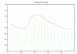
Figure 1: Figure 1. shows analytical calculation for time evolution of vorticity profile

VII Conclusion

Finally we conclude here by developing a most generalized form fully nonlinear Boussinesq equations for wave propagation in surf zone region with variable bathymetry. The vorticity distribution was calculated using Vorticity Transport Equation(VTE). In the wave breaking zone, vorticity generated by the shear stress of current is very strong, we showed in our calculation the contribution to the surface velocity due to vorticity variation which has significant contribution in fluid flow. These extra terms in generalized equation complicate the numerical technique as these terms are present in the equation in multiple form of equations for vorticity components which has to be solved in coupled solution technique. Veeramony veeramony1 used simplified formulation by taking constant eddy viscosity value but this oversimplified case may bring inaccuracy in calculation. Briganti et.al briganti formulated a numerical technique scheme to solve VTE using generalized depth variable eddy viscosity $\nu=\nu(x,y)$ in two dimension case. In three dimensional formulation, the nonlinear terms in the vorticity transport equation(VTE) will complicate the calculation and so proper numerical technique have to be developed. Turbulence develops because of the instability of vortical flow, turbulence injection can be explained from vortical function development.

VIII list of Symbols

$a$ – Wave Amplitude; $l$ – Characteristic wave length; ${\bf s}$ – Vorticity function; $g$ – gravitational Constant; $f$ – bottom friction constant

IX Acknowledgment

Finnaly we speacially R. Dutta thanks Office of Naval Research Lab (NRL) under grant [GR001820] for financial support of this work.

References

- (1) Briganti R. & Musumeci R.E.,(2004), Boussinesq Modeling of Breaking Waves: Description of Turbulence, J. Geophys. Research, 109, (2004), C07015.
- (2) Kennedy, A.B., Chen Q., Kirby J.T. & Dalrymple R.A., Boussinesq modeling of wave transformation, Breaking and run-up I: One dimension, J. Waterway, Port, Coastal & Ocean Engineering, 126,(1999), 206-214.
- (3) Madsen,P.A. & Svendsen I.A., Turbulent Bores and Hydraulic Jump, J.Fluid Mech, 129,(1983), 1-25.
- (4) Mei, C.C, The Applied Dynamics of Ocean Surface Waves, J. Wiley and sons,(1983), 740.
- (5) Nwogu, O., An alternative form of Boussinesq equations for near shore wave propagation, ASCE J.Waterway Port, Coastal and Ocean Engineering,119, (1993),618- 638.
- (6) Shen C., Constituent Boussinesq Equations for Waves and Currents, J. Physical Oceanography,31,(2000), 850-859.
- (7) Svendsen IB.A, Veeramony J, Bakunin J. & Kirby T., The Flow in Weak Turbulent Hydraulic Jumps, J. Fluid Mech,bf 418,(2000), 25-57.
- (8) Zhou,Z., Kirby J.T. & Shi F., 2D Higher order Boussinesq Equations for Waves in Flows with Vorticity, Proc 29th Int. Conf Coastal Eng., Lisbon, September,(2004),in press.
- (9) Wei,G., Kirby J.T.,, Grilli S.T. & Subramanya R., A fully nonlinear Boussinesq model for surface waves., Part 1,Highly nonlinear unsteady waves, J. Fluid Mechanics, 294,(1995), 71-92.
- (10) Veeramony J., Modeling the flow in surf zone , Ph.D Thesis, Univ. of Delaware, (1999).
- (11) Veeramony, J. & Svendsen I.A, The flow in surf zone waves, Coastal Engineering, 39,(2000), 93-122.