On a Density for Sets of Integers

A relationship between the Riemann zeta function and a density on integer sets is explored. Several properties of the examined density are derived.

Keywords Number theory, probability theory, arithmetization

1 Introduction

Several measures for the density of sets have been discussed in the literature [1, 2, 3, 4, 5, 6]. Presumably the most employed tool for evaluating the density of sets is the asymptotic density, also referred to as natural density. The asymptotic density is expressed by

$$\operatorname{d}(A)=\lim_{n\to\infty}\frac{\|A\cap\{1,2,3,\ldots,n\}\|}{n},$$ (1)

provided that such a limit does exist. The symbol $\|\cdot\|$ denotes the cardinality, and $A$ is a set of integers. Analogously, the lower and upper asymptotic densities are defined by

$$\operatorname{\underline{d}}(A) =\liminf_{n\to\infty}\frac{\|A\cap\{1,2,3,\ldots,n\}\|}{n},$$ (2)

$$\operatorname{\bar{d}}(A) =\limsup_{n\to\infty}\frac{\|A\cap\{1,2,3,\ldots,n\}\|}{n},$$ (3)

The asymptotic density is said to exist if and only if both the lower and upper asymptotic densities do exist and are equal.

Although the asymptotic density does not always exist, the Schnirelmann density [2, 3] is always well-defined. The Schnirelmann density is defined as

$$\operatorname{\delta}(A)=\inf_{n\geq 1}\frac{\|A\cap\{1,2,3,\ldots,n\}\|}{n}.$$ (4)

Interestingly, this density is highly sensitive to the initial elements of sequence. For instance, if $1\not\in A$, then $\operatorname{\delta}(A)=0$ [7].

Another interesting tool is the logarithmic density [4, 5, 6]. Let $A=\{a_{1},a_{2},a_{3},\ldots\}$ be a set of integers. The logarithmic density of $A$ is given by

$$\operatorname{\ell d}(A)=\lim_{n\to\infty}\frac{\sum_{a_{i}\leq n}\frac{1}{a_{i}}}{\log n}.$$ (5)

In [1], Bell and Burris bring a good exposition on the Dirichlet density. The Dirichlet density is defined as the limit of the ratio between two Dirichlet series. Let $A\subset B$ be two sets. The generating series of $A$ is given by

$$\mathbf{A}(s)=\sum_{n=1}^{\infty}\frac{N(A,n)}{n^{s}},$$ (6)

where $N(A,n)$ is a counting function that returns the number of elements in $A$ of norm $n$ [1]. The Dirichlet density is then expressed by

$$\operatorname{D}(A)=\lim_{s\downarrow\alpha}\frac{\mathbf{A}(s)}{\mathbf{B}(s)},$$ (7)

where $\mathbf{B}(s)$ is the generating series of $B$ and $\alpha$ is an abscissa of convergence [1]. In [6], we also find the Dirichlet density defined as

$$\operatorname{D}(A)=\lim_{s\downarrow 1}(s-1)\sum_{n\in A}\frac{1}{n^{s}},$$ (8)

whenever the limit exists. This density admits lower and upper versions, simply by replacing the above limit by $\liminf$ and $\limsup$, respectively.

The aim of this work is to investigate the properties of the Dirichlet density as defined in Equation 7 in the particular case where the set $B$ is the set of natural numbers. This induces a density based on the Riemann zeta function.

2 A Density for Sets of Integers

In this section, we investigate the particular case of the Dirichlet function, applied for subsets of the natural numbers. In this case, taking into consideration the usual norm, where the norm of any natural number is equal to its absolute value, the counting function $N(\cdot,\cdot)$ becomes

$$N(A,n)=\begin{cases}1,&\text{if $n\in A$,}\\ 0,&\text{otherwise.}\end{cases}$$ (9)

Definition 1

The density $\operatorname{dens}$ of a subset $A\subset\mathbb{N}$ is given by

$$\operatorname{dens}(A) \triangleq\lim_{s\downarrow 1}\frac{\sum_{n=1}^{\infty}N(A,n)\frac{1}{n^{s}}}{\sum_{n=1}^{\infty}N(\mathbb{N},n)\frac{1}{n^{s}}}$$ (10)

$$=\lim_{s\downarrow 1}\frac{\sum_{n\in A}\frac{1}{n^{s}}}{\sum_{n=1}^{\infty}\frac{1}{n^{s}}}$$ (11)

$$=\lim_{s\downarrow 1}\frac{\sum_{n\in A}\frac{1}{n^{s}}}{\zeta(s)},\quad s>1,$$ (12)

if the limit exists. The quantity $\zeta(\cdot)$ denotes the Riemann zeta function [8].

Proposition 1

The following assertions hold true:

1. $\operatorname{dens}(\mathbb{N})=1$

2. $\operatorname{dens}(A)\geq 0$ (nonnegativity)

3. if $\operatorname{dens}(A)$ and $\operatorname{dens}(B)$ exist and $A\cap B=\varnothing$, then $\operatorname{dens}(A\cup B)$ exists and is equal to

   $$\operatorname{dens}(A)+\operatorname{dens}(B)\mbox{ (additivity).}$$

Proof: Statements 1 and 2 cab be trivially checked. The additivity property can be derived as follows:

$$\operatorname{dens}(A\cup B) =\lim_{s\downarrow 1}\frac{\sum_{n\in A\cup B}\frac{1}{n^{s}}}{\zeta(s)}$$ (13)

$$=\lim_{s\downarrow 1}\frac{\sum_{n\in A}\frac{1}{n^{s}}}{\zeta(s)}+\lim_{s\downarrow 1}\frac{\sum_{n\in B}\frac{1}{n^{s}}}{\zeta(s)}$$ (14)

$$=\operatorname{dens}(A)+\operatorname{dens}(B).$$ (15)

$\square$

Corollary 1

The density of the null set is zero.

Proof: In fact, $\operatorname{dens}(\varnothing)=0$, since $1=\operatorname{dens}(\mathbb{N})=\operatorname{dens}(\varnothing\cup\mathbb{N})=\operatorname{dens}(\varnothing)+\operatorname{dens}(\mathbb{N})=\operatorname{dens}(\varnothing)+1$.  $\square$

Corollary 2

$\operatorname{dens}(B-A)=\operatorname{dens}(B)-\operatorname{dens}(A\cap B)$.

Proof: The proof is straightforward:

$$\operatorname{dens}(B) =\operatorname{dens}((A\cap B)\cup(A^{c}\cap B))$$ (16)

$$=\operatorname{dens}(A\cap B)+\operatorname{dens}(A^{c}\cap B)$$ (17)

$$=\operatorname{dens}(A\cap B)+\operatorname{dens}(B-A),$$ (18)

since $A\cap B$ and $A^{c}\cap B$ are disjoint.  $\square$

Corollary 3

For every $A$, $\operatorname{dens}(A^{c})=1-\operatorname{dens}(A)$, where $A^{c}$ is the complement of $A$.

Proof: $\operatorname{dens}(A^{c})=\operatorname{dens}(\mathbb{N}-A)=\operatorname{dens}(\mathbb{N})-\operatorname{dens}(\mathbb{N}\cap A)=1-\operatorname{dens}(A)$.

Proposition 2 (Monotonicity)

The discussed density is a monotone function, i.e., if $A\subset B$, then $\operatorname{dens}(A)\leq\operatorname{dens}(B)$.

Proof: We have that

$$\operatorname{dens}(B) =\lim_{s\downarrow 1}\frac{\sum_{n\in B}\frac{1}{n^{s}}}{\zeta(s)}$$ (19)

$$=\lim_{s\downarrow 1}\frac{\sum_{n\in A}\frac{1}{n^{s}}}{\zeta(s)}+\lim_{s\downarrow 1}\frac{\sum_{n\in B-A}\frac{1}{n^{s}}}{\zeta(s)}$$ (20)

$$\geq\lim_{s\downarrow 1}\frac{\sum_{n\in A}\frac{1}{n^{s}}}{\zeta(s)}$$ (21)

$$=\operatorname{dens}(A).$$ (22)

$\square$

Proposition 3 (Finite Sets)

Every finite subset of $\mathbb{N}$ has density zero.

Proof: Let $A$ be a finite set. For $s>1$, it yields

$$\sum_{n\in A}\frac{1}{n^{s}}\leq\sum_{n\in A}\frac{1}{n}=\mathrm{constant}<\infty.$$ (23)

Thus,

$$\operatorname{dens}(A)=\lim_{s\downarrow 1}\frac{\sum_{n\in A}\frac{1}{n^{s}}}{\zeta(s)}\leq\lim_{s\downarrow 1}\frac{\mathrm{constant}}{\zeta(s)}=0.$$ (24)

$\square$

As a consequence, sets $A\subset\mathbb{N}$ of nonzero density must be infinite.

Corollary 4

The density of a singleton is zero.

Proposition 4 (Union)

Let $A$ and $B$ be two sets of integers. Then the density of $A\cup B$ is given by

$$\operatorname{dens}(A\cup B)=\operatorname{dens}(A)+\operatorname{dens}(B)-\operatorname{dens}(A\cap B).$$ (25)

Proof: Observe that $A\cup B=A\cup(B-A)$, and $A\cap(B-A)=\varnothing$. Then, it follows directly from the properties of the density measure that

$$\operatorname{dens}(A\cup B) =\operatorname{dens}(A\cup(B-A))$$ (26)

$$=\operatorname{dens}(A)+\operatorname{dens}(B-A)$$ (27)

$$=\operatorname{dens}(A)+\operatorname{dens}(B)-\operatorname{dens}(A\cap B).$$ (28)

$\square$

Proposition 5 (Heavy Tail)

Let $A=\{a_{1},a_{2},\ldots,a_{N-1},a_{N},a_{N+1},\ldots\}$. If $A_{1}=\{a_{1},a_{2},\ldots,a_{N-1}\}$ and $A_{2}=\{a_{N},a_{N+1},\ldots\}$, then

$$\operatorname{dens}(A)=\operatorname{dens}(A_{2}).$$ (29)

Proof: Observe that $A=A_{1}\cup A_{2}$ and $A_{1}$ and $A_{2}$ are disjoint. Therefore, $\operatorname{dens}(A)=\operatorname{dens}(A_{1})+\operatorname{dens}(A_{2})$. Since $A_{1}$ is a finite set, $\operatorname{dens}(A_{1})=0$.  $\square$

Now consider the following operation $m\otimes A\triangleq\{ma\ |\ a\in A,m\in\mathbb{N}\}$. This can be interpreted as a dilation operation on the elements of $A$.

In [9, 5, 4], Erdös et al. examined the density of the set of multiples $m\otimes A$, showing the existence of a logarithmic density equal to its lower asymptotic density. Herein we investigate further this matter, evaluating the density of sets of multiples.

Proposition 6 (Dilation)

Let $A$ be a set, such as $\operatorname{dens}(A)>0$. Then

$$\operatorname{dens}(m\otimes A)=\frac{1}{m}\operatorname{dens}(A).$$ (30)

Proof: This result follows directly from the definition of the discussed density:

$$\operatorname{dens}(m\otimes A) =\lim_{s\downarrow 1}\frac{\sum_{n\in A}\frac{1}{(mn)^{s}}}{\zeta(s)}$$ (31)

$$=\lim_{s\downarrow 1}\frac{\frac{1}{m^{s}}\sum_{n\in A}\frac{1}{n^{s}}}{\zeta(s)}$$ (32)

$$=\frac{1}{m}\operatorname{dens}(A).$$ (33)

$\square$

Let $A\oplus m\triangleq\{a+m\ |\ a\in A,m\in\mathbb{N}\}$. This process is called a translation of $A$ by $m$ units [10, p.49]. Our aim is to show that the discussed density is translation invariant, i.e., $\operatorname{dens}(A\oplus m)=\operatorname{dens}(A)$, $m>0$. Before that we need the following lemma.

Lemma 1 (Unitary Translation)

Let $A$ be a set, such as $\operatorname{dens}(A)>0$. Then

$$\operatorname{dens}(A\oplus 1)=\operatorname{dens}(A).$$ (34)

Proof: Let $A=\{a_{1},a_{2},\ldots,a_{N-1},a_{N},a_{N+1},\ldots\}$. We can split $A$ into two disjoint sets as shown below:

$$A =\{a_{1},a_{2},\ldots,a_{N-1},a_{N},a_{N+1},\ldots\}$$ (35)

$$=\{a_{1},a_{2},\ldots,a_{N-1}\}\cup\{a_{N},a_{N+1},\ldots\}$$ (36)

$$=A_{1}^{N}\cup A_{2}^{N},$$ (37)

where $A_{1}^{N}$ is a finite set and $A_{2}^{N}$ is a ‘tail’ set starting at the element $a_{N}$. By the Heavy Tail property, we have that $\forall N$ $\operatorname{dens}(A)=\operatorname{dens}(A_{2}^{N})$. For the same reason, $\forall N$, $\operatorname{dens}(A\oplus 1)=\operatorname{dens}(A_{2}^{N}\oplus 1)$.

Note that, for $s>1$, if $kn\geq n+1$, then the following inequalities hold:

$$\frac{\sum_{n\in A_{2}^{N}}\frac{1}{(kn)^{s}}}{\zeta(s)}\leq\frac{\sum_{n\in A_{2}^{N}}\frac{1}{(n+1)^{s}}}{\zeta(s)}\leq\frac{\sum_{n\in A_{2}^{N}}\frac{1}{n^{s}}}{\zeta(s)}.$$ (38)

In other words, for the above inequality to be valid, we must have

$$k\geq\frac{n+1}{n},\qquad\forall n\in A_{2}^{N}.$$ (39)

For instance, let $k=(a_{N}+1)/a_{N}$. Consequently, we establish that

$$\frac{\sum_{n\in A_{2}^{N}}\frac{1}{(\frac{a_{N}+1}{a_{N}}n)^{s}}}{\zeta(s)}\leq\frac{\sum_{n\in A_{2}^{N}}\frac{1}{(n+1)^{s}}}{\zeta(s)}\leq\frac{\sum_{n\in A_{2}^{N}}\frac{1}{n^{s}}}{\zeta(s)}.$$ (40)

Taking the limit as $s\downarrow 1$, the above upper bound becomes

$$\lim_{s\downarrow 1}\frac{\sum_{n\in A_{2}^{N}}\frac{1}{n^{s}}}{\zeta(s)}=\operatorname{dens}(A_{2}^{N})=\operatorname{dens}(A).$$ (41)

Now examining the lower bound and using the dilation property, we have that

$$\lim_{s\downarrow 1}\frac{\sum_{n\in A_{2}^{N}}\frac{1}{(\frac{a_{N}+1}{a_{N}}n)^{s}}}{\zeta(s)}$$ (42)

$$=\frac{a_{N}}{a_{N}+1}\operatorname{dens}(A_{2}^{N})$$ (43)

$$=\frac{a_{N}}{a_{N}+1}\operatorname{dens}(A).$$ (44)

Since $\forall\epsilon>0$, $\exists N$ such that

$$\frac{a_{N}}{a_{N}+1}\operatorname{dens}(A)>\operatorname{dens}(A)-\epsilon,$$ (45)

and as

$$\lim_{s\downarrow 1}\frac{\sum_{n\in A_{2}^{N}}\frac{1}{(n+1)^{s}}}{\zeta(s)}=\operatorname{dens}(A_{2}^{N}\oplus 1)=\operatorname{dens}(A\oplus 1),$$ (46)

it follows that $\forall\epsilon>0$ we have that

$$\operatorname{dens}(A)-\epsilon\leq\operatorname{dens}(A\oplus 1)\leq\operatorname{dens}(A).$$ (47)

Therefore, letting $\epsilon\to 0$, it follows that

$$\operatorname{dens}(A\oplus 1)=\operatorname{dens}(A).$$ (48)

$\square$

Proposition 7 (Translation Invariance)

Let $A$ be a set, such as $\operatorname{dens}(A)>0$. Then

$$\operatorname{dens}(A\oplus m)=\operatorname{dens}(A),$$ (49)

where $m$ is a positive integer.

Proof: The proof follows by finite induction. We have already proven that $\operatorname{dens}(A\oplus 1)=\operatorname{dens}(A)$. Therefore, we have that

$$\operatorname{dens}(A\oplus(m+1))=\operatorname{dens}((A\oplus m)\oplus 1)$$ (50)

$$=\operatorname{dens}(A\oplus m)=\operatorname{dens}(A).$$ (51)

$\square$

One possible application for a density on a set of natural numbers $A$ is to interpret it as the chance of choosing a natural number in $A$ when all natural numbers are equally likely to be chosen. Interestingly, as we show next the above measure of uncertainty does not obey all the axioms of Kolmogorov since it is not $\sigma$-additive. Additionally, we show that it is impossible to define a finite $\sigma$-additive translation invariant measure on $(\mathbb{N},2^{\mathbb{N}})$. This result emphasizes an important point that there are reasonable measures of uncertainty that do not satisfy the formal standard definition of a probability measure.

Theorem 1

There is no $\sigma$-additive measure defined on the measurable space $(\mathbb{N},2^{\mathbb{N}})$ such that:

1. $0<\mu(\mathbb{N})<\infty$; and

2. $\mu$ is translation invariant.

Proof: Suppose that $\mu$ is translation invariant. Then every singleton set must have the same measure. Let $\omega_{1}<\omega_{2}$ be any natural numbers. Since $\{\omega_{1}\}\oplus(\omega_{2}-\omega_{1})=\{\omega_{2}\}$, we have

$$\mu(\{\omega_{2}\})=\mu(\{\omega_{1}\}\oplus(\omega_{2}-\omega_{1}))=\mu(\{\omega_{1}\}),$$

where the last equality follows from translation invariance. Let $c=\mu(\{1\})$. If $c=0$, then $\mu(\mathbb{N})\neq 0=\sum_{i=1}^{\infty}\mu(\{i\})$. Thus $\mu$ is not $\sigma$-additive. If $c>0$, then $\mu(\mathbb{N})<\infty=\sum_{i=1}^{\infty}\mu(\{i\})$, which also implies that $\mu$ is not $\sigma$-additive.  $\square$

Proposition 8 (Criterion for Zero Density)

Let $A=\{a_{1},a_{2},\ldots,a_{n},a_{n+1},\ldots\}$. If  $\lim_{s\downarrow 1}\sum_{n=1}^{\infty}\frac{1}{a_{n}^{s}}$ converges, then $\operatorname{dens}(A)=0$.

Proof: It follows directly from the definition of $\operatorname{dens}(A)$.  $\square$

Definition 2 (Sparse Set)

A zero density set is said to be a sparse set.

As matter of fact, any criterion that ensure the convergence of $\lim_{s\downarrow 1}\sum_{n=1}^{\infty}\frac{1}{a_{n}^{s}}$ can be taken into consideration. In the next result, we utilize the Ratio Test for convergence of series.

Corollary 5

Let $A=\{a_{1},a_{2},\ldots,a_{n},a_{n+1},\ldots\}$. If  $\lim_{n\to\infty}\frac{a_{n}}{a_{n+1}}<1$, then $\operatorname{dens}(A)=0$.

Proof: Observe that for $s>1$

$$\sum_{n\in A}\frac{1}{n^{s}}<\sum_{n\in A}\frac{1}{n}=\sum_{n=1}^{\infty}\frac{1}{a_{n}}.$$ (52)

According to the Ratio Test [11, p.68], the series on the right-hand side of the above inequality converges whenever

$$\lim_{n\to\infty}\frac{\frac{1}{a_{n+1}}}{\frac{1}{a_{n}}}=\lim_{n\to\infty}\frac{a_{n}}{a_{n+1}}<1.$$ (53)

Thus, by series dominance, it follows that $\sum_{n\in A}\frac{1}{n^{s}}$ also converges. And finally, this implies that the density of $A$ must be zero.  $\square$

Lemma 2 (Powers of the Set Elements)

Let $A=\{a_{1},a_{2},\ldots\}$ and $m>1$ be an integer. The density of $A^{m}\triangleq\{a_{1}^{m},a_{2}^{m},\ldots\}$ is zero.

Proof: Notice that, for $s>1$ and $m>1$,

$$\sum_{n=1}^{\infty}\frac{1}{(a_{n}^{m})^{s}}<\sum_{n=1}^{\infty}\frac{1}{a_{n}^{m}}<\sum_{n=1}^{\infty}\frac{1}{n^{m}}<\infty$$ (54)

Thus, it follows from the preceding discussion that $\operatorname{dens}(A)=0$.  $\square$

Corollary 6

The density of the set of perfect squares is zero.

Corollary 7 (Geometric Progressions)

Let $G=\{ar,ar^{2},ar^{3},\ldots\}$, where $a$ and $r>1$ are positive integers. Then

$$\operatorname{dens}(G)=0.$$ (55)

Proof: Notice that, for $r>1$,

$$\sum_{n=1}^{\infty}\frac{1}{(ar^{n})^{s}}=\frac{1}{a^{s}}\sum_{n=1}^{\infty}\frac{1}{r^{ns}}<\frac{1}{a^{s}}\sum_{n=1}^{\infty}\left(\frac{1}{r}\right)^{n}<\infty$$ (56)

Thus, it also follows from the preceding discussion that $\operatorname{dens}(G)=0$.  $\square$

Let $M_{p}=\{p,2p,3p,\ldots\}$ be an arithmetic progression, where $p\in\mathbb{N}$. For example, $M_{2}=\{2,4,6,\ldots\}$, $M_{5}=\{5,10,15,\ldots\}$, etc. Regarding the cardinality of these sets, we have that $\|M_{p}\|=\aleph_{0}$.

Proposition 9 (Arithmetic Progressions)

For a fixed integer $p$, the density of the set $M_{p}$ is given by

$$\operatorname{dens}(M_{p})=\frac{1}{p}.$$ (57)

Proof: Note that $M_{p}=p\otimes\mathbb{N}$. Thus, according to Proposition 6, we have that

$$\operatorname{dens}(M_{p})=\operatorname{dens}(p\otimes\mathbb{N})=\frac{1}{p}\operatorname{dens}(\mathbb{N})=\frac{1}{p}.$$ (58)

$\square$

Consequently, we have, for instance, $\operatorname{dens}(M_{1})=\operatorname{dens}(\mathbb{N})=1$, $\operatorname{dens}(M_{2})=1/2$, $\operatorname{dens}(M_{5})=1/5$ etc.

One can derive a physical interpretation for the density of $M_{p}$. Consider discrete-time signals $M_{p}[n]$ characterized by a sequence of discrete-time impulses associated to the sets $M_{p}$. The signals $M_{p}[n]$ are built according to a binary function that returns one if $n$ is a multiple of $p$, and zero otherwise. For example, we can have $M_{3}[n]$ and $M_{5}[n]$, associated to $M_{3}$ and $M_{5}$, as depicted in Figure 1. In terms of signal analysis, $\operatorname{dens}(M_{p})$ has some correspondence to the average value of $M_{p}[n]$.

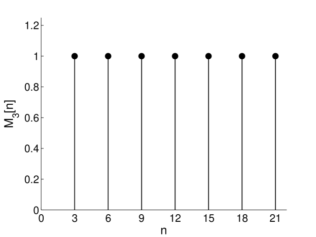
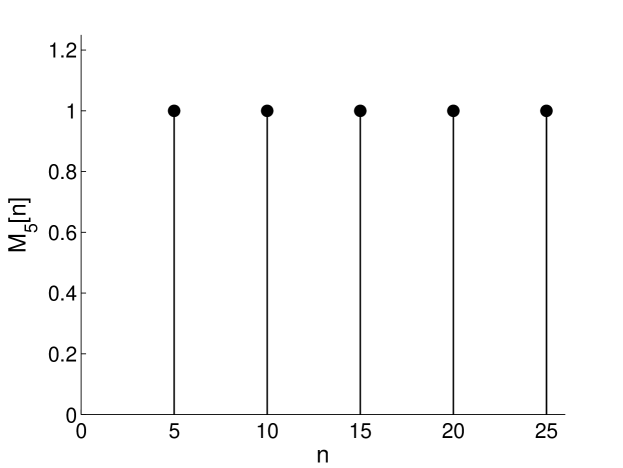
Figure 1: Discrete-time signals $M_{3}[n]$ and $M_{5}[n]$ associated to the sets $M_{3}$ and $M_{5}$, respectively.

3 Density of Particular Sets

In this section, some special sets have their density examined. We focus our attention in three notable sets: (i) set of prime numbers, (ii) Fibonacci sequence, and (iii) set of square-free integers.

3.1 Set of Prime Numbers

Let $P=\{2,3,5,7,11,13,17,19,23,\ldots\}$ be the set of prime numbers.

Proposition 10

The prime numbers set is sparse.

Proof: Utilizing the definition of the prime zeta function, $\zeta^{\prime}(s)\triangleq\sum_{\text{$i:p_{i}$ is prime}}p_{i}^{-s}$, we have that $\operatorname{dens}(P)=\lim_{s\downarrow 1}\frac{\zeta^{\prime}(s)}{\zeta(s)}$. Additionally observe that $\zeta^{\prime}(s)<\infty$ for $s>1$. Taking in account that

$$\ln\zeta(s)=\sum_{k=1}^{\infty}\frac{\zeta^{\prime}(ks)}{k},$$ (59)

for $\epsilon>0$ we have that

$$\ln\zeta(1+\epsilon) =\sum_{k=1}^{\infty}\frac{\zeta^{\prime}(k(1+\epsilon))}{k}$$ (60)

$$=\zeta^{\prime}(1+\epsilon)+\sum_{k=2}^{\infty}\frac{\zeta^{\prime}(k(1+\epsilon))}{k}.$$ (61)

Now consider the following inequalities:

$$0\leq\frac{\zeta^{\prime}(1+\epsilon)}{\zeta(1+\epsilon)} =\frac{\ln\zeta(1+\epsilon)-\sum_{k=2}^{\infty}\frac{\zeta^{\prime}(k(1+\epsilon))}{k}}{\zeta(1+\epsilon)}$$ (62)

$$=\frac{\ln\zeta(1+\epsilon)}{\zeta(1+\epsilon)}-\sum_{k=2}^{\infty}\frac{\frac{\zeta^{\prime}(k(1+\epsilon))}{k}}{\zeta(1+\epsilon)}.$$ (63)

$$\leq\frac{\ln\zeta(1+\epsilon)}{\zeta(1+\epsilon)}.$$ (64)

As $\epsilon\to 0$, we have that $\zeta(1+\epsilon)\to\infty$, therefore

$$\lim_{\epsilon\to 0}\frac{\ln\zeta(1+\epsilon)}{\zeta(1+\epsilon)}=0,$$ (65)

because $\lim_{x\to\infty}\ln(x)/x=0$. Therefore, we can apply the Squeeze Theorem once more, and find that

$$\lim_{\epsilon\to 0}\frac{\zeta^{\prime}(1+\epsilon)}{\zeta(1+\epsilon)}=0.$$ (66)

$\square$

Since the density is zero, it indicates that the associated discrete-time signal $P[n]$, as shown in Figure 2, has null average value.

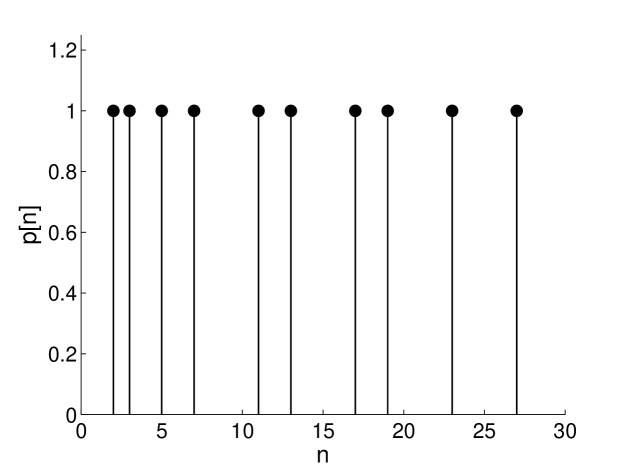
Figure 2: Discrete-time signal $P[n]$ corresponding to the set of prime numbers.

3.2 Fibonacci Sequence

The Fibonacci sequence constitutes another interesting subject of investigation. Fibonacci numbers are constructed according to the following recursive equation $u[n]=u[n-1]+u[n-2]$, $n>1$, for $u[0]=u[1]=1$, where $u[n]$ denotes the nth Fibonacci number [12, p.160]. This procedure results in the Fibonacci set $F=\{1,2,3,5,8,13,21,34,55,\ldots\}$.

Proposition 11

The Fibonacci set is sparse.

Proof: It is known that the sum of the reciprocals of the Fibonacci numbers converges to a constant (reciprocal Fibonacci constant), whose value is approximately $3.35988566\ldots$ [13]. Consequently, for $s>1$, we have that

$$\operatorname{dens}(F)=\lim_{s\downarrow 1}\frac{\sum_{n=2}^{\infty}\frac{1}{u[n]^{s}}}{\zeta(s)}$$ (67)

$$<\lim_{s\downarrow 1}\frac{\sum_{n=1}^{\infty}\frac{1}{u[n]}}{\zeta(s)}=\lim_{s\downarrow 1}\frac{3.35988566\ldots}{\zeta(s)}=0.$$ (68)

$\square$

3.3 Set of Square-free Integers

The set of square-free numbers can be defined as $S\triangleq\{n\in\mathbb{N}\ |\ |\mu(n)|=1\}$, where $\mu(\cdot)$ is the Möbius function, which is given by

$$\mu(n)=\begin{cases}1,&\text{if $n=1$},\\ 0,&\text{if $p^{2}|n$, for some prime number $p$},\\ (-1)^{r},&\text{if $n$ is the product of distinct}\\ &\text{prime numbers.}\end{cases}$$ (69)

Thus the first elements of $S$ are given by $1,2,3,5,6,7,10,11,13,14,15,\ldots$

Proposition 12

The density of the set of square-free integers is $\frac{1}{\zeta(2)}$.

Proof: It is known [14] that $\sum_{n=1}^{\infty}\frac{|\mu(n)|}{n^{s}}=\frac{\zeta(s)}{\zeta(2s)}$, thus it follows easily that:

$$\operatorname{dens}(S) =\lim_{s\downarrow 1}\frac{\sum_{n\in S}\frac{1}{n^{s}}}{\zeta(s)}$$ (70)

$$=\lim_{s\downarrow 1}\frac{\sum_{n=1}^{\infty}\frac{|\mu(n)|}{n^{s}}}{\zeta(s)}$$ (71)

$$=\lim_{s\downarrow 1}\frac{\frac{\zeta(s)}{\zeta(2s)}}{\zeta(s)}=\lim_{s\downarrow 1}\frac{1}{\zeta(2s)}$$ (72)

$$=\frac{1}{\zeta(2)}=\frac{6}{\pi^{2}}.$$ (73)

$\square$

4 Computational Results

Definition 3

Let $A$ be a set of positive integers. The truncated set $A^{T}$ is defined by

$$A^{T}=A\cap\{1,2,3,\ldots,T-1,T\},$$ (74)

where $T$ is a positive integer.

In other words, $A^{T}$ contains the elements of $A$ which are no greater than $T$.

The concept of truncated sets can furnish computational approximations for the numerical value of some densities. Consider, for example, the quantity

$$\operatorname{d}^{\prime}(A^{T})\triangleq\frac{\|A^{T}\|}{\|\mathbb{N}^{T}\|}.$$ (75)

This expression $\operatorname{d}^{\prime}(\cdot)$ can be interpreted in a frequentist way as the ratio between favorable cases and possible cases. Clearly, the asymptotic density can be expressed in terms of $\operatorname{d}^{\prime}(\cdot)$:

$$\operatorname{d}(A)=\lim_{T\to\infty}\operatorname{d}^{\prime}(A^{T}).$$ (76)

In a similar fashion, we can consider a version of the discussed density for truncated sets as defined below. First, observe that discussed density $\operatorname{dens}(\cdot)$ can be expressed as the following double limit

$$\operatorname{dens}(A)=\lim_{s\downarrow 1}\lim_{T\to\infty}\frac{\sum_{n\in A^{T}}\frac{1}{n^{s}}}{\sum_{n=1}^{T}\frac{1}{n^{s}}}.$$ (77)

Restricted to the class of sets for which the above limits can have their order interchanged, we find that

$$\operatorname{dens}(A) =\lim_{T\to\infty}\lim_{s\downarrow 1}\frac{\sum_{n\in A^{T}}\frac{1}{n^{s}}}{\sum_{n=1}^{T}\frac{1}{n^{s}}}$$ (78)

$$=\lim_{T\to\infty}\left(\frac{\sum_{n\in A^{T}}\frac{1}{n}}{\sum_{n=1}^{T}\frac{1}{n}}\right).$$ (79)

Definition 4 (Approximate Density)

The approximate density for a truncated set $A^{T}$ is given by

$$\operatorname{dens}^{\prime}(A^{T})=\frac{\sum_{n\in A^{T}}\frac{1}{n}}{\sum_{n=1}^{T}\frac{1}{n}}.$$ (80)

Again, whenever the limit order of Equation 77 can be interchanged, we have that

$$\operatorname{dens}(A)=\lim_{T\to\infty}\operatorname{dens}^{\prime}(A^{T}).$$ (81)

The quantity $\operatorname{dens}^{\prime}(\cdot)$ furnishes a computationally feasible way to investigate the behavior of $\operatorname{dens}(\cdot)$.

In the following, we obtain computational approximations for the asymptotic density and the discussed density. The approximate densities are numerically evaluated as $T$ increases in the range from 1 to 1000. Now we investigate (i) arithmetic progressions, (ii) the set of prime numbers, and (iii) the Fibonacci sequence.

4.1 Arithmetic Progressions

Considering an arithmetic progressions $M_{q}$, we have that:

$$\operatorname{d}(M_{q})=\lim_{T\to\infty}\operatorname{d}^{\prime}(M_{q}^{T})=\frac{1}{q},$$ (82)

and

$$\operatorname{dens}(M_{q})=\lim_{T\to\infty}\operatorname{dens}^{\prime}(M_{q}^{T}).$$ (83)

Both quantities limits converge to the same quantity $1/q$. Intuitively, we have that the chance of “selecting” a multiple of $q$ among all integers is $1/q$. This is exactly the density of $M_{q}$. Figure 3 shows the result of computational calculations of $\operatorname{d}^{\prime}(\cdot)$ and $\operatorname{dens}^{\prime}(\cdot)$ for $M_{2}^{T}$.

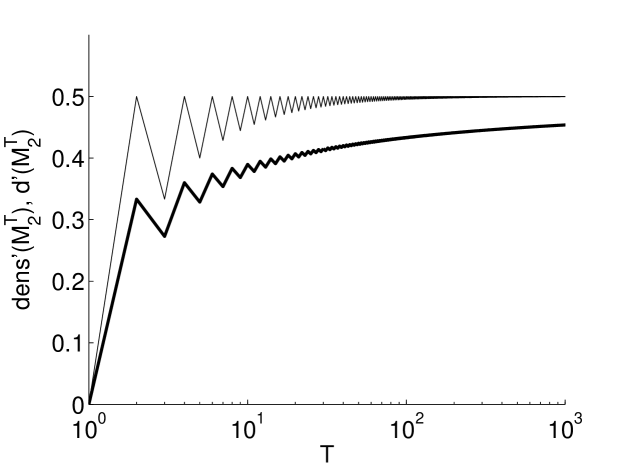
Figure 3: Computational result for the approximate density for the truncated prime set $M_{2}^{T}$, according to (i) the function $\operatorname{dens}^{\prime}(P^{T})$ (bold curve), and (ii) the function $\operatorname{d}^{\prime}(P^{T})$ (thin line). Observe the convergence to $1/2$.

4.2 Prime numbers sets

Consider the truncated set of prime numbers $P^{T}=\{p:\text{$p$ is a prime},p<T)$. One may easily compute both $\operatorname{d}^{\prime}(P^{T})$ and $\operatorname{dens}^{\prime}(P^{T})$ for any finite $T$.

An alternative path for the estimation of $\operatorname{d}^{\prime}(P^{T})=\frac{\pi(T)}{T}$, where the function $\pi(x)$ represents the number of primes that do not exceed $x$, is to utilize the approximation for $\pi(T)$ given by the Prime Number Theorem [12, 15, p.336]:

$$\pi(T)\approx\operatorname{li}(T),$$ (84)

where $\operatorname{li}(\cdot)$ denotes the logarithmic integral [16]. The curves displayed in Figure 4 correspond to the calculation of $\operatorname{dens}^{\prime}(P^{T})$, $\operatorname{d}^{\prime}(P^{T})$ and $\operatorname{li}(T)/T$. As expected, all curves decay to zero.

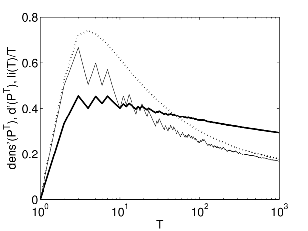
Figure 4: Computational result for the approximate density for the truncated prime set $P^{T}$, according to (i) the function $\operatorname{dens}^{\prime}(P^{T})$ (bold curve), (ii) the function $\operatorname{d}^{\prime}(P^{T})$ (thin line), and (iii) the approximation based on the Prime Number Theorem (dotted line).

4.3 Fibonacci Sequence

Now consider the truncated Fibonacci set $F^{T}=\{1,2,3,5,8,13,21,\ldots,T\}$. The result of calculating

$$\operatorname{d}^{\prime}(F^{T})=\frac{\|F^{T}\|}{\|\mathbb{N}^{T}\|}$$ (85)

and

$$\operatorname{dens}^{\prime}(F^{T})=\frac{\sum_{n\in F^{T}}\frac{1}{n}}{\sum_{n=1}^{T}\frac{1}{n}},$$ (86)

are shown in Figure 5. Both curves tend to zero as $T$ grows. This fact is expected since we have already verified that $\operatorname{dens}(F)=0$. The small convergence rate of $\operatorname{dens}^{\prime}(\cdot)$ is typical of problems that deal with the harmonic series.

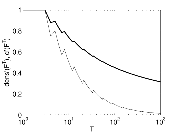
Figure 5: Density of the truncated Fibonacci set: $\operatorname{dens}^{\prime}(F^{T})$ (bold line) and $\operatorname{d}^{\prime}(F^{T})$ (thin line).

5 Conclusion

A density for infinite sets of integers was investigated. It was shown that the suggested density shares several properties of usual probability. A computational simulation of the proposed approximate density for finite sets was addressed. An open topic is the characterization of sets for which the limiting value of the approximate density equals their density.

References

- [1] J. P. Bell and S. N. Burris, “Dirichlet density extends global asymptotic density in multiplicative systems,” Preprint published at htt://www.math.uwaterloo.ca/~snburris/htdocs/MYWORKS/, 2006.
- [2] R. L. Duncan, “Some continuity properties of the Schnirelmann density,” Pacific Journal of Mathematics, vol. 26, no. 1, pp. 57–58, 1968.
- [3] ——, “Some continuity properties of the Schnirelmann density II,” Pacific Journal of Mathematics, vol. 32, no. 1, pp. 65–67, 1970.
- [4] P. Erdös, “On the density of some sequences of integers,” Bulletin of the American Mathematical Society, vol. 54, no. 8, pp. 685–692, Aug. 1948.
- [5] H. Davenport and P. Erdös, “On sequences of positive integers,” Journal of the Indian Mathematical Society, vol. 15, pp. 19–24, 1951.
- [6] R. Ahlswede and L. H. Khachatrian, “Number theoretic correlation inequalities for Dirichlet densities,” Journal of Number Theory, vol. 63, pp. 34–46, 1997.
- [7] I. Niven and H. S. Zickerman, An Introduction to the Theory of Numbers. John Wiley & Sons, Inc., 1960.
- [8] I. S. Gradshteyn and I. M. Ryzhik, Table of Integrals, Series, and Products, 4th ed. New York: Academic Press, 1965.
- [9] P. Erdös, R. R. Hall, and G. Tenebaum, “On the densities of sets of multiples,” Journal für die reine und angewandte Mathematik, vol. 454, pp. 119–141, 1994.
- [10] W. Rudin, Real and Complex Analysis. McGraw-Hill, 1970.
- [11] S. Abbott, Understanding Analysis. Springer, 2001.
- [12] D. M. Burton, Elementary Number Theory. McGraw-Hill, 1998.
- [13] R. André-Jeannin, “Irrationalité de la somme des inverses de certaines suites récurrentes,” in C. R. Acad. Sci. Paris Sér. I Math., vol. 308, 1989, pp. 539–541.
- [14] M. R. Schroeder, Number Theory in Science and Communication, 3rd ed., ser. Springer Series in Information Sciences, T. S. Huang, T. Kohonen, and M. R. Schroeder, Eds. Springer, 1997, vol. 7.
- [15] H. Riesel, Prime Numbers and Computer Methods for Factorization. Birkhäuser, 1985.
- [16] M. Abramowitz and I. Segun, Handbook of Mathematical Functions. New York: Dover, 1968.