Analysis of classifiers’ robustness to adversarial perturbations
Analysis of classifiers’ robustness to adversarial perturbations
Abstract
The goal of this paper is to analyze an intriguing phenomenon recently discovered in deep networks, namely their instability to adversarial perturbations (Szegedy et al, 2014). We provide a theoretical framework for analyzing the robustness of classifiers to adversarial perturbations, and show fundamental upper bounds on the robustness of classifiers. Specifically, we establish a general upper bound on the robustness of classifiers to adversarial perturbations, and then illustrate the obtained upper bound on two practical classes of classifiers, namely the linear and quadratic classifiers. In both cases, our upper bound depends on a distinguishability measure that captures the notion of difficulty of the classification task. Our results for both classes imply that in tasks involving small distinguishability, no classifier in the considered set will be robust to adversarial perturbations, even if a good accuracy is achieved. Our theoretical framework moreover suggests that the phenomenon of adversarial instability is due to the low flexibility of classifiers, compared to the difficulty of the classification task (captured mathematically by the distinguishability measure). Moreover, we further show the existence of a clear distinction between the robustness of a classifier to random noise and its robustness to adversarial perturbations. Specifically, the former is shown to be larger than the latter by a factor that is proportional to (with being the signal dimension) for linear classifiers. This result gives a theoretical explanation for the discrepancy between the two robustness properties in high dimensional problems, which was empirically observed in Szegedy et al (2014) in the context of neural networks. To the best of our knowledge, our results provide the first theoretical work that addresses the phenomenon of adversarial instability recently observed for deep networks. We finally show experimental results on controlled and real-world data that confirm the theoretical analysis and extends its spirit to more complex classification schemes.
1 Introduction
State-of-the-art deep networks have recently been shown to be surprisingly unstable to adversarial perturbations (Szegedy et al, 2014). Unlike random noise, adversarial perturbations are minimal perturbations that are sought to switch the estimated label of the classifier. On vision tasks, the results of Szegedy et al (2014) have shown that perturbations that are hardly perceptible to the human eye are sufficient to change the decision of a deep network, even if the classifier has a performance that is close to the human visual system. This surprising instability raises interesting theoretical questions that we initiate in this paper. What causes classifiers to be unstable to adversarial perturbations? Are deep networks the only classifiers that have such unstable behaviour? Is it at all possible to design training algorithms to build deep networks that are robust or is the instability to adversarial noise an inherent feature of all deep networks? Can we quantify the difference between random noise and adversarial noise? Providing theoretical answers to these questions is crucial in order to achieve the goal of building classifiers that are robust to adversarial hostile perturbations.
In this paper, we introduce a framework to formally study the robustness of classifiers to adversarial perturbations in the binary setting. We provide a general upper bound on the robustness of classifiers to adversarial perturbations, and then illustrate and specialize the obtained upper bound for the families of linear and quadratic classifiers. In both cases, our results show the existence of a fundamental limit on the robustness to adversarial perturbations. This limit is expressed in terms of a distinguishability measure between the classes, which depends on the considered family of classifiers. Specifically, for linear classifiers, the distinguishability is defined as the distance between the means of the two classes, while for quadratic classifiers, it is defined as the distance between the matrices of second order moments of the two classes. For both classes of functions, our upper bound on the robustness is valid for all classifiers in the family independently of the training procedure, and we see the fact that the bound is independent of the training procedure as a strength. This result has the following important implication: in difficult classification tasks involving a small value of distinguishability, any classifier in the set with low misclassification rate is vulnerable to adversarial perturbations. Importantly, the distinguishability parameter related to quadratic classifiers is much larger than that of linear classifiers for many datasets of interest, and suggests that it is harder to find adversarial examples for more flexible classifiers. We further compare the robustness to adversarial perturbations of linear classifiers to the more traditional notion of robustness to random uniform noise. The latter robustness is shown to be larger than the former by a factor of (with the dimension of input signals), thereby showing that in high dimensional classification tasks, linear classifiers can be robust to random noise even for small values of the distinguishability. We illustrate the newly introduced concepts and our theoretical results on a running example used throughout the paper. We complement our theoretical analysis with experimental results, and show that the intuition obtained from the theoretical analysis also holds for more complex classifiers.
The phenomenon of adversarial instability has recently attracted a lot of attention from the deep network community. Following the original paper (Szegedy et al, 2014), several attempts have been made to make deep networks robust to adversarial perturbations (Chalupka et al, 2014; Gu and Rigazio, 2014). Moreover, a distinct but related phenomenon has been explored in Nguyen et al (2014). Closer to our work, the authors of (Goodfellow et al, 2015) provided an empirical explanation of the phenomenon of adversarial instability, and designed an efficient method to find adversarial examples. Specifically, contrarily to the original explanation provided in Szegedy et al (2014), the authors argue that it is the “linear” nature of deep nets that causes the adversarial instability. Instead, our paper adopts a rigorous mathematical perspective to the problem of adversarial instability and shows that adversarial instability is due to the low flexibility of classifiers compared to the difficulty of the classification task.
Our work should not be confused with works on the security of machine learning algorithms under adversarial attacks (Biggio et al, 2012; Barreno et al, 2006; Dalvi et al, 2004). These works specifically study attacks that manipulate the learning system (e.g., change the decision function by injecting malicious training points), as well as defense strategies to counter these attacks. This setting significantly differs from ours, as we examine the robustness of a fixed classifier to adversarial perturbations (that is, the classifier cannot be manipulated). The stability of learning algorithms has also been defined and extensively studied in (Bousquet and Elisseeff, 2002; Lugosi and Pawlak, 1994). Again, this notion of stability differs from the one studied here, as we are interested in the robustness of fixed classifiers, and not of learning algorithms.
The construction of learning algorithms that achieve robustness of classifiers to data corruption has been an active area of research in machine learning and robust optimization (see e.g., Caramanis et al (2012) and references therein). For a specific disturbance model on the data samples, the robust optimization approach for constructing robust classifiers seeks to minimize the worst possible empirical error under such disturbances (Lanckriet et al, 2003; Xu et al, 2009). It is shown that, for many disturbance models, the desired objective function can be written as a tractable convex optimization problem. Our work studies the robustness of classifiers from a different perspective; we establish upper bounds on the robustness of classifiers independently of the learning algorithms. That is, using our bounds, we can certify the instability of a class of classifiers to adversarial perturbations, independently of the learning mechanism. In other words, while algorithmic and optimization aspects of robust classifiers have been studied in the above works, we focus on fundamental limits on the adversarial robustness of classifiers that are independent of the learning scheme.
The paper is structured as follows: Sec. 2 introduces the problem setting. In Sec. 3, we introduce a running example that is used throughout the paper. We introduce in Sec. 4 a theoretical framework for studying the robustness to adversarial perturbations. In the following two sections, two case studies are analyzed in detail. The robustness of linear classifiers (to adversarial and random noise) is studied in Sec. 5. In Sec. 6, we study the adversarial robustness of quadratic classifiers. Experimental results illustrating our theoretical analysis are given in Section 7. Proofs and additional discussion on the choice of the norms to measure perturbations are finally deferred to the appendix.
2 Problem setting
We first introduce the framework and notations that are used for analyzing the robustness of classifiers to adversarial and uniform random noise. We restrict our analysis to the binary classification task, for simplicity. We expect similar conclusions for the multi-class case, but we leave that for future work. Let denote the probability measure on of the data points that we wish to classify, and be the label of a point . The distribution is assumed to be of bounded support. That is, , with for some . We further denote by and the distributions of class and class in , respectively. Let be an arbitrary classification function. The classification rule associated to is simply obtained by taking the sign of . The performance of a classifier is usually measured by its risk, defined as the probability of misclassification according to :
where .
The focus of this paper is to study the robustness of classifiers to adversarial perturbations in the ambient space . Given a datapoint sampled from , we denote by the norm of the smallest perturbation that switches the sign111We make the assumption that a perturbation that satisfies the equality flips the estimated label of . of :
| (1) |
Here, we use the norm to quantify the perturbation; we refer the reader to Appendix C for a discussion of the norm choice. Unlike random noise, the above definition corresponds to a minimal noise, where the perturbation is sought to flip the estimated label of . This justifies the adversarial nature of the perturbation. It is important to note that, while is a datapoint sampled according to , the perturbed point is not required to belong to the dataset (i.e., can be outside the support of ). The robustness to adversarial perturbation of is defined as the average of over all :
| (2) |
In words, is defined as the average norm of the minimal perturbations required to flip the estimated labels of the datapoints. Note that is a property of both the classifier and the distribution , but it is independent of the true labels of the datapoints .222In that aspect, our definition slightly differs from the one proposed in Szegedy et al (2014), which defines the robustness to adversarial perturbations as the average of the norms of the minimal perturbations required to misclassify all datapoints. As our notion of robustness is larger, the upper bounds derived in our paper also directly apply for the definition of robustness in Szegedy et al (2014). Moreover, it should be noted that is different from the margin considered by SVMs. In fact, SVM margins are traditionally defined as the minimal distance to the (linear) boundary over all training points, while is defined as the average distance to the boundary over all training points. In addition, distances in our case are measured in the input space, while the margin is defined in the feature space for kernel SVMs.
In this paper, we also study the robustness of classifiers to random uniform noise, that we define as follows. For a given , let
| (3) | ||||
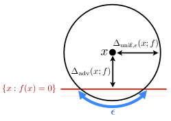
where denotes the uniform measure on the sphere centered at and of radius in . In words, denotes the maximal radius of the sphere centered at , such that perturbed points sampled uniformly at random from this sphere are classified similarly to with high probability. An illustration of and is given in Fig. 1. Similarly to adversarial perturbations, the point will lie outside the support of , in general. Note moreover that provides an upper bound on , for all . The -robustness of to random uniform noise is defined by:
| (4) |
We summarize the quantities of interest in Table 1.
| Quantity | Definition | Dependence |
|---|---|---|
| Risk | ||
| Robustness to adversarial perturbations | ||
| Robustness to random uniform noise |
3 Running example
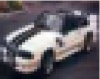
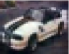
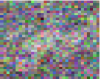
We introduce in this section a running example used throughout the paper to illustrate the notion of adversarial robustness, and highlight its difference with the notion of risk. We consider a binary classification task on square images of size . Images of class (resp. class ) contain exactly one vertical line (resp. horizontal line), and a small constant positive number (resp. negative number ) is added to all the pixels of the images. That is, for class (resp. ) images, background pixels are set to (resp. ), and pixels belonging to the line are equal to (resp. ). Fig. 2 illustrates the classification problem for . The number of datapoints to classify is .
Clearly, the most relevant concept (in terms of visual appearance) that permits to separate the two classes is the orientation of the line (i.e., horizontal vs. vertical). The bias of the image (i.e., the sum of all its pixels) is also a valid concept for this task, as it separates the two classes, despite being much more difficult to detect visually. The class of an image can therefore be correctly estimated from its orientation or from the bias. Let us first consider the linear classifier defined by
| (5) |
where is the vector of size whose entries are all equal to , and is the vectorized image, exploits the difference of bias between the two classes and achieves a perfect classification accuracy for all . Indeed, a simple computation gives (resp. ) for class (resp. class ) images. Therefore, the risk of is . It is important to note that only achieves zero risk because it captures the bias, but fails to distinguish between the images based on the orientation of the line. Indeed, when , the datapoints are not linearly separable. Despite its perfect accuracy for any , is not robust to small adversarial perturbations when is small, as a minor perturbation of the bias switches the estimated label. Indeed, a simple computation gives ; therefore, the adversarial robustness of can be made arbitrarily small by choosing to be small enough. More than that, among all linear classifiers that satisfy , is the one that maximizes (as we show later in Section 5). Therefore, all zero-risk linear classifiers are not robust to adversarial perturbations, for this classification task.
Unlike linear classifiers, a more flexible classifier that correctly captures the orientation of the lines in the images will be robust to adversarial perturbation, unless this perturbation significantly alters the image and modifies the direction of the line. To illustrate this point, we compare the adversarial robustness of to that of a second order polynomial classifier that achieves zero risk in Fig. 3, for .333We postpone the detailed analysis of to Section 6. While a hardly perceptible change of the image is sufficient to switch the estimated label for the linear classifier, the minimal perturbation for is one that modifies the direction of the line, to a great extent.


The above example highlights several important facts, which are summarized as follows:
-
•
Risk and adversarial robustness are two distinct properties of a classifier. While , is definitely not robust to small adversarial perturbations.444The opposite is also possible, since a constant classifier (e.g., for all ) is clearly robust to perturbations, but does not achieve good accuracy. This is due to the fact that only captures the bias in the images and ignores the orientation of the line.
-
•
To capture orientation (i.e., the most visual concept), one has to use a classifier that is flexible enough for the task. Unlike the class of linear classifiers, the class of polynomial classifiers of degree correctly captures the line orientation, for .
-
•
The robustness to adversarial perturbations provides a quantitative measure of the strength of a concept. Since , one can confidently say that the concept captured by is stronger than that of , in the sense that the essence of the classification task is captured by , but not by (while they are equal in terms of misclassification rate). In general classification problems, the quantity provides a natural way to evaluate and compare the learned concept; larger values of indicate that stronger concepts are learned, for comparable values of the risk.
As illustrated in the above toy example, the robustness to adversarial perturbations is key to assess the strength of a concept. In real-world classification tasks, weak concepts correspond to partial information about the classification task (which are possibly sufficient to achieve a good accuracy), while strong concepts capture the essence of the classification task.
4 Upper limit on the adversarial robustness
We now introduce our theoretical framework for analyzing the robustness to adversarial perturbations. We first present a key assumption on the classifier for the analysis of adversarial robustness.
Assumption (A). There exist and such that, for all ,
| (6) | ||||
where and (resp. ) is the set of points such that (resp. ):
In words, the assumption (A) states that for any datapoint , the residual (resp. ) can be used to bound the distance from to a datapoint classified (resp. ).
Bounds of the form Eq. (6) have been established for various classes of functions since the early of work of Lojasiewicz (Łojasiewicz, 1961) in algebraic geometry and have found applications in areas such as mathematical optimization (Pang, 1997; Lewis and Pang, 1998). For example, Lojasiewicz (Łojasiewicz, 1961) and later (Luo and Pang, 1994) have shown that, quite remarkably, assumption (A) holds for the general class of analytic functions. In (Ng and Zheng, 2003), (A) is shown to hold with for piecewise linear functions. In (Luo and Luo, 1994), error bounds on polynomial systems are studied. Proving inequality (6) with explicit constants and for different classes of functions is still an active area of research (Li et al, 2014). In Sections 5 and 6, we provide examples of function classes for which (A) holds, and explicit formulas for the parameters and .
The following result establishes a general upper bound on the robustness to adversarial perturbations:
Lemma 4.1.
Let be an arbitrary classifier that satisfies (A) with parameters . Then,
The proof can be found in Appendix A.1. The above result provides an upper bound on the adversarial robustness that depends on the risk of the classifier, as well as a measure of the separation between the expectations of the classifier values computed on distribution and . This result is general, as we only assume that satisfies assumption . In the next two sections, we apply Lemma 4.1 to two classes of classifiers, and derive interpretable upper bounds in terms of a distinguishibality measure (that depends only on the dataset) which quantifies the notion of difficulty of a classification task. Studying the general result in Lemma 4.1 through two practical classes of classifiers shows the implications of such a fundamental limit on the adversarial robustness, and illustrates the methodology for deriving class-specific and practical upper bounds on adversarial robustness from the general upper bound.
5 Robustness of linear classifiers to adversarial and random perturbations
The goal of this section is two-fold; first, we specialize Lemma 4.1 to the class of linear functions, and derive interpretable upper bounds on the robustness of classifiers to adversarial perturbations (Section 5.1). Then, we derive a formal relation between the robustness of linear classifiers to adversarial robustness, and the robustness to random uniform noise (Section 5.2).
5.1 Adversarial perturbations
We define the classification function . Note that any linear classifier for which is a trivial classifier that assigns the same label to all points, and we therefore assume that .
We first show that the family of linear classifiers satisfies assumption (A), with explicit parameters and .
Lemma 5.1.
Assumption (A) holds for linear classifiers with and .
Proof.
Let be such that , and the goal is to prove that (the other inequality can be handled in a similar way). We have . . ∎
Using Lemma 4.1, we now derive an interpretable upper bound on the robustness to adversarial perturbations. In particular, the following theorem bounds from above in terms of the first moments of the distributions and , and the classifier’s risk:
Theorem 5.2.
Let such that . Then,
| (7) |
In the balanced setting where , and if the intercept the following inequality holds:
| (8) |
Proof.
Using Lemma 4.1 with and , we have
| (9) |
Observe that
-
i.
using Cauchy-Schwarz inequality.
-
ii.
using the assumption ,
-
iii.
.
By plugging the three inequalities in Eq. (9), we obtain the desired result in Eq. (7).
When , and the intercept , inequality (iii) can be tightened to , and directly leads to the stated result Eq. (8). ∎
Our upper bound on depends on the difference of means , which measures the distinguishability between the classes. Note that this term is classifier-independent, and is only a property of the classification task. The only dependence on in the upper bound is through the risk . Thus, in classification tasks where the means of the two distributions are close (i.e., is small), any linear classifier with small risk will necessarily have a small robustness to adversarial perturbations. Note that the upper bound logically increases with the risk, as there clearly exist robust linear classifiers that achieve high risk (e.g., constant classifier). Fig. 4 (a) pictorially represents the vs diagram as predicted by Theorem 5.2. Each linear classifier is represented by a point on the – diagram, and our result shows the existence of a region that linear classifiers cannot attain.
Quite importantly, in many interesting classification problems, the quantity is small due to large intra-class variability (e.g., due to complex intra-class geometric transformations in computer vision applications). Therefore, even if a linear classifier can achieve a good classification performance on such a task, it will not be robust to small adversarial perturbations. In simple tasks involving distributions with significantly different averages, it is likely that there exists a linear classifier that can separate correctly the classes, and have a large robustness to adversarial perturbations.


5.2 Random uniform noise
We now examine the robustness of linear classifiers to random uniform noise. The following theorem compares the robustness of linear classifiers to random uniform noise with their robustness to adversarial perturbations.
Theorem 5.3.
Let . For any , we have the following bounds on :
| (10) | ||||
| (11) |
with , and .
The proof can be found in appendix A.2. In words, behaves as for linear classifiers (for constant ). Linear classifiers are therefore more robust to random noise than adversarial perturbations, by a factor of . In typical high dimensional classification problems, this shows that a linear classifier can be robust to random noise even if is small. Note moreover that our result is tight for , as we get .
Our results can be put in perspective with the empirical results of Szegedy et al (2014), that showed a large gap between the two notions of robustness on neural networks. Our analysis provides a confirmation of this high dimensional phenomenon on linear classifiers.
5.3 Illustration of the results on the running example
We now illustrate our theoretical results on the example of Section 3. In this case, we have . By using Theorem 5.2, any zero-risk linear classifier satisfies . As we choose , accurate linear classifiers are therefore not robust to adversarial perturbations for this task. We note that (defined in Eq.(5)) achieves the upper bound and is therefore the most robust accurate linear classifier one can get, as it can easily be checked that . In Fig. 4 (b) the exact vs curve is compared to our theoretical upper bound555The exact curve is computed using a bruteforce approach., for , and a bias . Besides the zero-risk case where our upper bound is tight, the upper bound is reasonably close to the exact curve for other values of the risk (despite not being tight).
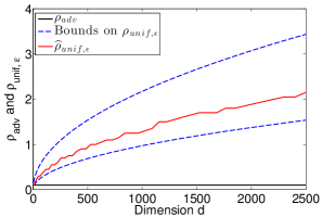
We now focus on the robustness to uniform random noise of . For various values of , we compute the upper and lower bounds on the robustness to random uniform noise (Theorem 5.3) of , where we fix to . In addition, we compute a simple empirical estimate of the robustness to random uniform noise of (see Sec. 7 for details on the computation of this estimate). The results are illustrated in Fig. 5. While the adversarial noise robustness is constant with the dimension (equal to , as and ), the robustness to random uniform noise increases with . For example, for , the value of is at least times larger than the adversarial robustness . In high dimensions, a linear classifier is therefore much more robust to random uniform noise than adversarial noise.
6 Adversarial robustness of quadratic classifiers
In this section, we derive specialized upper bounds on the robustness to adversarial perturbations of quadratic classifers using Lemma 4.1.
6.1 Analysis of adversarial perturbations
We study the robustness to adversarial perturbations of quadratic classifiers of the form , where is a symmetric matrix. Besides the practical use of quadratic classifiers in some applications (Goldberg and Elhadad, 2008; Chang et al, 2010), they represent a natural extension of linear classifiers. The study of linear vs. quadratic classifiers provides insights into how adversarial robustness depends on the family of considered classifiers. Similarly to the linear setting, we exclude the case where is a trivial classifier that assigns a constant label to all datapoints. That is, we assume that satisfies
| (12) |
where and are the smallest and largest eigenvalues of . We moreover impose that the eigenvalues of satisfy
| (13) |
for some constant value . This assumption imposes an approximate symmetry around of the extremal eigenvalues of , thereby disallowing a large bias towards any of the two classes.
We first show that the assumption (A) is satisfied for quadratic classifiers, and derive explicit formulas for and .
Lemma 6.1.
Assumption (A) holds for the class of quadratic classifiers where , with , and ,
Proof.
Let be such that , and the goal is to prove that (the other inequality can be handled in a similar way). Assume without loss of generality that is diagonal (this can be done using an appropriate change of basis). Let . We have . By setting for all and , (where if and otherwise) we have
Hence, . ∎
The following result builds on Lemma 4.1 and bounds the adversarial robustness of quadratic classifiers as a function of the second order moments of the distribution and the risk.
Theorem 6.2.
Proof.
The class of classifiers under study satisfies assumption (A) with , and (see Lemma 6.1). By applying Lemma 4.1, we have
Observe that
-
i.
using the generalized Cauchy-Schwarz inequality, where and denote respectively the spectral and nuclear matrix norms.
-
ii.
,
-
iii.
.
Applying these three inequalities, we obtain
∎
In words, the upper bound on the adversarial robustness depends on a distinguishability measure, defined by , and the classifier’s risk. In difficult classification tasks, where is small, any quadratic classifier with low risk that satisfies our assumptions in Eq. (12, 13) is not robust to adversarial perturbations.
It should be noted that, while the distinguishability is measured with the distance between the means of the two distributions in the linear case, it is defined here as the difference between the second order moments matrices . Therefore, in classification tasks involving two distributions with close means, and different second order moments, any zero-risk linear classifier will not be robust to adversarial noise, while zero-risk and robust quadratic classifiers are a priori possible according to our upper bound in Theorem 6.2. This suggests that robustness to adversarial perturbations can be larger for more flexible classifiers, for comparable values of the risk.
6.2 Illustration of the results on the running example
We now illustrate our results on the running example of Section 3, with . In this case, a simple computation gives . This term is significantly larger than the difference of means (equal to ), and there is therefore hope to have a quadratic classifier that is accurate and robust to small adversarial perturbations, according to Theorem 6.2. In fact, the following quadratic classifier
outputs for vertical images, and for horizontal images (independently of the bias ). Therefore, achieves zero risk on this classification task, similarly to . The two classifiers however have different robustness properties to adversarial perturbations. Using straightforward calculations, it can be shown that , for any value of (see Appendix B for more details). For small values of , we therefore get . This result is intuitive, as differentiates the images from their orientation, unlike that uses the bias to distinguish them. The minimal perturbation required to switch the estimated label of is therefore one that modifies the direction of the line, while a hardly perceptible perturbation that modifies the bias is enough to flip the label for . This explains the result originally illustrated in Fig. 3.
7 Experimental results
7.1 Setting
In this section, we illustrate our results on practical classification examples. Specifically, through experiments on real data, we seek to confirm the identified limit on the robustness of classifiers, and we show the large gap between adversarial and random robustness on real data. We also study more general classifiers to suggest that the trends obtained with our theoretical results are not limited to linear and quadratic classifiers.
Given a binary classifier , and a datapoint , we use an approach close to that of Szegedy et al (2014) to approximate . Specifically, we perform a line search to find the maximum for which the minimizer of the following problem satisfies :
where we set . The above problem (for fixed) is solved with a subgradient procedure, and we denote by the obtained solution.666This procedure is not guaranteed to provide the optimal solution (for arbitrary classifiers ), as the problem is clearly non convex. Strictly speaking, the optimization procedure is only guaranteed to provide an upper bound on . The empirical robustness to adversarial perturbations is then defined by , where denote the training points. To evaluate the robustness of , we compare to the following quantity:
| (14) |
It represents the average norm of the minimal perturbation required to “transform” a training point to a training point of the opposite class, and can be seen as a distance measure between the two classes. The quantity therefore provides a baseline for comparing the robustness to adversarial perturbations, and we say that is not robust to adversarial perturbations when . We also compare the adversarial robustness of the classifiers with their robustness to random uniform noise. We estimate using a line search procedure that finds the largest for which the condition
is satisfied, where are iid samples from the sphere . By calling this estimate , the robustness of to uniform random noise is the empirical average over all training points, i.e., . In the experiments, we set , and .777We compute the robustness to uniform random noise of all classifiers, except RBF-SVM, as this classifier is often asymmetric, assigning to one of the classes “small pockets” in the ambient space, and the rest of the space is assigned to the other class. In these cases, the robustness to uniform random noise can be equal to infinity for one of the classes, for a given .
7.2 Binary classification using SVM
We perform experiments on several classifiers: linear SVM (denoted L-SVM), SVM with polynomial kernels of degree (denoted poly-SVM ()), and SVM with RBF kernel with a width parameter (RBF-SVM()). To train the classifiers, we use the efficient Liblinear (Fan et al, 2008) and LibSVM (Chang and Lin, 2011) implementations, and we fix the regularization parameters using a cross-validation procedure.
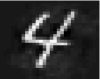
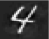
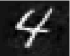
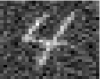
We first consider a classification task on the MNIST handwritten digits dataset (LeCun et al, 1998). We consider a digit “4” vs. digit “5” binary classification task, with and randomly chosen images for training and testing, respectively. In addition, a small random translation is applied to all images, and the images are normalized to be of unit Euclidean norm. Table 2 reports the accuracy of the different classifiers, and their robustness to adversarial and random perturbations. Despite the fact that L-SVM performs fairly well on this classification task (both on training and testing), it is highly non robust to small adversarial perturbations. Indeed, is one order of magnitude smaller than . Visually, this translates to an adversarial perturbation that is hardly perceptible. The instability of the linear classifier to adversarial perturbations is not surprising in the light of Theorem 5.2, as the distinguishability term is small (see Table 4). In addition to improving the accuracy, the more flexible classifiers are also more robust to adversarial perturbations, as predicted by our theoretical analysis. That is, the third order classifier is slightly more robust than the second order one, and RBF-SVM with small width is more robust than with . Note that controls the flexibility of the classifier in a similar way to the degree in the polynomial kernel. Interestingly, in this relatively easy classification task, RBF-SVM(0.1) achieves both a good performance, and a high robustness to adversarial perturbations. Concerning the robustness to random uniform noise, the results in Table 2 confirm the large gap between adversarial and random robustness for the linear classifier, as predicted by Theorem 5.3. Moreover, the results suggest that this gap is maintained for polynomial SVM. Fig. 6 illustrates the robustness of the different classifiers on an example image.
| Model | Train error (%) | Test error (%) | ||
|---|---|---|---|---|
| L-SVM | 4.8 | 7.0 | 0.08 | 0.97 |
| poly-SVM() | 0 | 1 | 0.19 | 2.15 |
| poly-SVM() | 0 | 0.6 | 0.24 | 2.51 |
| RBF-SVM() | 0 | 1.1 | 0.16 | - |
| RBF-SVM() | 0 | 0.5 | 0.32 | - |


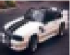
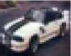
We now turn to a natural image classification task, with images taken from the CIFAR-10 database (Krizhevsky and Hinton, 2009). The database contains classes of RGB images. We restrict the dataset to the first two classes (“airplane” and “automobile”), and consider a subset of the original data, with images for training, and for testing. Moreover, all images are normalized to be of unit Euclidean norm. Compared to the first dataset, this task is more difficult, as the variability of the images is much larger than for digits. We report the results in Table 3. It can be seen that all classifiers are not robust to adversarial perturbations for this experiment, as . Despite that, all classifiers (except L-SVM) achieve an accuracy around , and a training accuracy above , and are robust to uniform random noise. Fig. 7 illustrates the robustness to adversarial and random noise of the learned classifiers, on an example image of the dataset. Compared to the digits dataset, the distinguishability measures for this task are smaller (see Table 4). Our theoretical analysis therefore predicts a lower limit on the adversarial robustness of linear and quadratic classifiers for this task (even though the bound for quadratic classifiers is far from the achieved robustness of poly-SVM(2) in this example).
| Model | Train error (%) | Test error (%) | ||
|---|---|---|---|---|
| L-SVM | 14.5 | 21.3 | 0.04 | 0.94 |
| poly-SVM() | 4.2 | 15.3 | 0.03 | 0.73 |
| poly-SVM() | 4 | 15 | 0.04 | 0.89 |
| RBF-SVM() | 7.6 | 16 | 0.04 | - |
| RBF-SVM() | 0 | 13.1 | 0.06 | - |


| Quantity | Definition | Digits | Natural images |
|---|---|---|---|
| Distance between classes | (see Eq. (14)) | 0.72 | 0.39 |
| Distinguishability (linear class.) | 0.14 | 0.06 | |
| Distinguishability (quadratic class.) | 1.4 | 0.87 |
The instability of all classifiers to adversarial perturbations on this task suggests that the essence of the classification task was not correctly captured by these classifiers, even if a fairly good test accuracy is reached. To reach better robustness, two possibilities exist: use a more flexible family of classifiers (as our theoretical results suggest that more flexible families of classifiers achieve better robustness), or use a better training algorithm for the tested nonlinear classifiers. The latter solution seems possible, as the theoretical limit for quadratic classifiers suggests that there is still room to improve the robustness of these classifiers.
7.3 Multiclass classification using CNN
Since our theoretical results suggest that more flexible classifiers achieve better robustness to adversarial perturbations in the binary case, we now explore empirically whether the same intuitions hold in scenarios that depart from the theory in two different ways: (i) we consider multiclass classification problems, and (ii) we consider convolutional neural network architectures. While classifiers’ flexibility is relatively well quantified for polynomial classifiers by the degree of the polynomials, this is not straightforward to do for neural network architectures. In this section, we examine the effect of breadth and depth on the robustness to adversarial perturbations of classifiers.
We perform experiments on the multiclass CIFAR-10 classification task, and use the recent method in (Moosavi-Dezfooli et al, 2016) to compute adversarial examples in the multiclass case. We focus on baseline CNN classifiers, and learn architectures with 1, 2 and 3 hidden layers. Specifically, each layer consists of a successive combination of convolutional, rectified linear units and pooling operations. The convolutional layers consist of 5 5 filters with 50 feature maps for each layer, and the pooling operations are done on a window of size 33 with a stride parameter of 2. We build the three architectures gradually, by successively stacking a new hidden layer on top of the previous architecture (kept fixed). The last hidden layer is then connected to a fully connected layer, and the softmax loss is used. All architectures are trained with stochastic gradient descent. To provide a fair comparison of the different classifiers, all three classifiers have approximately similar classification error (). To ensure similar accuracies, we perform an early stop of the training procedure when necessary. The empirical normalized robustness to adversarial perturbations of the three networks are compared in Figure 8 (a).888More precisely, we report .
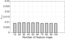
We observe first that increasing the depth of the network leads to a significant increase in the robustness to adversarial perturbations, especially from to layers. The depth of a neural network has an important impact on the robustness of the classifier, just like the degree of a polynomial classifier is an important factor for the robustness. Going from to layers however seems to have a marginal effect on the robustness. It should be noted that, despite the increase of the robustness with the depth, the normalized robustness computed for all classifiers is relatively small, which suggests that none of these classifiers is really robust to adversarial perturbations. Note also that the results in Figure 8 (a) showing an increase of the robustness with the depth are inline with recent results showing that depth provides robustness to adversarial geometric transformations (Fawzi and Frossard, 2015). In Fig. 8 (b), we show the effect of the number of feature maps in the CNN (for a one layer CNN) on the estimated normalized robustness to adversarial perturbations. Unlike the effect of depth, we observe that the number of feature maps has barely any effect on the robustness to adversarial perturbations. Finally, a comparison of the normalized robustness measures of very deep networks VGG-16 and VGG-19 (Simonyan and Zisserman, 2014) on ImageNet shows that these two networks behave very similarly in terms of robustness (both achieve a normalized robustness of ). This experiment, along with the experiment in Figure 8 (a), empirically suggest that adding layers on top of shallow network helps in terms of adversarial robustness, but if the depth of the network is already sufficiently large, then adding layers only moderately changes that robustness.

8 Discussion and perspectives
The existence of a general limit on the adversarial robustness of classifiers (established in Lemma 4.1) is an important phenomenon with many practical implications. To better understand the implications of this limit, we derived specialized upper bounds for two families of classifiers. For the family of linear classifiers, the established limit is very small for most problems of interest. Hence, linear classifiers are usually not robust to adversarial noise (even though robustness to random noise might be achieved). This is however different for nonlinear classifiers: for the family of quadratic classifiers, the limit on adversarial robustness is usually larger than for linear classifiers, which gives hope to have classifiers that are robust to adversarial perturbations. In fact, by using an appropriate training procedure, it might be possible to get closer to the theoretical bound. For general nonlinear classifiers (e.g., neural networks), designing training procedures that specifically take into account the robustness in the learning is an important future work. We also believe that the application of our general upper bound in Lemma 4.1 to derive explicit upper bounds that are specific to e.g., deep neural networks is an important future work. To do that, we believe that it is important to derive explicitly the parameters of assumption (A) for the class of functions under consideration. Results from algebraic geometry seem to suggest that establishing such results might be possible for general classes of functions (e.g., piecewise linear functions). In addition, experimental results suggest that, unlike the breadth of the neural network, the depth plays a crucial role in the adversarial robustness. Identifying an upper bound on the adversarial robustness of deep neural networks in terms of the depth of the network would be a great step towards having a better understanding of such systems.
Acknowledgments
We thank Hamza Fawzi, Ian Goodfellow for discussions and comments on an early draft of the paper, and Guillaume Aubrun for pointing out a reference for Theorem A.2. We also thank Seyed Mohsen Moosavi for his help in preparing experiments.
References
- Barreno et al (2006) Barreno M, Nelson B, Sears R, Joseph A, Tygar D (2006) Can machine learning be secure? In: ACM Symposium on Information, computer and communications security, pp 16–25
- Biggio et al (2012) Biggio B, Nelson B, Laskov P (2012) Poisoning attacks against support vector machines. In: International Conference on Machine Learning (ICML)
- Bousquet and Elisseeff (2002) Bousquet O, Elisseeff A (2002) Stability and generalization. The Journal of Machine Learning Research 2:499–526
- Caramanis et al (2012) Caramanis C, Mannor S, Xu H (2012) Robust optimization in machine learning. In: Sra S, Nowozin S, Wright SJ (eds) Optimization for machine learning, Mit Press, chap 14
- Chalupka et al (2014) Chalupka K, Perona P, Eberhardt F (2014) Visual causal feature learning. arXiv preprint arXiv:14122309
- Chang and Lin (2011) Chang CC, Lin CJ (2011) LIBSVM: A library for support vector machines. ACM Transactions on Intelligent Systems and Technology 2:27:1–27:27
- Chang et al (2010) Chang YW, Hsieh CJ, Chang KW, Ringgaard M, Lin CJ (2010) Training and testing low-degree polynomial data mappings via linear svm. The Journal of Machine Learning Research 11:1471–1490
- Dalvi et al (2004) Dalvi N, Domingos P, Sanghai S, Verma D (2004) Adversarial classification. In: ACM SIGKDD, pp 99–108
- Fan et al (2008) Fan RW, Chang KW, Hsieh CJ, Wang XR, Lin CJ (2008) Liblinear: A library for large linear classification. The Journal of Machine Learning Research 9:1871–1874
- Fawzi and Frossard (2015) Fawzi A, Frossard P (2015) Manitest: Are classifiers really invariant? In: British Machine Vision Conference (BMVC), pp 106.1–106.13
- Goldberg and Elhadad (2008) Goldberg Y, Elhadad M (2008) splitsvm: fast, space-efficient, non-heuristic, polynomial kernel computation for nlp applications. In: 46th Annual Meeting of the Association for Computational Linguistics on Human Language Technologies: Short Papers, pp 237–240
- Goodfellow (2015) Goodfellow I (2015) Adversarial examples, URL http://www.iro.umontreal.ca/~memisevr/dlss2015/goodfellow_adv.pdf, presentation at the Deep Learning Summer School, Montreal
- Goodfellow et al (2015) Goodfellow I, Shlens J, Szegedy C (2015) Explaining and harnessing adversarial examples. In: International Conference on Learning Representations
- Gu and Rigazio (2014) Gu S, Rigazio L (2014) Towards deep neural network architectures robust to adversarial examples. arXiv preprint arXiv:14125068
- Krizhevsky and Hinton (2009) Krizhevsky A, Hinton G (2009) Learning multiple layers of features from tiny images. Master’s thesis, Department of Computer Science, University of Toronto
- Lanckriet et al (2003) Lanckriet G, Ghaoui L, Bhattacharyya C, Jordan M (2003) A robust minimax approach to classification. The Journal of Machine Learning Research 3:555–582
- LeCun et al (1998) LeCun Y, Bottou L, Bengio Y, Haffner P (1998) Gradient-based learning applied to document recognition. Proceedings of the IEEE 86(11):2278–2324
- Lewis and Pang (1998) Lewis A, Pang J (1998) Error bounds for convex inequality systems. In: Generalized convexity, generalized monotonicity: recent results, Springer, pp 75–110
- Li et al (2014) Li G, Mordukhovich B, Phạm T (2014) New fractional error bounds for polynomial systems with applications to hölderian stability in optimization and spectral theory of tensors. Mathematical Programming pp 1–30
- Łojasiewicz (1961) Łojasiewicz S (1961) Sur le probleme de la division. to complete
- Lugosi and Pawlak (1994) Lugosi G, Pawlak M (1994) On the posterior-probability estimate of the error rate of nonparametric classification rules. IEEE Transactions on Information Theory 40(2):475–481
- Luo and Luo (1994) Luo X, Luo Z (1994) Extension of hoffman’s error bound to polynomial systems. SIAM Journal on Optimization 4(2):383–392
- Luo and Pang (1994) Luo ZQ, Pang JS (1994) Error bounds for analytic systems and their applications. Mathematical Programming 67(1-3):1–28
- Matoušek (2002) Matoušek J (2002) Lectures on discrete geometry, vol 108. Springer New York
- Moosavi-Dezfooli et al (2016) Moosavi-Dezfooli SM, Fawzi A, Frossard P (2016) Deepfool: a simple and accurate method to fool deep neural networks. In: IEEE Conference on Computer Vision and Pattern Recognition (CVPR)
- Ng and Zheng (2003) Ng K, Zheng X (2003) Error bounds of constrained quadratic functions and piecewise affine inequality systems. Journal of optimization theory and applications 118(3):601–618
- Nguyen et al (2014) Nguyen A, Yosinski J, Clune J (2014) Deep neural networks are easily fooled: High confidence predictions for unrecognizable images. arXiv preprint arXiv:14121897
- Pang (1997) Pang J (1997) Error bounds in mathematical programming. Mathematical Programming 79(1-3):299–332
- Simonyan and Zisserman (2014) Simonyan K, Zisserman A (2014) Very deep convolutional networks for large-scale image recognition. arXiv preprint arXiv:14091556
- Szegedy et al (2014) Szegedy C, Zaremba W, Sutskever I, Bruna J, Erhan D, Goodfellow I, Fergus R (2014) Intriguing properties of neural networks. In: International Conference on Learning Representations (ICLR)
- Xu et al (2009) Xu H, Caramanis C, Mannor S (2009) Robustness and regularization of support vector machines. The Journal of Machine Learning Research 10:1485–1510
Appendix A Proofs
A.1 Proof of Lemma 4.1
We begin by proving the following inequality:
Lemma A.1.
Let be non-negative real numbers, and let . Then,
Proof.
We prove that the quantity
is bounded from above by . To do so, let , and let us determine the maximum of the concave function . Setting the derivative of with respect to to zero, we get
hence . We therefore get , and conclude that the maximum of is reached when and the value of the maximum is . ∎
We now prove Lemma 4.1.
Proof.
The goal is to find an upper bound on .
Using assumption (A), the following upper bounds hold:
Hence, we obtain the following inequality on :
Using Jensen’s inequality, we have , for any random variable , and . Using this inequality together with , we obtain
We use the result in Lemma A.1 with , and obtain
Note moreover that the following equality holds
Using the above equality along with a similar one for , the following upper bound is obtained
which simplifies to
Observe moreover that , and that is bounded from above by . We therefore conclude that
∎
A.2 Proof of Theorem 5.3
The proof of this theorem relies on the concentration of measure on the sphere. The following result from (Matoušek, 2002) precisely bounds the measure of a spherical cap.
Theorem A.2.
Let denote the spherical cap of height . Then for , we have , and for , we have:
Based on Theorem A.2, we show the following result:
Lemma A.3.
Let be a vector of unit norm in . Let , and be a vector sampled uniformly at random from the unit sphere in . Then,
Proof.
Using an appropriate change of basis, we can assume that . For , we have
where (a) uses the upper bound of Theorem A.2, and (b) uses the inequality . Note moreover that for , the inequality holds, which proves the upper bound.
We now prove the lower bound. Observe that the following lower bound holds for , for any :
To see this, note that the maximum of the function is equal to . Therefore, , or equivalently, . Therefore, we get , and using Theorem A.2, we obtain for any :
Note also that this inequality holds for , as . ∎
Armed with the concentration of measure result on the sphere, we now focus on the proof of Theorem 5.3. Let . Let be fixed such that , and let and . Then,
Using the upper bound in Lemma A.3, we obtain:
Therefore, for , we obtain , and we deduce that
Using the lower bound result of Lemma A.3, we have:
This implies that for any , we have . Hence, we obtain the following upper bound on :
We also derive a lower bound on of the form by noting that
where we have used the fact that is a decreasing function of . To see that this function is indeed decreasing, note that its derivative (with respect to ) can be written as , with non-negative, and . Then, by using the inequality , the negativity of the derivative follows.
By combining the lower and upper bounds, and taking the expectations on both sides of the inequality, we obtain:
A similar result can be proven for such that . We therefore conclude that
where we have used the inequality .
Appendix B Vertical-horizontal example: quadratic classifier
We consider the quadratic classifier , with
We perform a change of basis, and work in the diagonalizing basis of , denoted by . We have
By letting , we have:
Given a point and label , the following problem is solved to find the minimal perturbation that switches the estimated label:
Let us consider the first datapoint (the other points can be handled in an exactly similar fashion). Then, it is easy to see that and , and the optimal point is achieved for and . In the original space, this point corresponds to . Therefore, , and we obtain .
Appendix C Discussion on the norms used to measure the magnitude of adversarial perturbations
The goal of this section is to discuss different ways of measuring the robustness to adversarial perturbations.
Given a datapoint , let be such that we know a priori that all points in the region
have the same true class as (i.e., a human observer would classify all images in this region similarly). Here defines a norm in the image space. Note that only depends on the dataset, but does not depend on any classifier . We defined the robustness of to adversarial perturbations, at , to be
The classifier is said to be not robust at if
| (15) |
In words, this means that there exists a point in the region (i.e., and are classified in the same way by a human observer), but is classified differently than by . Our main theoretical result provides upper bounds to (the expectation of ) in terms of interpretable quantities (i.e., distinguishability and risk): . Using this upper bound and Eq. (15), we certify that is not robust to adversarial perturbations when the following sufficient condition holds:
| (16) |
The main difficulty in the above definitions lies in the choice of and : how can be chosen to guarantee that contains all images of the same underlying class as ? In the original paper (Szegedy et al, 2014), is set to be the norm, but no is formally derived; classifiers are said to be not robust to adversarial perturbations when is judged to be “sufficiently small”. For example, it appears from Table 1 in (Szegedy et al, 2014) that if , the minimum required perturbation is thought to be small enough to guarantee that the images do not change their true underlying label. Motivated by the fact that pixels (or features) have limited precision, (Goodfellow et al, 2015) consider instead the norm, and ideally assume that a perturbation that have norm smaller than the precision of the pixels (e.g., 1/255 of the dynamic range for 8-bit images) is guaranteed to conserve the true underlying class. While this corresponds to setting to be the precision of the pixels, in practice it is set to be much larger for the MNIST case, as the images are essentially binary. In our case, the norm is considered, and we define the quantity to be the average norm of the minimal perturbation required to transform a training point to a training point of the opposite class:
We assume that the image is of the same underlying label as if is one order of magnitude smaller than . This corresponds to setting . A summary of the different choices is shown in Table 5.
| (Szegedy et al, 2014) | - | |
|---|---|---|
| (Goodfellow et al, 2015) | Determined by the image precision (in theory). Larger in practice. | |
| Ours |
All the above choices represent proxies of what we really would like to capture (i.e., the notion of perceptibility and class change). They all have some benefits and drawbacks, which we mention briefly now. We first acknowledge that the norm with blocks class changes (and therefore provides a sufficient condition for certifying the non-robustness of classifiers) for images that are essentially binary (e.g, MNIST digit images). In those cases, the norm seems more appropriate to use than the norm. However, in order to compare both norms, we need to carefully (and fairly) choose the parameter for both norms. In fact, if it is acknowledged that and provides a valid region where underlying image classes do not change, then and also provides a valid region, as for any vector . It is therefore all a matter of choosing a right threshold that is fair for all norms, if we wish to compare the norms for the task that we have at hand. A comparison between the and norm is provided in (Goodfellow, 2015), and it is concluded that, while the norm allows for class changes within its region, the essentially blocks the class changes and therefore constitutes a better choice. In more details, the comparison goes as follows: it is first argued that by choosing and , the region contains both a “natural” and , and therefore does not provide a valid region. To show the benefits of the norm, the author proceeds by considering and . It is then argued that this region blocks previous attempts for class changes, and therefore the norm provides a better choice for the task at hand. While this type of comparison is important in order to reach a better understanding of the norms used to measure the adversarial examples, it is not conclusive as it is unfair to the norm. Let us recall the following inequalities
| (17) |
For a fixed , define the regions:
It should be noted that for any , we have using Eq. (17). Not only that, but constitutes a tiny portion of in high dimensional spaces (i.e., the volume of over that of decays exponentially with the dimension). Therefore, a comparison of to will typically lead to problematic images in but not in , as is much bigger than . Therefore, the fact that is a much smaller set than (i.e., it contains much less images) is already known from Eq. (17) and is not conclusive in terms of the comparison of the two norms for measuring the robustness to adversarial perturbations. Just like the comparison of to is unfair to the norm, saying that the norm is better than the norm because contains much more images (potentially problematic ones with class changes, for sufficiently large ) that are not in is unfair to the norm.
One possible way for providing a fair comparison between both norms is to find the coefficient such that has the same volume as the following ball
Using mathematical derivations that we omit for the flow of this short discussion, we obtain asymptotically as . We argue that the comparison of to provides a more conclusive experiment than comparing to , as it highlights the advantage of one norm with respect to the other without biases on the volume of the region. In practice, this new comparison implies the following change for the “3” vs. “7” example in Goodfellow (2015): instead of allowing perturbations of max-norm , perturbations with norm up to are allowed. This will result in images that are roughly twice as much perturbed, for the case. Even with this comparison, it is possible that the max-norm in this case will also block attempts to change the class, as the images are essentially binary. We believe that the is probably a better choice in this case.


However, this is not a general statement, as in some cases of non-binary images, the norm might be a better choice. We illustrate the above statement on a toy example where the goal is to classify sport balls. Some example images are shown in Fig. 9. In this example, the norm between any two images is less than . Setting with does not define a valid region (i.e., it does not guarantee that no class changes will occur within the region). On the other hand, the region computed with (i.e., ) rightfully excludes the images b) and c) from the space of valid perturbations of a). This toy example provides a proof of concept that shows that, in some cases, the norm might actually be a better choice than the norm.
In conclusion, we stress that this example has no intention of proving that the norm is universally better than the norm to measure the norm of adversarial perturbations. Through this discussion and example, we show that there is no universal answer to which norm one has to use to measure the robustness to adversarial perturbations, as it is strongly application-dependent. We believe more theoretical research in that area is needed in order to fully grasp the advantage of each norm, and probably design new norms that are suitable for measuring adversarial perturbations.