From Rubber Bands to Rational Maps:
A Research Report

Abstract.

This research report outlines work, partially joint with Jeremy Kahn and Kevin Pilgrim, which gives parallel theories of elastic graphs and conformal surfaces with boundary. On one hand, this lets us tell when one rubber band network is looser than another and, on the other hand, tell when one conformal surface embeds in another.

We apply this to give a new characterization of hyperbolic critically finite rational maps among branched self-coverings of the sphere, by a positive criterion: a branched covering is equivalent to a hyperbolic rational map if and only if there is an elastic graph with a particular “self-embedding” property. This complements the earlier negative criterion of W. Thurston.

1. Introduction

This research report is devoted to explaining a circle of ideas, relating:

• elastic networks (“rubber bands”) and the corresponding Dirichlet energy,

• extremal length and other “quadratic” norms on the space of curves in a surface,

• embeddings between Riemann surfaces, conformal or quasi-conformal, and

• post-critically finite rational maps.

The original motivation for this project is the last point, and more specifically the question of when a topological branched self-covering of the sphere is equivalent to a rational map. William Thurston first answered this question more than 30 years ago [DH93:ThurstonChar], by giving a “negative” characterization: a combinatorial obstruction that exists exactly when the map is not rational (Theorem LABEL:thm:thurston-obstruction). In this paper, we give a “positive” characterization: a combinatorial object that exists exactly when the map is rational, for a somewhat restricted class of maps (Theorem 1).

Having both positive and negative combinatorial characterizations for the same property automatically gives an algorithm for testing the property. You search, in parallel, for either an obstruction or a certificate for the property. One of the searches will eventually succeed and answer the question. There are other algorithms for testing whether a branched self-cover is rational: you may take the rational map itself as a certificate for being rational [BBY12:RatlMapDecidable]. However, we expect our combinatorial certificate to be more practical to search for (Section 6.6). By contrast, W. Thurston’s obstruction theorem is notoriously hard to apply.

In addition, a positive characterization gives an object to study associated to the topological branched self-covers of most interest, namely the rational ones.

Several of the constructions along the way are of independent interest. For instance, we give a new characterization of when one Riemann surface conformally embeds in another in a given homotopy class, and a numerical invariant of such embeddings.

This is a preliminary report on the results. Most proofs are omitted, although we give some indications. We also indicate some of the many open problems suggested by this research in the subsections titled “Extensions” (Sects. 3.4, 5.5, 6.7, 7.4, and LABEL:sec:rational-extensions); all of these are unnecessary for the main results.

1.1. Detecting rational maps

Recall that a (topological) branched self-cover of the sphere is a finite set of points $P$ in the sphere and a map $f:(S^{2},P)\to(S^{2},P)$ that is a covering when restricted to $S^{2}\setminus f^{-1}(P)$. One central question is when such a map is equivalent to a rational map on $\mathbb{C}\mathbb{P}^{1}$. (See Definition 8.1.) A branched self-cover can be characterized (up to homotopy) by picking a spine $\Gamma$ for $S^{2}\setminus P$, and drawing its inverse image $\widetilde{\Gamma}=f^{-1}(\Gamma)\subset S^{2}\setminus f^{-1}(P)$. There are two natural homotopy classes of maps from $\widetilde{\Gamma}$ to $\Gamma$. (In this paper, a map of graphs is a topological map, not necessarily taking vertices to vertices.)

• A covering map commuting with the action of $f$:

  We denote this covering map $\pi:\widetilde{\Gamma}\to\Gamma$.

• A map commuting up to homotopy with the inclusion in $S^{2}\setminus P$:

  We denote this map $\phi$. It is unique up to homotopy since $\Gamma$ is a spine for $S^{2}\setminus P$.

$\Gamma=\,\,\,\,\vbox{\hbox{$\includegraphics[trim=-1.00374pt -1.00374pt -1.00374pt -1.00374pt]{graphs-11}$}}$ $\widetilde{\Gamma}=\,\,\,\,\vbox{\hbox{$\includegraphics[trim=-1.00374pt -1.00374pt -1.00374pt -1.00374pt]{graphs-12}$}}$

Figure 1. A spine and its inverse image defining a branched self-cover of the sphere. The marked set $P$ consists of the two points shown, and a third point $C$ at infinity. The numbers on the edges give a measure which proves this branched self-cover is equivalent to a rational map.

Example 1.1.

Figure 1 shows a simple example of such spines when $P$ has 3 points, $A$, $B$, and $C$ (at $\infty$). The covering map $\pi$ preserves the colors and arrows on the edges. The branched self-cover $f:(S^{2},P)\righttoleftarrow$ is an extension of $\pi$ to the whole sphere. This extension is unique up to homotopy relative to $\{A,B,C\}$. The map $f$ permutes the marked points by

(For instance, $A$ is inside a crimson-goldenrod region in $\widetilde{\Gamma}$, so must map to $B$, which is inside a crimson-goldenrod region in $\Gamma$.)

The map $\phi$, on the other hand, is the projection of $\widetilde{\Gamma}$ onto $\Gamma$ considered as a spine; for instance, it might map the right-hand purple edge of $\widetilde{\Gamma}$ to the right-hand goldenrod edge of $\Gamma$, whereas $\pi$ preserves the colors.

For our characterization of rational maps, we also need an elastic structure on $\Gamma$, by which we mean a measure $\alpha$ on $\Gamma$ absolutely continuous with respect to Lebesgue measure. We can pull back $\alpha$ by $\pi$ to get a measure $\pi^{*}\alpha=\widetilde{\alpha}$ on $\widetilde{\Gamma}$. For $\psi:\widetilde{\Gamma}\to\Gamma$ a Lipschitz map of graphs, define the embedding energy by

(1.1) $$\operatorname{Emb}(\psi)\coloneqq\operatorname*{ess\,sup}_{y\in\Gamma}\sum_{\begin{subarray}{c}x\in\widetilde{\Gamma}\\ \psi(x)=y\end{subarray}}\lvert\psi^{\prime}(x)\rvert.$$

The derivative is taken with respect to the two measures $\widetilde{\alpha}$ and $\alpha$. The essential supremum $\operatorname*{ess\,sup}$ ignores points of measure zero. In particular, we may ignore vertices of $\widetilde{\Gamma}$ or points of $\widetilde{\Gamma}$ that map to vertices of $\Gamma$.

In practice the embedding energy is optimized when $\psi$ is piecewise linear, and the reader may restrict to that case.

For one motivation for Equation (1.1), see Proposition 6.23: the embedding energy characterizes conformal embeddings of thickened versions of the graph. Another one is in Theorem 6: it characterizes when Dirichlet energy is reduced under the map, i.e., when one rubber band network is looser than another. (See Remark 6.19.)

Example 1.2.

To return to Example 1.1, consider the measure $\alpha$ on $\Gamma$ from Figure 1 and the concrete map $\psi:\widetilde{\Gamma}\to\Gamma$ that maps

• the right purple edge of $\widetilde{\Gamma}$ to the goldenrod edge on the right of $\Gamma$,

• the right goldenrod edge of $\widetilde{\Gamma}$ to the crimson edge in the middle of $\Gamma$, and

• the remaining four edges (two crimson, one goldenrod, and one purple) of $\widetilde{\Gamma}$ map to the purple edge on the right of $\Gamma$, with the crimson edges mapping to segments of length $1/\sqrt{2}$.

Make $\psi$ linear on each segment described above. Then a short computation shows that $\operatorname{Emb}(\psi)=1/\sqrt{2}$.

A major theorem of this paper is that rational maps can be characterized by maps $\psi$ with embedding energy less than $1$. We say that two branched self-covers $f_{1}:(S^{2},P_{1})\righttoleftarrow$ and $f_{2}:(S^{2},P_{2})\righttoleftarrow$ are equivalent if they can be connected by a homotopy of $f_{1}$ relative to $P_{1}$ and conjugacy taking $P_{1}$ to $P_{2}$.

Theorem 1.

Let $f:(S^{2},P)\righttoleftarrow$ be a branched self-cover of the sphere. Suppose that there is a branch point in each cycle in $P$. Then $f$ is equivalent to a rational map iff there is an elastic graph spine $(\Gamma,\alpha)$ for $S^{2}\setminus P$, an integer $n>0$, and map $\psi\in[\phi_{n}]$ so that $\operatorname{Emb}(\psi)<1$.

Here $\phi_{n}$ is obtained from $\phi$ by iteration, and is in the homotopy class of the projection $f^{-n}(\Gamma)\to\Gamma$. Loosely speaking, Theorem 1 says that the self-cover is rational iff there is a self-embedded spine for $S^{2}\setminus P$.

Remark 1.3.

It is likely the condition on Theorem 1 can be relaxed to assume merely that $f$ has at least one branch point in one cycle in $P$, i.e., if $f$ is rational, its Julia set is not the whole sphere. See Section LABEL:sec:rational-extensions.

Example 1.4.

The explicit measure and map in Example 1.2 show that the given branched self-cover is equivalent to a rational map. In fact, it is equivalent to the rational map

$$f(z)=\frac{1}{1-z^{2}},$$

with $A=0$, $B=1$, and $C=\infty$.

There was a previous characterization of rational maps by W. Thurston, recalled as Theorem LABEL:thm:thurston-obstruction below. This is analogous to the two ways to characterize pseudo-Anosov surface automorphisms, which form a natural class of geometric elements of the mapping class group of a surface. Geometrically, pseudo-Anosov diffeomorphisms are those whose mapping torus is a hyperbolic 3-manifold. Combinatorially, there are two criteria:

• Negative: $f$ is pseudo-Anosov iff it is not periodic ($f^{\circ k}$ is not the identity for any $k>0$) or reducible (there is no invariant system of multi-curves for $f$).

• Positive: $f$ is pseudo-Anosov iff there is a measured train track $T$ and a splitting sequence from $T$ to a train-track $T^{\prime}$ with $T^{\prime}=\lambda f(T)$ for some constant $0<\lambda<1$ [PP87:CharPAnosov].

The positive criterion gives some extra information: the number $\lambda$ is an invariant of $f$, with dynamical interpretations. (For instance, $\lambda$ controls the growth rate of intersection numbers.)

Analogously, we can say that a branched self-cover $f$ of $(S^{2},P)$ is geometric if it is equivalent to a rational map, which also have associated 3-dimensional hyperbolic laminations [LM97:LaminationsHolomorphic]. There are combinatorial criteria for $f$ to be rational:

• Negative: $f$ is rational iff there is no obstruction, as in W. Thurston’s Theorem LABEL:thm:thurston-obstruction. In loose terms, the obstruction is a back-expanding annular system: a collection of annuli that get “wider” under backwards iteration.

• Positive: Under some additional assumptions, $f$ is rational iff there is a metric spine for $S^{2}\setminus P$ satisfying a back-contracting condition. This is Theorem 1.

As in the case of surface automorphisms, the two theorems are in a sense “dual” to each other: it is easy to see that a branched-self cover cannot simultaneously have a back-expanding annular system and a back-contracting spine. (See Equation (LABEL:eq:obstruction-cd).) Also as in the surface automorphism case, the positive criterion gives us a new object to study, namely the constant $\overline{\operatorname{SF}}[\phi]$ of Section 7.2.

Compared to the situation for surface automorphisms, Theorem 1 has the following caveats:

• It only works when there is a branch point in each cycle in $P$. (But see Remark 1.3.)

• We may need to pass to an iterate to get $\operatorname{Emb}(\phi)<1$. Furthermore, it is easy to see in examples that the embedding energy can decrease in powers. (In the notation of Section 7.2, in general $\operatorname{SF}[\phi_{n}]<\operatorname{SF}[\phi]^{n}$ and $\overline{\operatorname{SF}}[\phi]<\operatorname{SF}[\phi]$. See Example 2.7.)

There is a further caveat for both surface automorphisms and branched self-covers:

• For the positive criterion, the train track or graph constructed is not canonical: there are many different choices that work for the criterion.

By contrast, the negative criteria can be made canonical. (Pilgrim [Pilgrim01:CanonicalObstruction] proved this for branched self-covers.) On the other hand, in the surface case, Agol [Agol11:pAtriangulation] and Hamenstädt [Hamenstaedt09:GeomMCG1] give a canonical object related to the measured train track.

1.2. Elastic graphs

The embedding energy of Equation (1.1) looks a little mysterious; it looks a little like the Lipschitz stretch factor, but the sum over inverse images looks unusual. To explain where it comes from, we now turn to a “conformal” theory of graphs parallel to the conformal theory of Riemann surfaces. The central object is an elastic graph $(\Gamma,\alpha)$, which you should think of as a network of rubber bands; formally, it is a graph with a measure on each edge, representing the elasticity of the edge. (See Section 3.3.)

There are additional structures we can put on the graph.

• On one hand, we can consider curves $C$ on the graph, maps from a 1-manifold into $\Gamma$.

• On the other hand, we can consider maps from $\Gamma$ to a length graph $K$, a graph with fixed lengths of edges (like a network of pipes).

Maps between these objects have naturally associated energies, as summarized in the following diagram.

(1.2)

The labels on the arrows indicate the type of energy on a map of this type, as follows.

• For a map $f$ from an elastic graph $(\Gamma,\alpha)$ to a length graph $(K,\ell)$, there is the Dirichlet or rubber-band energy (Section 4) familiar from physics:

  (1.3) $$\operatorname{Dir}(f)\coloneqq\int_{x\in\Gamma}\lvert f^{\prime}(x)\rvert^{2}\,dx,$$

  where $f^{\prime}$ measures the derivative with respect to the natural metrics. If $f$ minimizes this energy within its homotopy class, it is said to be harmonic.

• For a curve $C$ in an elastic graph $(\Gamma,\alpha)$, we have a version of extremal length (Section 5):

  (1.4) $$\operatorname{EL}[C]\coloneqq\sum_{e\in\operatorname{Edge}(\Gamma)}n_{C}(e)^{2}\cdot\alpha(e),$$

  where $n_{C}(e)$ is the number of times $C$ runs over the edge $e$ (without backtracking).

• For a curve $C$ in a length graph $(K,\ell)$, we have the usual length, which in our notation is

  (1.5) $$\ell[C]\coloneqq\sum_{e\in\operatorname{Edge}(K)}n_{C}(e)\cdot\ell(e).$$

  To match the other quantities, we actually use the square of the length as our energy.

• For a map $\phi$ between length graphs $(K_{1},\ell_{1})$ and $(K_{2},\ell_{2})$, there is the Lipschitz constant (Section 4.3):

  (1.6) $$\operatorname{Lip}(\phi)\coloneqq\operatorname*{ess\,sup}_{x\in K_{1}}\lvert\phi^{\prime}(x)\rvert.$$

  Again, we consider the square of the Lipschitz energy.

• Finally, for a map $\phi$ between elastic graphs $(\Gamma_{1},\alpha_{1})$ and $(\Gamma_{2},\alpha_{2})$, we have embedding energy as used in Theorem 1 (Section 6):

  (1.7) $$\operatorname{Emb}(\phi)\coloneqq\operatorname*{ess\,sup}_{y\in\Gamma_{2}}\sum_{x\in\phi^{-1}(y)}\lvert\phi^{\prime}(x)\rvert.$$

  This energy appears to be new, although it is related to Jeremy Kahn’s notion of domination of weighted arc diagrams (Section LABEL:sec:dynam-teich).

Remark 1.5.

We could make the diagram more symmetric by using width graphs instead of curves (see Section 3.3), and adding a norm on maps between width graphs.

These energies are sub-multiplicative, in the sense that composing two maps can only decrease the product of the energies: if $f$ and $g$ are two composable maps of the above types, then

(1.8) $$\lVert f\circ g\rVert\leq\lVert f\rVert\cdot\lVert g\rVert,$$

where $\lVert\cdot\rVert$ is the appropriate energy from the above list. (This inequality is the reason we squared some of the energies.) For instance, if we fix elastic graphs $\Gamma_{1}$ and $\Gamma_{2}$, a length graph $K$, and maps $\phi:\Gamma_{1}\to\Gamma_{2}$ and $f:\Gamma_{2}\to K$, then

(1.9) $$\operatorname{Dir}(f\circ\phi)\leq\operatorname{Dir}(f)\cdot\operatorname{Emb}(\phi)$$

What is more, these inequalities are all tight, in the sense that if we fix the domain, range, and homotopy type of $f$, then we can find a sequence of functions $g_{i}$ (including a choice of domain) that approach equality in Equation (1.8). Likewise if we fix $g$ and vary $f$, we can find a sequence of functions $f_{i}$ approaching equality in Equation (1.8).

For instance, if $\phi:\Gamma_{1}\to\Gamma_{2}$ is a map of elastic graphs, we can strengthen Equation (1.9) to

(1.10) $$\operatorname{Emb}[\phi]=\sup_{\begin{subarray}{c}\text{$K$ length graph}\\ f:\Gamma_{2}\to K\end{subarray}}\frac{\operatorname{Dir}[f\circ\phi]}{\operatorname{Dir}[f]},$$

where $\operatorname{Emb}[\phi]$ and $\operatorname{Dir}[f]$ are the minimums over the respective homotopy classes (Theorem 6). Since Dirichlet energy can be interpreted as the elastic energy of a stretched rubber band network, $\operatorname{Emb}[\phi]<1$ can therefore also be interpreted as saying that $\Gamma_{1}$ is “looser” than $\Gamma_{2}$, however the two rubber band networks are stretched. See Remark 6.19.

Other examples are in Propositions 5.13 and 5.14. This gives a kind of duality between curves in an elastic graph $\Gamma$ and maps from $\Gamma$ to length graphs. If we think of curves as living in a “vector space” and maps to length graphs in its “dual”, then the embedding energy can be interpreted as an “operator norm”.

This theory of conformal graphs is largely parallel to the theory of conformal (Riemann) surfaces with boundary, where we again have a number of energies:

(1.11)

Again, each arrow is marked by the appropriate energy for measuring that type of map. $\operatorname{Dir}$ and $\operatorname{EL}$ are again Dirichlet energy and extremal length, but on surfaces rather than graphs. $\operatorname{SF}$ is new; it is the stretch factor of a homotopy class of a topological embedding $[\phi]:\Sigma_{1}\to\Sigma_{2}$ between Riemann surfaces. In general, we do not know a direct expression analogous to Equation (1.1), so $\operatorname{SF}$ is defined to be the minimal ratio of extremal lengths (Definition 6.2, analogous to Equation (1.10)). When there is no conformal embedding of $\Sigma_{1}$ in $\Sigma_{2}$ in the given homotopy class, there is a direct expression: $\operatorname{SF}[\phi]$ is given by the minimal quasi-conformal constant in the homotopy class (Theorem 3). There is an analogue of $\operatorname{SF}$ for maps between elastic graphs, and in that context $\operatorname{SF}[\phi]=\operatorname{Emb}[\phi]$ (Theorem 6).

Remark 1.6.

To prove Theorem 1, we actually do not need to consider length graphs or the Dirichlet energy at all. (The proofs go through extremal length instead.) However, they illuminate the overall structure. In particular, it is not clear why one would consider elastic graphs without the rubber-band motivation.

Remark 1.7.

The appearance of length squared in (1.2) and (1.11) is easy to justify on the grounds of units. Extremal length itself behaves like the square of a length, in the sense that if we take $k$ parallel copies of a curve, the extremal length multiplies by $k^{2}$. Likewise, if the lengths on the target of a harmonic map are multiplied by $k$, the harmonic map remains harmonic while the Dirichlet energy is multiplied by $k^{2}$.

1.3. History and prior work

Although Equation (1.1) appears to be new, Jeremy Kahn’s notion of domination of weighted arc diagrams [Kahn06:BoundsI] is essentially equivalent. See Section LABEL:sec:dynam-teich.

There has also been substantial work in the related setting of resistor networks rather than spring networks [BSST40:DissectionRects, Duffin62:ELNetwork, CIM98:CircNetworks, inter alia]. See Remark 4.4.

Theorem 1 is closely related to Theorem 8.4, which characterizes when a rational map exists in terms of conformal embeddings of surfaces. Theorem 8.4 has been a folk theorem in the community for some time.

For polynomials, Theorem 1 reduces to a previously-known characterization in terms of expansion on the Hubbard tree; see Theorem LABEL:thm:realize-hubbard in Section LABEL:sec:polynomials.

1.4. Organization

After a section giving some examples of how to apply Theorem 1, this paper is organized by topics moving up a dynamical hierarchy. For each topic we give first the conformal surface notions and then the graph notions.

• We start with notions depending only on a single conformal surface or graph: Dirichlet (or rubber band) energy of (harmonic) maps (Section 4) and extremal length of curves (Section 5).

• Next come notions depending on a map between surfaces or graphs. This is the stretch factor or embedding energy, which generalizes the Teichmüller distance and characterizes conformal embeddings of surfaces (Section 6).

• Next is the dynamical theory of iterated maps (Section 7). Here we find another number, the asymptotic stretch factor, which characterizes rational maps (Section 8).

The paper is organized by a logical hierarchy, rather than what is necessarily pedagogically best; the reader is encouraged to skip around.

1.5. Acknowledgements

I would like to thank Matt Bainbridge, Steven Gortler, Richard Kenyon, Sarah Koch, Tan Lei, Dan Margalit, and Giulio Tiozzo for many helpful conversations. I would like to especially thank Maxime Fortier Bourque, who pointed me towards Ioffe’s theorem [Ioffe75:QCImbedding] and had numerous other insights.

This project grew out of extensive conversations with Kevin Pilgrim, who helped shape my understanding of the subject in many ways. Many of the arguments were developed jointly with him. Notably, he communicated Theorem 8.4 to me, and Theorem 4 is joint work with him. Theorem 5 is joint work with Jeremy Kahn, who also contributed substantially throughout.

Above all, I would like to thank William Thurston for introducing me to the subject and insisting on understanding deeply.

2. Examples

Here, we give some more substantial examples of Theorem 1.

2.1. Polynomials: The rabbit and the basilica

Theorem 1 is not very interesting for polynomials, as every topological polynomial with a branch-point in each cycle is equivalent to a polynomial. The extension of Theorem 1 to the general topological polynomial case is somewhat more interesting, but is equivalent to known results on expansion on the Hubbard tree; see Section LABEL:sec:polynomials. Nevertheless, we will look at some examples, both to see what the stretch factors are and to use them for matings.

Example 2.1.

We first look at the “rabbit” polynomial, the post-critically finite polynomial $f_{1}(z)=z^{2}+c$ with $c\approx-0.1226+0.7449i$. The critical point moves in a 3-cycle

$$\vbox{\hbox{$\leavevmode\hbox to65.97pt{\vbox to51.77pt{\text{[drawing]}}}$}}. 0 c c^{2}+c \scriptstyle{(2)} 0 c c^{2}+c \scriptstyle{(2)}$$

The optimal elastic graph $\Gamma_{1}$ and its cover $\widetilde{\Gamma}_{1}$ are

$$\vbox{\hbox{$\includegraphics[trim=-1.00374pt -1.00374pt -1.00374pt -1.00374pt]{matings-51}$}}\longrightarrow\;\;\vbox{\hbox{$\includegraphics[trim=-1.00374pt -1.00374pt -1.00374pt -1.00374pt]{matings-50}$}},$$

with $\operatorname{Emb}[\widetilde{\Gamma}_{1}\to\Gamma_{1}]=2^{-1/3}$, which is less than one, as expected. (There is another marked point at infinity, not shown.)

Example 2.2.

Another graph $\Gamma_{2}$ that works to prove that the rabbit polynomial is realizable is

(2.1) $$\vbox{\hbox{$\includegraphics[trim=-1.00374pt -1.00374pt -1.00374pt -1.00374pt]{matings-2}$}}\;\;\longrightarrow\;\;\vbox{\hbox{$\includegraphics[trim=-1.00374pt -1.00374pt -1.00374pt -1.00374pt]{matings-1}$}}.$$

The black edges have the indicated lengths, which come from looking at the external rays landing at the $\alpha$ fixed point of $f_{1}$. Give the colored edges an equal and long elastic length (say, 100). There is a natural map $\phi_{0}:\widetilde{\Gamma}_{2}\to\Gamma_{2}$ as follows.

• The outside circle is mapped to the outside circle, with derivative $\lvert\phi_{0}^{\prime}\rvert=1/2$.

• The colored segments on the lower right of $\widetilde{\Gamma}_{2}$ is squashed out to the lower-right boundary of $\Gamma_{2}$, with derivative $\lvert\phi_{0}^{\prime}\rvert$ on order of $1/100$. Thus $\operatorname{Fill}_{\phi_{0}}\approx 1/2$ on the corresponding portion of $\Gamma_{2}$. ($\operatorname{Fill}_{\phi}$ is defined in Equation (4.4), and is the quantity maximized in the definition of $\operatorname{Emb}(\phi)$.)

• The colored segments in the upper left of $\widetilde{\Gamma}_{2}$ are mapped to the colored segments in $\Gamma_{2}$, with $\lvert\phi_{0}^{\prime}\rvert=1$.

Because of the last point, this map has $\operatorname{Emb}[\phi_{0}]=1$, which is not good enough. Let $\phi_{1}$ be the result of “pulling in” very slightly the image of the ends of the upper-left colored segments of $\widetilde{\Gamma}_{2}$, so they map to the interior of the colored segments of $\Gamma_{2}$. This decreases the derivative on the colored segments to less than one, while only increasing the derivative on the outside circle slightly; thus $\operatorname{Emb}[\phi_{1}]$ is very slightly less than $1$, as desired.

Example 2.3.

We can perform a similar trick for other polynomials. For instance, the basilica polynomial $f_{3}(z)=z^{2}-1$ has a spine $\Gamma_{3}$, with cover given by

(2.2) $$\vbox{\hbox{$\includegraphics[trim=-1.00374pt -1.00374pt -1.00374pt -1.00374pt]{matings-11}$}}\longrightarrow\vbox{\hbox{$\includegraphics[trim=-1.00374pt -1.00374pt -1.00374pt -1.00374pt]{matings-10}$}}.$$

The same argument as above (giving the purple edge a long length, and pushing the right purple edge out to the boundary) shows that there is a map $\phi:\widetilde{\Gamma}_{3}\to\Gamma_{3}$ with $\operatorname{Emb}[\phi]<1$. (In this case the optimal stretch factor is $2^{-1/2}$ and is not realized with a graph with this topology).

2.2. Matings

We can use the techniques of Section 2.1 to show that some matings of polynomials are geometrically realizable.

Example 2.4.

We can glue together the figures in Equations (2.1) and (2.2):

(2.3) $$\vbox{\hbox{$\includegraphics[trim=-1.00374pt -1.00374pt -1.00374pt -1.00374pt]{matings-21}$}}\longrightarrow\vbox{\hbox{$\includegraphics[trim=-1.00374pt -1.00374pt -1.00374pt -1.00374pt]{matings-20}$}}.$$

This gives a graph spine $\Gamma_{4}$ and cover $\widetilde{\Gamma}_{4}$ representing the formal mating of the rabbit and the basilica. We can find a map $\phi:\widetilde{\Gamma}_{4}\to\Gamma_{4}$ with embedding energy less than $1$:

• Assign the black mating circle in $\Gamma_{4}$ total length $1$, divided according to the angles of the external rays.

• Give all colored edges an equal and large length.

• Pull this metric back to $\widetilde{\Gamma}_{4}$, and map $\widetilde{\Gamma}_{4}$ to $\Gamma_{4}$ by pushing colored arcs out to the black circle as in Examples 2.2 and 2.3.

• Pull the map in slightly where colored vertices meet the black circle.

The result has $\operatorname{Fill}_{\phi}(y)$ slightly larger than $1/2$ when $y$ is on the black circle, and $\operatorname{Fill}_{\phi}(y)$ slightly less than one on the colored edges.

Naturally, the technique of Example 2.4 cannot always work, as sometimes the mating is not geometrically realizable.

Example 2.5.

If we try to mate a basilica with a basilica, we get these graphs:

(2.4) $$\vbox{\hbox{$\includegraphics[trim=-1.00374pt -1.00374pt -1.00374pt -1.00374pt]{matings-31}$}}\longrightarrow\vbox{\hbox{$\includegraphics[trim=-1.00374pt -1.00374pt -1.00374pt -1.00374pt]{matings-30}$}}.$$

If we try to use the same technique as before, it doesn’t work, as there are two points on the black circle that we attempt to pull in two different directions. Indeed, the left green-purple circle is mapped to a green-purple circle, so must have derivative at least $1$: it is an obstruction to the mating. (In this case, it is a Levy cycle).

2.3. Slit maps

Given a branched self-cover $f:(S^{2},P)\righttoleftarrow$ and an arc $A$ with endpoints in $P$, there is a blowing up construction which produces a map $f_{A}$ that agrees with $f$ outside of a neighborhood of $A$ and maps that neighborhood surjectively on to $S^{2}$. Pilgrim and Tan Lei showed that, if $f$ is a rational map, these blow ups frequently are as well [PT98:Combining]. We will restrict attention to cases where the initial map $f$ is the identity, in which case the theorem becomes the following.

Theorem 2.6.

Let $P\subset S^{2}$ be a finite graph, and let $G\subset S^{2}$ be a finite embedded graph with endpoints on $P$. Then $\mathrm{id}_{G}$ is a rational map iff $G$ is connected.

We can give a new proof in the harder direction, when $G$ is connected. We start with a simple example. From the connected planar graph

$$G=\vbox{\hbox{$\includegraphics[trim=-1.00374pt -1.00374pt -1.00374pt -1.00374pt]{graphs-40}$}},$$

take as spine $\Gamma_{4}$ the spherical dual to $G$. Then $\widetilde{\Gamma}_{4}$ is obtained by taking the connect sum of $\Gamma_{4}$ with four extra copies $\Gamma_{4}^{i}$ of $\Gamma_{4}$, one for each edge:

$$\vbox{\hbox{$\includegraphics[trim=-1.00374pt -1.00374pt -1.00374pt -1.00374pt]{graphs-42}$}}\longrightarrow\vbox{\hbox{$\includegraphics[trim=-1.00374pt -1.00374pt -1.00374pt -1.00374pt]{graphs-41}$}}.$$

For any metric on $\Gamma_{4}$, there is a natural map $\phi:\widetilde{\Gamma}_{4}\to\Gamma_{4}$ that maps most of each copy $\Gamma_{4}^{i}$ to a point in the center of the corresponding edge of $\Gamma_{0}$. This map $\phi$ has derivative equal to $1/2$ or $0$ everywhere. We have $\operatorname{Emb}(\phi)=1/2$, and consideration of the red edge shows that this is optimal.

This example generalizes immediately to a general connected graph $G$, except that $\operatorname{Emb}[\phi]$ will only be $1/2$ when $G$ has a univalent vertex; otherwise, $\operatorname{Emb}[\phi]$ will be strictly smaller. We have thus proved Theorem 2.6, with some additional information about the stretch factor.

2.4. Behavior under iteration

We can iterate Example 1.1:

$$\cdots\rightarrow\vbox{\hbox{$\includegraphics[trim=-1.00374pt -1.00374pt -1.00374pt -1.00374pt]{graphs-3}$}}\rightarrow\vbox{\hbox{$\includegraphics[trim=-1.00374pt -1.00374pt -1.00374pt -1.00374pt]{graphs-2}$}}\rightarrow\vbox{\hbox{$\includegraphics[trim=-1.00374pt -1.00374pt -1.00374pt -1.00374pt]{graphs-1}$}}$$

(See Section 7.1 for details on iteration.) In this example, the embedding energy behaves well, in the sense that the $k$’th iterate $\phi_{k}$ is optimal for embedding energy (using the edge lengths and concrete initial map from Example 1.2):

$$\operatorname{Emb}[\phi_{k}]=\operatorname{Emb}(\phi_{k})=\bigl{(}\sqrt{2}\bigr{)}^{-k}.$$

Such good behavior is not generally the case.

Example 2.7.

The map

$$f(z)=\frac{1+z^{2}}{1-z^{2}}$$

is represented combinatorially by a graph $\Gamma_{5}$ and maps $\pi,\phi:\widetilde{\Gamma}_{5}\rightrightarrows\Gamma_{5}$:

(2.5) $$\vbox{\hbox{$\includegraphics[trim=-1.00374pt -1.00374pt -1.00374pt -1.00374pt]{graphs-5}$}}\longrightarrow\vbox{\hbox{$\includegraphics[trim=-1.00374pt -1.00374pt -1.00374pt -1.00374pt]{graphs-1}$}}.$$

A case analysis shows that for any metric on $\Gamma$ and any map $\psi\in[\phi]$ with $\operatorname{Emb}(\psi)<1$, there is some power $1\leq k\leq 4$ so that the $k$-fold iterate $\psi_{k}$ has local back-tracking. This implies that

$$\operatorname{Emb}[\psi_{4}]<\operatorname{Emb}[\psi]^{4},$$

regardless of the initial metric. Similar facts hold for any of the other three graphs homotopy equivalent to $\Gamma_{5}$. Thus, regardless of the choice of initial spine, we have $\overline{\operatorname{SF}}[\phi]<\operatorname{SF}[\phi]=\operatorname{Emb}[\phi]$. (See Section 7.2 for definitions.)

Figure 2 gives a sample of experimental data for this map. An ad hoc argument shows that for this map, $\overline{\operatorname{SF}}[\phi]=2^{-1/3}$. The corresponding line is shown dashed in the figure.

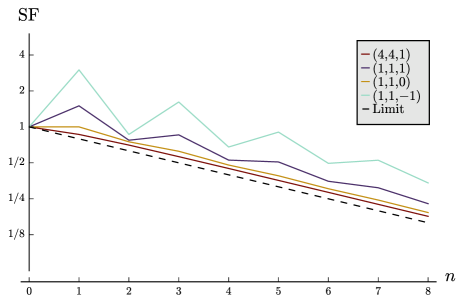
Figure 2. Logarithmic plot of $\operatorname{SF}[\phi_{n}]$ for $\phi$ from Example 2.7, as $n$ varies. The parameters $(\alpha,\beta,\gamma)$ are the elastic lengths of the left, right, and middle edges in Equation (2.5), respectively. When $\gamma=0$, the graph $\Gamma_{5}$ degenerates to a rose graph. The line for $(\alpha,\beta,\gamma)=(1,1,-1)$ corresponds instead to a barbell graph homotopy equivalent to $\Gamma_{5}$. The dashed line shows $\overline{\operatorname{SF}}[\phi]^{n}$.

3. Setting

3.1. Surfaces

We work with compact, oriented surfaces $\Sigma$ with boundary. It is sometimes convenient to think about the double $D\Sigma=\Sigma\cup_{\partial}\overline{\Sigma}$, which has no boundary.

Definition 3.1.

A curve on $\Sigma$ is an immersion of a 1-manifold with boundary in $\Sigma$, with boundary mapped to the boundary. The 1-manifold need not be connected; if it is, the curve is said to be connected. Curves are considered up to homotopy within the space of all maps taking the boundary to the boundary (not necessarily immersions). A curve is simple if it is embedded (has no crossings). An arc is an interval component of a curve, and a loop is a circle component. A curve of type $+$ is a curve with only loop components and a curve of type $-$ is a curve with no loops parallel to the boundary. The geometric intersection number $i([C_{1}],[C_{2}])$ of two curves is the minimal number of intersections (without signs) between representatives of the homotopy classes $[C_{1}]$ and $[C_{2}]$.

A weighted curve is a positive linear combination of curves, where two parallel components may be merged and their weights added. The space of weighted simple curves on $\Sigma$ is denoted $\mathcal{C}(\Sigma)$. If $\Sigma$ has boundary, then we distinguish two subsets:

• $\mathcal{C}^{+}(\Sigma)$ is the space of weighted simple curves of type $+$; and

• $\mathcal{C}^{-}(\Sigma)$ is the space of weighted simple curves of type $-$.

Remark 3.2.

As curves need not be connected, they are what other authors would call a multi-curve.

There are several different geometric structures one can put on a surface. First, we can consider a conformal or complex structure $\omega$ on $\Sigma$, considered up to isotopy.

The next two structures deal with measured foliations (or equivalently measured laminations). We always consider measured foliations up to homotopy and Whitehead equivalence. Given a measured foliation $F$ and a curve $C$, we can compute $i([C],F)$, the minimal (transverse) length of any curve isotopic to $C$ with respect to $F$. This is unchanged under Whitehead equivalence, and the converse is true: two measured foliations are Whitehead equivalent iff the transverse lengths of all curves within an appropriate dual class (as specified below) are the same.

For a surface $\Sigma$ with no boundary, there is only one type of measured foliation, and they form a finite-dimensional space $\mathcal{MF}(\Sigma)$. The space of curves $\mathcal{C}(\Sigma)$ is dense in $\mathcal{MF}(\Sigma)$, and measuring lengths on $\mathcal{C}(\Sigma)$ gives an embedding $i:\mathcal{MF}(\Sigma)\hookrightarrow\mathbb{R}^{\mathcal{C}(\Sigma)}$.

On a surface with boundary, measured foliations come in two natural flavors. $\mathcal{MF}^{+}(\Sigma)$ is the space of foliations that are parallel to the boundary (i.e., so the transverse length of the boundary is $0$). $\mathcal{C}^{+}(\Sigma)$ is dense in $\mathcal{MF}^{+}(\Sigma)$, and measuring lengths of curves in $\mathcal{C}^{-}(\Sigma)$ gives an embedding $i:\mathcal{MF}^{+}(\Sigma)\hookrightarrow\mathbb{R}^{\mathcal{C}^{-}(\Sigma)}$.

Dually, $\mathcal{MF}^{-}(\Sigma)$ is the space of measured foliations without boundary annuli. It is the closure of $\mathcal{C}^{-}(\Sigma)$, and there is an embedding $i:\mathcal{MF}^{-}(\Sigma)\hookrightarrow\mathbb{R}^{\mathcal{C}^{+}(\Sigma)}$.

For a closed surface $\Sigma$, we define $\mathcal{MF}^{+}(\Sigma)$ and $\mathcal{MF}^{-}(\Sigma)$ to be equal to $\mathcal{MF}(\Sigma)$.

Warning 3.3.

The set of connected curves is not dense in $\mathcal{MF}^{\pm}(\Sigma)$ if $\Sigma$ has non-empty boundary.

Finally, we consider quadratic differentials, in the following variants. A quadratic differential on $\Sigma$ is locally of the form $q(z)\,(dz)^{2}$ with $q$ holomorphic, and determines a half-turn surface structure on $\Sigma$, away from a finite number of singular cone points. (A half-turn surface is a surface with a chart where the overlap maps are translations or rotations by $\pi$.) $\mathcal{Q}(\Sigma,\omega)$ is the space of quadratic differentials with finite area.

If $\Sigma$ has boundary, then $\mathcal{Q}^{\mathbb{R}}(\Sigma,\omega)$ is the space of quadratic differentials that are real on the boundary; this is isomorphic to the space of quadratic differentials on $(D\Sigma,D\omega)$ that are invariant with respect to the involution. We are most interested in a further subspace. For a Riemann surface $(\Sigma,\omega)$ with boundary, $\mathcal{Q}^{+}(\Sigma,\omega)$ is the subset of $\mathcal{Q}^{\mathbb{R}}(\Sigma,\omega)$ that is non-negative everywhere on each boundary component, or equivalently where the boundary is horizontal (rather than vertical). For a surface $\Sigma$ with no conformal structure, $\mathcal{Q}^{+}(\Sigma)$ is the space of pairs of a conformal structure $\omega$ on $\Sigma$ and a quadratic differential in $\mathcal{Q}^{+}(\Sigma,\omega)$, considered up to isotopy. Equivalently, a point in $\mathcal{Q}^{+}(\Sigma)$ is a half-turn surface structure on $\Sigma$ with horizontal boundary.

From a quadratic differential $q\in\mathcal{Q}^{+}(\Sigma)$, we can get horizontal and vertical measured foliations

$$q^{h} \in\mathcal{MF}^{+}(\Sigma), q^{v} \in\mathcal{MF}^{-}(\Sigma).$$

At a point $x\in\Sigma$, the vectors $v\in T_{x}\Sigma$ that are tangent to one of these measured foliations are those for which $q(v,v)\geq 0$ for $q^{h}$ or $q(v,v)\leq 0$ for $q^{v}$. The transverse measure of an arc $\gamma(t)$ is given by

$$q^{h}(\gamma) \coloneqq\int\bigl{\lvert}\mathop{\mathrm{Im}}\sqrt{q(\gamma^{\prime}(t),\gamma^{\prime}(t))}\bigl{\rvert}\,dt q^{v}(\gamma) \coloneqq\int\bigl{\lvert}\mathop{\mathrm{Re}}\sqrt{q(\gamma^{\prime}(t),\gamma^{\prime}(t))}\bigl{\rvert}\,dt.$$

A quadratic differential is more or less the combination of two of the other three types of data.

• A conformal structure and a measured foliation $F^{+}\in\mathcal{MF}^{+}(\Sigma)$ uniquely determines a quadratic differential in $q\in\mathcal{Q}^{+}$ with $F^{+}=q^{h}$. This is the Heights Theorem [HM79:QuadDiffFol, Kerckhoff80:AsympTeich, Gardiner84:MFMinNorm, MS84:Heights, Gardiner87:Teichmuller].

• Let $F^{+},F^{-}$ be a pair of measured foliations in $\mathcal{MF}^{+}(\Sigma)$ and $\mathcal{MF}^{-}(\Sigma)$, respectively. Then generically there is a unique half-turn surface structure $q\in\mathcal{Q}^{+}(\Sigma)$ with the given foliations as horizontal and vertical foliations, respectively [GM91:ELTeich, Theorem 3.1].

• On the other hand, given a conformal structure and measured foliation $F^{-}\in\mathcal{MF}^{-}(\Sigma)$, there is not always a quadratic differential in $\mathcal{Q}^{+}$ with $F^{-}$ as its vertical measured foliation. You can always double the situation and consider the foliation $D(F^{-})$ on $D(\Sigma)$, which has an associated quadratic differential restricting to a unique $q\in\mathcal{Q}^{\mathbb{R}}(\Sigma)$, but $q$ need not be in $\mathcal{Q}^{+}(\Sigma)$; portions of $\partial\Sigma$ might be vertical rather than horizontal. However, if there is such a quadratic differential, it is unique, as the doubling argument shows.

The types of structure on surfaces are summarized on the top row of Table 1.

Data specified $\text{Length}/\text{Width}$ Length Width Length and width Geometric Surfaces Conformal structure $\mathcal{MF}^{+}(\Sigma)$ $\mathcal{MF}^{-}(\Sigma)$ $\mathcal{Q}^{+}(\Sigma)$ Combinatorial Graphs Elastic graph Length graph Width graph Strip graph

Table 1. The different structures on surfaces and graphs

3.2. Convexity

One key fact, used in Section 5.1, is that there is a natural convex structure on $\mathcal{MF}^{\pm}(\Sigma)$. Recall that there are (several) natural coordinates for measured foliations.

• On $\mathcal{MF}^{+}(\Sigma)$ of a surface with boundary, pick a maximal collection of non-parallel disjoint simple arcs on $\Sigma$, and measure the transverse lengths of each.

• On $\mathcal{MF}(\Sigma)$ of a closed surface or $\mathcal{MF}^{-}(\Sigma)$ of a surface with boundary, take Dehn-Thurston coordinates with respect to some marked pair-of-pants decomposition of $\Sigma$. Normalize the Dehn-Thurston twist parameter so that twist $0$ corresponds to measured foliations that are invariant under reversing the orientation of $\Sigma$. (See, e.g., [Thurston:GeomIntersect].)

Call any of these coordinate systems canonical coordinates.

Definition 3.4.

A function on $\mathcal{MF}^{\pm}(\Sigma)$ is strongly convex if it is convex as a function on $\mathbb{R}^{k}$ for each choice of canonical coordinates.

This definition appears quite restrictive, since there are infinitely many different canonical coordinates. However, such functions do exist.

Theorem 2.

For $b\in\{+,-\}$, let $f$ be a function on weighted curves of type $b$ so that

• $f$ does not increase under smoothing of essential crossings:

  (3.1) $$f\Bigl{[}\vbox{\hbox{$\includegraphics[trim=-1.00374pt -1.00374pt -1.00374pt -1.00374pt]{curves-0}$}}\Bigr{]}\geq f\Bigl{[}\vbox{\hbox{$\includegraphics[trim=-1.00374pt -1.00374pt -1.00374pt -1.00374pt]{curves-1}$}}\Bigr{]},$$

  where the crossing is essential and the strands have the same weight, and

• $f$ is convex under union: for $C_{1}$ and $C_{2}$ two curves,

  (3.2) $$f\bigl{[}(C_{1}\cup C_{2})/2\bigr{]}\leq\bigl{(}f[C_{1}]+f[C_{2}]\bigr{)}/2.$$

Then $f$ extends uniquely to a continuous, strongly convex function on $\mathcal{MF}^{b}(\Sigma)$.

An essential crossing of a curve is (somewhat loosely) one that cannot be removed by homotopy. Note that $C_{1}\cup C_{2}$ need not be simple, even if $C_{1}$ and $C_{2}$ are.

Example 3.5.

Take any geodesic metric $g$ on $\Sigma$, and let $\ell_{g}[C]$ be the minimal length of a curve in the homotopy class $[C]$ with respect to the metric $g$. Then Equation (3.1) is true, as smoothing crossings in the geodesic representative can only decrease length, and Equation (3.2) is true by definition (with equality). Thus all of these functions extend to continuous functions on $\mathcal{MF}^{b}(\Sigma)$. Special cases of interest include when

• the metric is a hyperbolic metric on $\Sigma$, or

• the metric degenerates so that the lengths approach the transverse measure with respect to a measured foliation.

As an example of this degeneration, the function $F\mapsto i([C],F)$ for a fixed background curve $C$ is a strongly convex function on $\mathcal{MF}^{b}(\Sigma)$.

Lemmas 5.4 and 5.5 below say that extremal length also satisfies the same conditions.

Proof sketch of Theorem 2.

Fix a canonical set of coordinates on $\mathcal{MF}^{b}(\Sigma)$. Given two rational measured foliations $F_{0}$, $F_{1}\in\mathcal{MF}^{b}$, let $F_{1/2}=(F_{0}\oplus F_{1})/2$ be the midpoint of the straight-line path between them, where $\oplus$ means adding the chosen canonical coordinates. (This depends on the coordinate system.) Since they are rational, $F_{0}$ and $F_{1}$ are represented by weighted simple curves, as is $F_{1/2}$. Analysis of the coordinates shows that $F_{1/2}$ is obtained from $(F_{0}\cup F_{1})/2$ by smoothing crossings (for some choice of resolution of the crossings). Thus, by Equations (3.1) and (3.2),

$$f[F_{1/2}]\leq f\bigl{[}(F_{0}\cup F_{1})/2\bigr{]}\leq\bigl{(}f[F_{0}]+f[F_{1}]\bigr{)}/2,$$

which implies that $f$, when defined, is a convex function. But $f$ is defined on the dyadic rational points in $\mathcal{MF}^{b}(\Sigma)$, and continuity of $f$ follows from convexity [Rockafellar70:ConvexAnalysis, Theorem 10.1]. ∎

3.3. Graphs

In this paper, a graph $\Gamma$ is a connected 1-complex, with possibly multiple edges and self-loops. A ribbon graph has in addition a cyclic ordering on the ends incident to each vertex; this gives a canonical thickening of $\Gamma$ into an oriented surface with boundary $N\Gamma$, as in Figure 3.

$$\vbox{\hbox{$\includegraphics[trim=-1.00374pt -1.00374pt -1.00374pt -1.00374pt]{surface-0}$}}\quad\rightsquigarrow\quad\vbox{\hbox{$\includegraphics[trim=-1.00374pt -1.00374pt -1.00374pt -1.00374pt]{surface-1}$}}$$

Figure 3. Thickening a graph into a surface, $\Gamma\rightsquigarrow N\Gamma$

A curve on a graph $\Gamma$ is a map from a $1$-manifold $C$ into $\Gamma$, considered up to homotopy. We do not admit arcs here, and up to homotopy we can assume that curves are taut: they do not backtrack on themselves.

We can put geometric structures on graphs corresponding loosely to the four geometric structures on surfaces above, as outlined in Table 1.

First, corresponding to a conformal structure, we can consider an elastic graph $\Gamma$, with an (elastic) weight on the edges: for each edge $e$ of $\Gamma$, give a positive measure which is absolutely continuous with respect to the Lebesgue measure. Up to equivalence, we effectively just give a total measure $\alpha(e)$ on each edge.

There are at least two ways to interpret this measure $\alpha$. On one hand, we can create a rubber-band network. For each edge $e$, take an idealized rubber band with spring constant $1/\alpha(e)$, so the Hooke’s Law energy when the edge is stretched to length $\ell(e)$ is

(3.3) $$\textrm{Energy}(e)=\ell(e)^{2}/\alpha(e).$$

Attach these rubber bands at the vertices. Note that, as for real rubber bands, a longer section of rubber band (larger $\alpha(e)$) is easier to stretch. Unlike for real rubber bands, the resting length is $0$.

Alternately, we can think of $\alpha(e)$ as defining a family of rectangle surfaces: given elastic weights on a ribbon graph $\Gamma$ and a constant $\epsilon>0$, define a conformal surface $N_{\epsilon}\Gamma$ by taking a rectangle of size $\alpha(e)\times\epsilon$ for each edge $e$ and gluing them according to the ribbon structure at the vertices, as indicated in Figure 4. $\Gamma$ should be thought of as the limit of the Riemann surfaces $N_{\epsilon}\Gamma$ as $\epsilon\to 0$.

$$\vbox{\hbox{$\includegraphics[trim=-1.00374pt -1.00374pt -1.00374pt -1.00374pt]{surface-10}$}}\;\rightsquigarrow\;\vbox{\hbox{$\includegraphics[trim=-1.00374pt -1.00374pt -1.00374pt -1.00374pt]{surface-11}$}}\qquad\qquad\qquad\vbox{\hbox{$\includegraphics[trim=-1.00374pt -1.00374pt -1.00374pt -1.00374pt]{surface-0}$}}\;\rightsquigarrow\;\vbox{\hbox{$\includegraphics[trim=-1.00374pt -1.00374pt -1.00374pt -1.00374pt]{surface-2}$}}$$

Figure 4. Geometrically thickening a graph. Left: An edge of length $\alpha$ is thickened to an $\alpha\times\epsilon$ rectangle. Right: At a vertex, glue each half of the end of each rectangle to one of the neighbors. This is a more geometrically precise version of Figure 3.

The next geometric structure is a width graph, which is a graph $C$ with a width on the edges: for each edge $e$, there is a width $w(e)$ satisfying a triangle inequality at each vertex $v$, as follows. Let $e_{1},\dots,e_{n}$ be the edges incident to $v$ (with an edge appearing twice if it is a self-loop). Then we require, for each $1\leq j\leq n$,

(3.4) $$w(e_{j})\leq\sum_{\begin{subarray}{c}1\leq i\leq n\\ i\neq j\end{subarray}}w(e_{i}).$$

$\mathcal{W}(\Gamma)$ is the space of possible widths on an abstract graph $\Gamma$.

For a ribbon graph $\Gamma$, there is a natural surjective map $W:\mathcal{MF}^{+}(N\Gamma)\to\mathcal{W}(\Gamma)$. For $e$ an edge of $\Gamma$, let $e*$ be the arc on $N\Gamma$ dual to $e$. Then $W(F^{+})$ takes the value $F^{+}(e^{*})$ on the edge $e$. When $\Gamma$ is trivalent (i.e., the vertices of $\Gamma$ have degree $\leq 3$), $W$ is an isomorphism. In general there is ambiguity about how to glue at the vertices.

Dually, a length graph $K$ is a graph together with an assignment $\ell$ of a non-negative length to each edge of $\Gamma$, which we think of as defining a pseudo-metric on $\Gamma$. (It is a pseudo-metric because points can be distance zero apart.) $\mathcal{L}(\Gamma)$ is the space of lengths on $\Gamma$.

If $\Gamma$ is a ribbon graph with no valence $1$ vertices, there is a natural injective map $L^{*}:\mathcal{L}(\Gamma)\to\mathcal{MF}^{-}(N\Gamma)$, defined by

$$L^{*}(\ell)\coloneqq\sum_{e\in\operatorname{Edge}(\Gamma)}\ell(e)\cdot e^{*}$$

for $\ell$ a loop on $\Gamma$. This map is not surjective, but if $\Gamma$ is trivalent, $L^{*}$ maps onto an open subset of $\mathcal{MF}^{-}(N\Gamma)$.

Finally, a strip graph $S$ is a graph in which each edge $e$ is equipped with

• a length $\ell(e)$,

• a width $w(e)$, and

• an elastic weight (aspect ratio) $\alpha(e)$,

so that $\ell(e)=\alpha(e)w(e)$ and the widths satisfy the triangle inequalities, Equation (3.4). A strip graph has a natural underlying elastic graph $\Gamma(S)$, width graph $C(S)$, and length graph $K(S)$. It also has a total area

(3.5) $$\operatorname{Area}(S)=\sum_{e\in\operatorname{Edge}(S)}\ell(e)w(e)=\sum_{e\in\operatorname{Edge}(S)}\frac{\ell(e)^{2}}{\alpha(e)}=\sum_{e\in\operatorname{Edge}(S)}\alpha(e)w(e)^{2}.$$

(Compare this to elastic energy, Equation (3.3) above, and extremal length on graphs, Equation (5.5) below.)

Warning 3.6.

Be careful to distinguish between lengths and elastic weights. They are determined by the same data (a measure or equivalently a length on each edge), but they are interpreted differently. If the elastic weights are interpreted as defining a rubber band network, then the lengths can be interpreted as lengths of a system of pipes through which the rubber bands can be stretched. Alternatively, when the elastic weights are aspect ratios of rectangles (length$/$width), the lengths are just the length of the rectangles.

As for surfaces, two of the three other types of data determine a strip graph, except that a choice of elastic weights and lengths may not correspond to a strip graph, as the triangle inequalities on the widths may be violated.

Remark 3.7.

In the thickening of an elastic graph $\Gamma$ into a surface $N_{\epsilon}\Gamma$ in Figure 4, the precise details of how you glue the rectangles at the vertices are irrelevant in the limit, in the following sense. If we pick two different ways of gluing at a vertex (e.g., gluing different proportions to the left and right) and get two families of surfaces $N_{\epsilon}^{1}\Gamma$ and $N_{\epsilon}^{2}\Gamma$, then in the limit as $\epsilon\to 0$ the minimal quasi-conformal constant of maps between $N_{\epsilon}^{1}\Gamma$ and $N_{\epsilon}^{2}\Gamma$ goes to $1$.

In particular, a strip graph $S$ has a thickening $N_{\epsilon}S$, where each edge $e$ is replaced by a rectangle of size $\ell(e)\times\epsilon w(e)$, and the rectangles are glued in a width-preserving way at the vertices. (This gluing is possible by the triangle inequalities.) If $\Gamma(S)$ is the underlying elastic graph of $S$, then for $\epsilon\ll 1$ the surfaces $N_{\epsilon}S$ and $N_{\epsilon}\Gamma(S)$ are nearly conformally equivalent. See Proposition 5.10 for some related estimates.

3.4. Extensions

The graphs $\Gamma$ we are considering in this paper are usually topological spines of the corresponding surface $N\Gamma$ (i.e., $N\Gamma$ deformation retracts onto $\Gamma$). More generally, we may consider a graph $\Gamma$ and surface $\Sigma$ with a $\pi_{1}$-surjective embedding $\Gamma\hookrightarrow\Sigma$, or more generally still a graph $\Gamma$, group $G$, and surjective map $\pi_{1}(\Gamma)\to G$ (i.e., a generating graph for $G$). Much of the theory extends to this case.

It is also sometimes convenient to generalize from surfaces to orbifolds. In the setting of groups, this means considering maps from $\pi_{1}(\Gamma)$ to the orbifold fundamental group $\pi_{1}^{\textrm{orb}}(\Sigma)$. In the setting of graphs embedded in surfaces, we consider graphs with marked points that are required to be mapped to marked (orbifold) points. In particular, this is required for a proper statement of Theorem 1 if we drop the restriction that there be a branch point in each cycle of $P$.

4. Harmonic maps and Dirichlet energy

We now turn to harmonic maps, maps that minimize some form of Dirichlet energy.

4.1. Harmonic maps from surfaces

Given a conformal Riemann surface $(\Sigma,\omega)$, a length graph $(K,\ell)$, and a Lipschitz map $f:\Sigma\to K$, the Dirichlet energy of $f$ is

(4.1) $$\operatorname{Dir}(f)\coloneqq\int_{\Sigma}\lvert\nabla f(z)\rvert^{2}\,dA.$$

Here, we have picked an (arbitrary) Riemannian metric $g$ in the given conformal class, $dA$ is the area measure with respect to $g$, and $\lvert\nabla f(z)\rvert$ is defined to be the best Lipschitz constant of $f$ at $z$ with respect to $g$ and $\ell$. (This agrees with the usual norm of the gradient when $f(z)$ is in the interior of an edge of $K$ and $f$ is differentiable.)

We also define $\operatorname{Dir}[f]$ to be the lowest energy in the homotopy class of $f$:

$$\operatorname{Dir}[f]\coloneq\inf_{g\in[f]}\operatorname{Dir}(g).$$

This optimum is achieved [EF01:HarmonicPolyhedra, Theorem 11.1]. The optimizing functions are called harmonic maps and define canonical quadratic differentials in $\mathcal{Q}^{+}(\Sigma)$.

Warning 4.1.

The connection between harmonic maps and quadratic differentials is not as tight as you might expect. Given a closed surface $\Sigma$ and a weighted simple curve $C$, we can construct a length graph $K(C)$, with vertices the connected components of $\Sigma\setminus C$ and edges given by components of $C$, with lengths of edges of $K(C)$ given by weights on $C$. There is a natural homotopy class of maps $\Sigma\to K(C)$. The Dirichlet minimizer in this homotopy class sometimes, but not always, recovers the Jenkins-Strebel quadratic differential with vertical foliation given by $C$.

A similar construction using maps from the universal cover of $\Sigma$ to an $\mathbb{R}$-tree does recover the quadratic differential with given vertical foliation. Wolf used this to give an alternate proof of the Heights Theorem [Wolf98:MeasuredFoliations].

Alternatively, we could generalize the target space, and allow $K$ to be a general non-positively curved polyhedral complex. In this context, we can take a complex $K_{\epsilon}(C)$ made of very thin tubes around the edges around the graph $K(C)$ defined above. Then there is a closer connection between harmonic maps to $K_{\epsilon}(C)$ and the Jenkins-Strebel quadratic differential. We do not pursue this further here.

4.2. Harmonic maps from graphs

Given an elastic graph $(\Gamma,\alpha)$ and a length graph $(K,\ell)$, the Dirichlet energy of a Lipschitz map $f:\Gamma\to K$ is

(4.2) $$\operatorname{Dir}(f) \coloneqq\int_{\Gamma}\lvert f^{\prime}(x)\rvert^{2}\,dx=\int_{K}\operatorname{Fill}_{f}(y)\,dy$$

(4.3) $$\operatorname{Dir}[f] \coloneqq\inf_{g\in[f]}\operatorname{Dir}(g).$$

Here, $\lvert f^{\prime}(x)\rvert$ is the derivative of $f$ with respect to the natural coordinates given by $\alpha$ on $\Gamma$ and $\ell$ on $K$. This derivative is not defined at vertices, but these points are negligible. Alternatively, $\lvert f^{\prime}(x)\rvert$ is the best Lipschitz constant of $f$ at $x$. $\operatorname{Fill}_{f}(y)$ is the filling function of $f$ at $y\in K$, the sum of derivatives at preimages:

(4.4) $$\operatorname{Fill}_{f}(y)\coloneqq\sum_{f(x)=y}\lvert f^{\prime}(x)\rvert.$$

The two expressions for $\operatorname{Dir}(f)$ are related by an easy change of variables.

Minimizers of Dirichlet energy are harmonic functions in the following sense.

Definition 4.2.

A function $f:\Gamma\to K$ from an elastic graph $\Gamma$ to a length graph $K$ is harmonic if the following conditions are satisfied.

1. The map $f$ is piecewise linear.

2. The map $f$ does not backtrack (i.e., $f$ is locally injective on each edge of $\Gamma$).

3. The derivative $\lvert f^{\prime}(x)\rvert$ is constant on the edges of $\Gamma$ when defined. As a result, for $e$ an edge of $\Gamma$ we may write $\lvert f^{\prime}(e)\rvert$ for the common value at any point on the edge.

4. If a vertex $v$ of $\Gamma$ maps to the interior of an edge of $K$, with edges $e_{1},\dots,e_{k}$ incident on the left and edges $e_{k+1},\dots,e_{k+l}$ incident on the right, then

   (4.5) $$\sum_{i=1}^{k}\lvert f^{\prime}(e_{i})\rvert=\sum_{i=1}^{l}\lvert f^{\prime}(e_{i+k})\rvert.$$

   In particular, for each edge $E$ of $K$, the filling function $\operatorname{Fill}_{f}(y)$ is constant on $E$, and we may write $\operatorname{Fill}_{f}(E)$.

5. If a vertex $v$ of $\Gamma$ maps to a vertex $w$ of $K$, let $E_{1},\dots,E_{k}$ be the germs of edges of $K$ incident to $w$. Then we have a vertex balancing condition: for $i=1,\dots,k$,

   (4.6) $$\sum_{\begin{subarray}{c}\text{$e$ incident to $v$}\\ e\mapsto E_{i}\end{subarray}}\lvert f^{\prime}(e)\rvert\leq\sum_{\begin{subarray}{c}1\leq j\leq k\\ j\neq i\end{subarray}}\,\sum_{e\mapsto E_{j}}\lvert f^{\prime}(e)\rvert.$$

   Here, the notation “$\sum_{e\mapsto E_{i}}$” means the sum over all germs of edges of $\Gamma$ that locally map to $E_{i}$.

Theorem 4.3.

A function $f:\Gamma\to K$ is a local minimum for the Dirichlet energy within its homotopy class iff it is harmonic. Every local minimum is also a global minimum.

From the rubber bands point of view, the intuition behind Definition 4.2 is that $2\lvert f^{\prime}(x)\rvert$ is the tension in the rubber band, which is constant along the edge. The net force on a vertex mapping to the interior of an edge must be zero; this is condition (4). For a vertex $v$ mapping to a vertex $w$, the net force pulling $v$ in any one direction away from $w$ cannot be too large; this is condition (5). Condition (4) can be thought of as the special case of condition (5) when $w$ has only two incident edges.

Conditions (4) and (5) also imply that the derivatives $\lvert f^{\prime}(e)\rvert$ form a valid width structure on $\Gamma$ and that the filling functions $\operatorname{Fill}_{f}(E)$ form a width structure on $K$. From the rectangular surface point of view, a harmonic map gives a tiling of $K$ with rectangles, with each edge $e$ of $\Gamma$ contributing a rectangle of aspect ratio $\alpha(e)$. To illustrate this, consider the case of marked planar graphs. Let $\Gamma$ be a planar graph with two distinguished vertices $s$ and $t$ bordering the infinite face, and consider the minimizer of the Dirichlet energy among maps

$$(\Gamma,s,t)\longrightarrow([0,1],\{0\},\{1\})$$

mapping $\Gamma$ to the interval, taking $s$ to $0$ and $t$ to $1$. Brooks, Smith, Stone, and Tutte showed that this minimizer gives a rectangle packing of a rectangle [BSST40:DissectionRects]. See Figure 5 for an example.

Figure 5. A simple marked elastic graph and the associated tiling by rectangles. All elastic weights on the graph are $1$ except for one edge, which has weight $2$. On the rectangle tiling, we have shown the widths of the rectangles, which are $\lvert f^{\prime}(e)\rvert$ in the associated harmonic map to the interval.

Remark 4.4.

In the context of rectangle packings, it is traditional to use the language of resistor networks rather than elastic or rubber-band networks. The Dirichlet energy in these two settings is the same for maps to an interval, but for general target graphs rubber bands are more flexible, because of the lack of orientations. Where rubber band optimizers are related to homotopy of maps from $\Gamma$ to a target graph and holomorphic quadratic differentials, electrical current or resistor network optimizers are related to homology of $\Gamma$ and to holomorphic differentials (not quadratic differentials).

4.3. Relation to Lipschitz energy

Another natural norm for maps $\phi:K_{1}\to K_{2}$ between metric graphs is the Lipschitz energy

(4.7) $$\operatorname{Lip}(\phi) \coloneqq\operatorname*{ess\,sup}_{x\in K_{1}}\lvert\phi^{\prime}(x)\rvert$$

(4.8) $$\operatorname{Lip}[\phi] \coloneqq\inf_{\psi\in[\phi]}\operatorname{Lip}(\psi).$$

Compared to Equation (4.2), we take the $L^{\infty}$ norm of $\lvert\phi^{\prime}(x)\rvert$ rather than the $L^{2}$ norm.

Let us note that

• $\operatorname{Lip}(\phi)<1$ iff $\phi$ is distance-decreasing, and

• the Lipschitz energy is dynamical, in the sense that it behaves well under composition:

  $$\operatorname{Lip}[\phi\circ\psi]\leq\operatorname{Lip}[\phi]\operatorname{Lip}[\psi].$$

The Lipschitz energy should be thought of as an invariant of a map between two length graphs, not as an invariant of a map from an elastic graph to a length graph.

It follows immediately from the definitions that $\operatorname{Lip}$ is sub-multiplicative with respect to both length and Dirichlet energy: for $C$ a curve on $K_{1}$ and $f:\Gamma\to K_{1}$ a map from an elastic graph,

$$\ell_{K_{2}}[\phi_{*}C] \leq\operatorname{Lip}[\phi]\ell_{K_{1}}[C]$$

$$\operatorname{Dir}[\phi\circ f] \leq\operatorname{Lip}[\phi]^{2}\operatorname{Dir}[f].$$

These are both special cases of Equation (1.8), and in both cases the inequalities are tight. For instance, we have [FM11:MetricOutSpace, Proposition 3.11]

(4.9) $$\operatorname{Lip}[\phi]=\sup_{\text{$C$ curve on $K_{1}$}}\frac{\ell_{K_{2}}[\phi_{*}C]}{\ell_{K_{1}}[C]}.$$

4.4. Computing Dirichlet energy

Given a homotopy class $[f]:\Gamma\to K$ of maps between an elastic graph $\Gamma$ and a metric graph $K$, how can one find a representative $g\in[f]$ that minimizes Dirichlet energy? By Theorem 4.3, this is the same as finding a harmonic map in the homotopy class.

As with harmonic maps in other settings, this is easy to compute, with at least two reasonable approaches:

1. Repeated averaging, iteratively moving the image of each vertex of $\Gamma$ to the weighted average of its neighbors in the universal cover $\widetilde{K}$ of $K$. The average of a non-empty set $S$ of points on a metric tree is the (unique) point $x$ that minimizes the sum of squares of distances from $x$ to points in $S$. Note that this average can generically be on a vertex.

2. Linear or convex quadratic programming, based on the observation that once the combinatorics of the map are fixed, specifying which vertices of $\Gamma$ go to which vertices or edges of $K$, the Dirichlet energy is a convex, quadratic function of the positions along the edges, and thus the minimum can be found by solving linear equations. Here, one starts by guessing some combinatorics, and updating the combinatorics if it turns out not to be optimal.

The second approach should usually be faster, but also requires some more care in changing the combinatorics. The harmonic representative of $[f]$ is not unique in general; however, the set of harmonic representatives forms a convex set in a suitable sense.

5. Extremal length

5.1. Extremal length on surfaces

Given a Riemann surface $(\Sigma,\omega)$ and a curve $C$ on $\Sigma$, recall that the extremal length of $C$ on $\Sigma$ is (omitting analytic details)

(5.1) $$\operatorname{EL}_{\omega}[C]\coloneqq\sup_{\rho:\Sigma\to\mathbb{R}_{\geq 0}}\frac{\ell_{\rho g}[C]^{2}}{\operatorname{Area}_{\rho g}(\Sigma)},$$

where we make the following definitions.

• The metric $g$ is an arbitrary metric in the conformal class $\omega$.

• The metric $\rho g$ is the metric $g$ scaled by the conformal factor $\rho$. (This may be a pseudo-metric.)

• The number $\ell_{\rho g}[C]$ is the minimal length of any element of the homotopy class $[C]$ in the metric $\rho g$.

• The number $\operatorname{Area}_{\rho g}(\Sigma)$ is the total area of $\Sigma$ with respect to $\rho g$.

Observe that scaling $\rho$ by a global constant does not change the supremand.

We can extend Equation (5.1) to allow for weighted curves: for $C=\sum_{i}a_{i}C_{i}$ a weighted curve, define $\ell[C]\coloneqq\sum_{i}a_{i}\ell[C_{i}]$, and use Equation (5.1) as before. (Note that this agrees with the earlier definition for integral weights.)

The following results are standard.

Theorem 5.1 (Jenkins-Strebel).

If $C$ is a weighted simple curve, then the supremum in the definition of $\operatorname{EL}[C]$ is achieved, and the optimal metric is the metric on a half-turn surface associated to a quadratic differential with horizontal foliation equal to $C$.

Lemma 5.2.

Let $\pi:\widetilde{\Sigma}\to\Sigma$ be a covering map of degree $d$. For $C$ a weighted curve on $\Sigma$, define $\pi^{-1}C$ to be the inverse image of $C$, with the same weights. Then $\operatorname{EL}[\pi^{-1}C]=d\operatorname{EL}[C]$.

Lemma 5.3.

If $a\in\mathbb{R}_{>0}$ is a global weighting factor, then

$$\operatorname{EL}[aC]=a^{2}\operatorname{EL}[C].$$

We now turn to properties related to convexity, as in Section 3.2. The following two properties follow from elementary arguments.

Lemma 5.4.

$\operatorname{EL}$ does not increase under smoothing of essential crossings:

$$\operatorname{EL}\Bigl{[}\vbox{\hbox{$\includegraphics[trim=-1.00374pt -1.00374pt -1.00374pt -1.00374pt]{curves-0}$}}\Bigr{]}\geq\operatorname{EL}\Bigl{[}\vbox{\hbox{$\includegraphics[trim=-1.00374pt -1.00374pt -1.00374pt -1.00374pt]{curves-1}$}}\Bigr{]}.$$

Here, the two sides show a local picture of unweighted curves, or weighted curves with equal weights on the two local strands.

Lemma 5.5.

If $C_{1}$ and $C_{2}$ are two weighted multi-curves, then

$$\operatorname{EL}[C_{1}\cup C_{2}]\leq 2(\operatorname{EL}[C_{1}]+\operatorname{EL}[C_{2}]),$$

where we keep the weights on each component of $C_{1}$ and $C_{2}$. More generally, for $0\leq t\leq 1$,

$$\operatorname{EL}[tC_{1}\cup(1-t)C_{2}]\leq t\operatorname{EL}[C_{1}]+(1-t)\operatorname{EL}[C_{2}].$$

Remark 5.6.

In Lemma 5.5, we are taking the union of curves, not the union of path families, as sometimes appears in the theory of extremal length.

Corollary 5.7.

$\operatorname{EL}$ extends uniquely to a continuous, strongly convex function on $\mathcal{MF}^{\pm}(\Sigma)$.

Proof.

Follows from Theorem 2. ∎

Remark 5.8.

Presumably the techniques in the proof of Corollary 5.7 can be extended to prove the rest of the Heights Theorem, in particular that the associated quadratic differential varies continuously as a function of the measured foliation.

5.2. Extremal length on graphs

By analogy with Equation (5.1), for $C$ a weighted curve on an elastic graph $(\Gamma,\alpha)$, define

(5.2) $$\operatorname{EL}_{\alpha}[C]\coloneqq\sup_{\rho:\operatorname{Edge}(\Gamma)\to\mathbb{R}_{\geq 0}}\frac{\ell_{\rho\alpha}[C]^{2}}{\operatorname{Area}_{\rho\alpha}(\Gamma)},$$

where

• The length metric $\rho\alpha$ on $\Gamma$ gives edge $e$ the length $\rho(e)\alpha(e)$.

• The number $\ell_{\rho\alpha}[C]$ is the length of $C$ with respect to $\rho\alpha$, i.e.,

  (5.3) $$\ell_{\rho\alpha}[C]\coloneqq\sum_{e\in\operatorname{Edge}(\Gamma)}n_{C}(e)\rho(e)\alpha(e),$$

  where $n_{C}(e)$ is the weighted number of times that $C$ runs over $e$.

• $\operatorname{Area}_{\rho\alpha}(\Gamma)$ is the “area” of $\Gamma$ with respect to $\rho\alpha$, defined to be

  (5.4) $$\operatorname{Area}_{\rho\alpha}(\Gamma)\coloneqq\sum_{e\in\operatorname{Edge}(\Gamma)}\rho(e)^{2}\alpha(e).$$

  (The intuition is that each edge is turned into a rectangle of width proportional to $\rho(e)$ and aspect ratio $\alpha(e)$, and thus area $\rho(e)\alpha(e)$.)

In fact the supremum in Equation (5.2) is easy to do. The optimum has $\rho(e)$ proportional to $n_{C}(e)$ and so

(5.5) $$\operatorname{EL}_{\alpha}[C]=\sum_{e\in\operatorname{Edge}(\Gamma)}n_{C}(e)^{2}\alpha(e).$$

This formula extends immediately to a function on $\mathcal{W}(\Gamma)$, and satisfies Lemmas 5.2, 5.3, and 5.5. For Lemma 5.4, we need to pick a ribbon structure on $\Gamma$ in order to make sense of “essential” crossings. With any such choice, Lemma 5.4 is true.

Corollary 5.9.

Let $(\Gamma,\alpha)$ be an elastic spine for a surface $\Sigma$. Then the function $C\mapsto\operatorname{EL}_{\alpha}[C]$ on $\mathcal{C}^{+}(\Sigma)$ extends uniquely to a strongly convex function on $\mathcal{MF}^{+}(\Sigma)$.

5.3. Relating graphs and surfaces

We can now give a concrete relation between an elastic graph $(\Gamma,\alpha)$ and the associated family of conformal surfaces $N_{\epsilon}\Gamma$. Write $\operatorname{EL}[C;\Gamma]$ for extremal length with respect to the elastic graph $\Gamma$, and $\operatorname{EL}[C;\Sigma]$ for extremal length with respect to the conformal surface $\Sigma$.

Proposition 5.10.

Let $(\Gamma,\alpha)$ be an elastic ribbon graph with trivalent vertices, and let $m=\min_{e}\alpha(e)$ be the smallest weight of any edge in $\Gamma$. Then, for $t<m/2$ and $C$ any measured foliation on $\Gamma$, we have

$$\operatorname{EL}[C;\Gamma]\leq t\operatorname{EL}[C;N_{t}\Gamma]\leq\operatorname{EL}[C;\Gamma]\cdot(1+8t/m).$$

The proof involves finding, on the one hand, embeddings of sufficiently thick annuli into $N_{t}\Gamma$, and, on the other hand, suitable test functions $\rho$ on $N_{t}\Gamma$ in Equation (5.1).

Remark 5.11.

The restriction to trivalent graphs in Proposition 5.10 can be removed. Note that the estimate depends only on the local geometry of $\Gamma$, and thus is unchanged under covers.

5.4. Duality with Dirichlet energy

As mentioned earlier, extremal length is in some sense dual to Dirichlet energy. More precisely, we have the following.

Proposition 5.12 (Sub-multiplicative).

Let $C$ be a curve in an elastic graph $\Gamma$, and let $f:\Gamma\to K$ be a harmonic map to a length graph. Then

$$\ell[f_{*}C]^{2}\leq\operatorname{Dir}[f]\operatorname{EL}[C].$$

Proof sketch.

This is basically the definition of $\operatorname{EL}$ in Equation (5.2), noting the similarities between the area in Equation (5.4) and Dirichlet energy, Equation (4.2). ∎

Proposition 5.13 (Duality 1).

Let $f:\Gamma\to K$ be a harmonic map from an elastic graph to a length graph. Then there is a sequence of weighted curves $C_{i}$ in $\Gamma$ so that for all $\epsilon>0$ there is an $i$ so that

$$\ell[f_{*}C_{i}]^{2}\geq(1-\epsilon)\operatorname{Dir}[f]\operatorname{EL}[C_{i}].$$

Proof sketch.

Take weighted curves $C_{i}$ so that $n_{C_{i}}(e)$ approximates $\lvert f^{\prime}(e)\rvert$. ∎

Proposition 5.14 (Duality 2).

Let $C$ be a curve in an elastic graph $\Gamma$. Then there is a length graph $K$ and a harmonic map $f:\Gamma\to K$ so that

$$\ell[f_{*}C]^{2}=\operatorname{Dir}[f]\operatorname{EL}[C].$$

Proof sketch.

Take $K$ to be $\Gamma$ with edge lengths $\alpha(e)n_{C}(e)$. ∎

The situation is less satisfactory for surfaces. Sub-multiplicativity in the sense of Proposition 5.12 is true (at least when the curve $C$ is embedded), as is Proposition 5.13. Issues related to Warning 4.1 make an analogue of Proposition 5.14 more delicate, although it is true if we allow non-positively curved polyhedral complexes as the target space.

Remark 5.15.

The definition of extremal length on graphs in Equation (5.2) is somewhat backwards, in that it is a supremum of a ratio of energies over all metrics (or equivalently over all maps to length graphs). By analogy with Dirichlet energy (Equation (4.2)), it would be better to define the energy of a homotopy class as an infimum of some energy functional. Indeed, we could take Equation (5.5) as the primary definition.

This remark applies to extremal length on surfaces (Equation (5.1)) as well: it might be better to take a different definition as primary. Namely, recall that a conformal annulus $A$ has an extremal length $\operatorname{EL}(A)$, which we may define as the inverse of the modulus. Then extremal length of a weighted multi-curve $C=\sum_{i}a_{i}C_{i}$ can be alternately defined as

(5.6) $$\operatorname{EL}[C]=\inf_{A_{i}}\,\sum_{i}a_{i}\operatorname{EL}(A_{i}),$$

where the infimum runs over all disjoint embeddings of conformal annuli $A_{i}$ with core curves homotopic to $C_{i}$.

5.5. Extensions

There are several ways in which we can extend these notions of extremal length. First, we can consider graphs that are embedded in a surface, not necessarily as a spine.

Definition 5.16.

A graph $\Gamma$ embedded in a surface $\Sigma$ is filling if each component of $\Sigma\setminus\Gamma$ is a disk or an annulus on the boundary of $\Sigma$.

Definition 5.17.

Let $(K,\ell)$ a length graph with a filling embedding $\phi$ in a surface $\Sigma$. For $C$ a curve in $\Sigma$, define

$$\ell_{K}[C]\coloneqq\inf_{\begin{subarray}{c}\text{$C^{\prime}$ curve on $K$}\\ \phi(C^{\prime})\sim C\end{subarray}}\ell[C^{\prime}].$$

Now for $(\Gamma,\alpha)$ a filling elastic graph in $\Sigma$, define $\operatorname{EL}_{\Gamma,\alpha}[C]$ by

$$\operatorname{EL}_{\Gamma,\alpha}[C]\coloneqq\sup_{\rho:\operatorname{Edge}(\Gamma)\to\mathbb{R}_{\geq 0}}\frac{\ell_{\Gamma,\rho\alpha}[C]^{2}}{\operatorname{Area}_{\rho\alpha}(\Gamma)}.$$

This is just like Equation (5.2), except that we consider homotopy classes in $\Sigma$ rather than in $\Gamma$. A similar notion of extremal length was considered by Duffin [Duffin62:ELNetwork], in the context of electrical networks and graphs with two marked points (as in Section 4.2).

The optimization in Definition 5.17 is no longer as easy, and the analogue of Equation (5.5) is more awkward to state. The result of the optimization gives a rectangular tiling of the surface with aspect ratios given by $\alpha$, analogous to Figure 5.

More generally, we can consider graphs generating a group.

Definition 5.18.

For $(\Gamma,\alpha)$ an elastic graph, $\phi:\pi_{1}(\Gamma)\twoheadrightarrow G$ a surjective homomorphism onto a group $G$, and $[g]$ a conjugacy class in $G$, define

$$\ell_{\rho\alpha}[g] \coloneqq\inf_{\begin{subarray}{c}\text{$C$ curve on $\Gamma$}\\ \phi[C]=[g]\end{subarray}}\ell_{\rho\alpha}[C]$$

$$\operatorname{EL}^{\prime}_{\alpha}[g] \coloneqq\sup_{\rho:\operatorname{Edge}(\Gamma)\to\mathbb{R}_{\geq 0}}\frac{\ell_{\rho\alpha}[g]^{2}}{\operatorname{Area}_{\rho\alpha}(\Gamma)}$$

$$\operatorname{EL}_{\alpha}[g] \coloneqq\lim_{n\to\infty}\operatorname{EL}^{\prime}_{\alpha}[g^{n}]/n^{2}.$$

There are also other models for defining a combinatorial length of curves on a graph. Notably, Schramm [Schramm93:Square] and Canon, Floyd, and Parry [CFP94:SquaringRectangles] define a model where the length of a curve in a graph is determined by the vertices that it passes through, rather than the edges that it crosses over (as in this paper). More generally, one can consider shinglings of a graph or surface, decompositions of the space into a finite number of overlapping open sets. The combinatorial length of a curve is then determined by which shingles it passes through. The edge model that is the main focus of this paper comes from taking shingles that are neighborhoods of the edges (overlapping at the vertices), while the vertex model of Schramm–Cannon–Floyd–Perry comes from taking shingles that are neighborhoods of the vertices (overlapping at the centers of edges).

For any of these notions of length, one can define a notion of extremal length using Equation (5.2).

More generally, one may instead attempt to characterize which extremal length functions can appear. There are several natural sources of an “extremal length” function on $\mathcal{MF}^{+}(\Sigma)$:

1. A conformal structure $\omega$ on $\Sigma$ gives the usual notion of extremal length.

2. If $\Sigma^{\prime}$ is another surface and $\phi:\Sigma^{\prime}\hookrightarrow\Sigma$ is a filling embedding (an embedding for which the complementary regions are disks or annuli), then a conformal structure $\omega^{\prime}$ on $\Sigma^{\prime}$ gives a notion of extremal length on $\Sigma$, defined analogously to Definition 5.17.

3. An elastic graph spine $(\Gamma,\alpha)$ for $\Sigma$ gives a notion of extremal length by Equations (5.2) or (5.5).

4. A filling elastic graph in $\Sigma$ gives a notion of extremal length by Definition 5.17.

5. Finally, a shingling of $\Sigma$ gives yet another notion of extremal length.

All of these notions of extremal length give a function on $\mathcal{C}^{+}(\Sigma)$ that

• is positive,

• is homogeneous quadratic, in the sense of Lemma 5.3,

• does not increase under smoothing, in the sense of Lemma 5.4,

• is sub-additive under union, in the sense of Lemma 5.5, and therefore

• extends to a strongly convex function on $\mathcal{MF}^{+}(\Sigma)$, by Theorem 2.

As a result of convexity, we can think of $\operatorname{EL}$ as a kind of “norm” on $\mathcal{MF}^{+}(\Sigma)$.

Problem 5.19.

Which functions $\operatorname{EL}:\mathcal{MF}^{+}(\Sigma)\to\mathbb{R}$ can arise from the constructions above?

The properties above are some restrictions, but are probably not a complete list.

Some of these notions of extremal length subsume the others: Extremal lengths from notion (5) include extremal lengths from notion (4) by a direct construction. By Proposition 5.10, notion (2) is dense in notion (4) (up to scale). Notion (4) naturally includes notion (3), and by taking the graph to be the edges of a triangulation we can see that notion (4) is dense in notions (1) and (2).

Problem 5.20.

The definition of extremal length in surfaces, Equation (5.1), extends to (width) graphs embedded in $\Sigma$, rather than just curves. What do the resulting optimal metrics look like?

6. Stretch factors and embedding energy

Now we study how extremal length and Dirichlet energy change under maps between surfaces and graphs. This material is developed more fully in a sequel paper with Pilgrim and Kahn [KPT15:EmbeddingEL].

6.1. Stretch factors for surfaces

Let $\phi:\Sigma_{1}\to\Sigma_{2}$ be a topological embedding of surfaces. Then composing with $\phi$ and deleting null-homotopic components induces a natural map $\phi_{*}:\mathcal{C}^{+}(\Sigma_{1})\to\mathcal{C}^{+}(\Sigma_{2})$. (This pushforward does not work on $\mathcal{C}^{-}(\Sigma_{1})$.)

Warning 6.1.

The map $\phi_{*}$ does not generally extend to a continuous map from $\mathcal{MF}^{+}(\Sigma_{1})$ to $\mathcal{MF}^{+}(\Sigma_{2})$.

Now suppose $\Sigma_{1}$ and $\Sigma_{2}$ have conformal structures $\omega_{1}$ and $\omega_{2}$, respectively. (The map $\phi$ need not respect the conformal structures.)

Definition 6.2.

In the above setting, the stretch factor of $\phi$ is

(6.1) $$\operatorname{SF}[\phi]\coloneqq\sup_{C\in\mathcal{C}^{+}(\Sigma)}\frac{\operatorname{EL}_{\omega_{2}}[\phi_{*}C]}{\operatorname{EL}_{\omega_{1}}[C]}.$$

This depends only on the homotopy class of $\phi$.

It follows from the definition that $\operatorname{SF}$ behaves well under composition.

Proposition 6.3.

If $f:\Sigma_{1}\hookrightarrow\Sigma_{2}$ and $g:\Sigma_{2}\hookrightarrow\Sigma_{3}$ are two topological embeddings of conformal surfaces, then

$$\operatorname{SF}[f\circ g]\leq\operatorname{SF}[f]\cdot\operatorname{SF}[g].$$

Definition 6.4.

A conformal embedding $\phi:\Sigma_{1}\hookrightarrow\Sigma_{2}$ is strict if, in each component of $\Sigma_{2}$, there is a non-empty open subset in the complement of the image.

Theorem 3 (essentially Ioffe).

If $(\Sigma_{1},\omega_{1})$ and $(\Sigma_{2},\omega_{2})$ are two conformal surfaces and $\phi:\Sigma_{1}\to\Sigma_{2}$ is a homeomorphism so that there is no strict conformal embedding in the homotopy class $[\phi]$, let $K$ be the lowest constant so that there is a $K$–quasi-conformal map in the homotopy class $[\phi]$. Then

$$\operatorname{SF}[\phi]=K.$$

Proof.

This is very close to the main theorem of [Ioffe75:QCImbedding]. In that paper, Ioffe proves that if there is no conformal embedding in $[\phi]$, there are canonical quadratic differentials $q_{i}\in\mathcal{Q}^{+}(\Sigma_{i})$ and a $K$–quasi-conformal representative for $\phi$ that uniformly stretches $q_{1}$ to $q_{2}$. Suitably approximating the horizontal foliations of $Q_{1}$ and $Q_{2}$ by rational measured foliations (being careful about Warning 6.1) gives a sequence of simple curves (not necessarily connected) so the ratio of extremal lengths approaches $K$.

The case when there is a conformal embedding, but not a strict conformal embedding, can be treated by, for instance, adding annuli to the boundary components of $\Sigma_{1}$ so there is no conformal embedding. ∎

Corollary 6.5.

If $\Sigma_{1}$ and $\Sigma_{2}$ are closed surfaces and $\phi:\Sigma_{1}\to\Sigma_{2}$ is a homeomorphism, then the Teichmüller distance between $\Sigma_{1}$ and $\Sigma_{2}$ is $\frac{1}{2}\log\operatorname{SF}[\phi]$, in the sense that if $\Sigma_{0}$ is a fixed base surface and $\psi:\Sigma_{0}\to\Sigma_{1}$ is a marking, then the distance between the marked surfaces $(\Sigma_{1},\psi)$ and $(\Sigma_{2},\phi\circ\psi)$ is $\frac{1}{2}\log\operatorname{SF}[\phi]$.

Proof.

Immediate from Theorem 3 and the definition of Teichmüller distance. ∎

In this context, Proposition 6.3 is the triangle inequality for Teichmüller distance. Corollary 6.5 was proved by Kerckhoff [Kerckhoff80:AsympTeich, Theorem 4]. In this case connected simple curves suffice.

Remark 6.6.

Despite Warning 6.1, there is a non-continuous extension of $\phi_{*}$ to measured foliations. Define a pull-back function $\phi^{*}:\mathcal{C}^{-}(\Sigma_{2})\to\mathscr{P}\mathcal{C}^{-}(\Sigma_{1})$, where $\mathscr{P}\mathcal{C}^{-}(\Sigma_{1})$ is the set of subsets of $\mathcal{C}^{-}(\Sigma_{1})$, by taking all possible intersections of $C$ with the image of $\Sigma_{1}$:

$$\phi^{*}(C)\coloneqq\bigl{\{}\,[c\cup\phi(\Sigma_{1})]\bigm{|}\text{$c$ a representative of $C$}\,\bigr{\}},$$

where we delete inadmissible components as in the definition of $\phi_{*}$. Then, for a measured foliation $F_{1}\in\mathcal{MF}^{+}(\Sigma_{1})$, we may define $\phi_{*}(F_{2})$ to be the (unique) measured foliation $F_{2}\in\mathcal{MF}^{+}(\Sigma_{2})$ so that, for all $C_{2}\in\mathcal{C}^{-}(\Sigma_{2})$,

$$i([C_{2}],F_{2})=\inf_{C_{1}\in\phi^{*}(C_{2})}i([C_{1}],F_{1}).$$

With this definition, the curves in Equation (5.1) can be replaced by measured foliations, and the supremum is achieved.

Definition 6.7.

The embedding $\phi$ is annular if it extends to an embedding of an annular extension $\widehat{\Sigma}_{1}$ in $\Sigma_{2}$, where $\widehat{\Sigma}_{1}$ is obtained by attaching an annulus to each boundary component of $\Sigma_{1}$.

Theorem 4 (Joint with Kahn and Pilgrim [KPT15:EmbeddingEL, Theorems 1 and 2]).

If $(\Sigma_{1},\omega_{1})$ and $(\Sigma_{2},\omega_{2})$ are two conformal surfaces and $\phi:\Sigma_{1}\hookrightarrow\Sigma_{2}$ is a topological embedding, then $\phi$ is homotopic to a conformal embedding iff $\operatorname{SF}[\phi]\leq 1$.

Furthermore, the following conditions are equivalent:

1. $\operatorname{SF}[\phi]<1$,

2. $\phi$ is homotopic to an annular conformal embedding, and

3. $\phi$ is homotopic to a strict conformal embedding.

Proof sketch.

The case when $\phi$ is not homotopic to an embedding is implied by Theorem 3. The converse of the first claim is essentially Schwarz’s Lemma.

To show that (1) implies (2), pick a quadratic differential $q\in\mathcal{Q}^{+}(\Sigma_{1})$ that is strictly positive on each boundary component. Define $\widehat{\Sigma}_{1}^{t}$ to be $\Sigma_{1}$ plus an annulus of width $t$ on each boundary component, using the coordinates from $q$. Elementary estimates show that $\operatorname{SF}[\widehat{\Sigma}_{1}^{t}\to\Sigma_{1}]$ (in the natural homotopy class) approaches $1$ as $t$ approaches $0$. Then for $t$ small, by Proposition 6.3

$$\operatorname{SF}[\widehat{\Sigma}_{1}^{t}\to\Sigma_{2}]\leq\operatorname{SF}[\widehat{\Sigma}_{1}^{t}\to\Sigma_{1}]\cdot\operatorname{SF}[\Sigma_{1}\to\Sigma_{2}]<1,$$

so by Theorem 3 there is a conformal embedding of $\widehat{\Sigma}_{1}^{t}$ in $\Sigma_{2}$.

Clearly (2) implies (3). Finally, if $\phi$ is a strict conformal embedding of $\Sigma_{1}$ in $\Sigma_{2}$, then by considering test metrics we can show that

(6.2) $$\operatorname{SF}[\phi]\leq\sup_{\begin{subarray}{c}q\in\mathcal{Q}^{+}(\Sigma_{2})\\ q\neq 0\end{subarray}}\frac{\operatorname{Area}_{q}(\operatorname{Im}(\phi))}{\operatorname{Area}_{q}(\Sigma_{2})}.$$

Here $\operatorname{Im}(\phi)\subset\Sigma_{2}$ is the image of $\phi$, which by hypothesis misses an open subset of $\Sigma_{2}$, and $\operatorname{Area}_{q}$ is the area with respect to the quadratic differential $q$. Thus for each $q$, $\operatorname{Area}_{q}(\operatorname{Im}(\phi))/\operatorname{Area}_{q}(\Sigma_{2})<1$. Since the supremand doesn’t change as we scale $q$, we are maximizing over the compact set $\mathbb{P}\mathcal{Q}^{+}(\Sigma_{2},\omega_{2})$ and the supremum is strictly less than $1$. ∎

6.2. Behaviour of stretch factor under covers

In Section 7.2, we will also need an understanding of the behavior of $\operatorname{SF}$ under covers. Let $\phi:\Sigma_{1}\hookrightarrow\Sigma_{2}$ be a topological embedding of conformal surfaces, let $\widetilde{\Sigma}_{2}$ be a finite cover of $\Sigma_{2}$, and let $\widetilde{\phi}:\widetilde{\Sigma}_{1}\to\widetilde{\Sigma}_{2}$ be the pull-back of $\phi$; that is, $\widetilde{\Sigma}_{1}$ is defined by the pull-back of $\widetilde{\Sigma}_{2}$ and $\Sigma_{1}$ via the diagram

(6.3)

When $\widetilde{\Sigma}_{2}$ is connected, $\widetilde{\Sigma}_{1}$ is the minimal cover of $\Sigma_{1}$ with a map to $\widetilde{\Sigma}_{2}$ making the above diagram commute.

Question 6.8.

How does $\operatorname{SF}[\widetilde{\phi}]$ compare to $\operatorname{SF}[\phi]$?

It appears that $\operatorname{SF}[\widetilde{\phi}]\neq\operatorname{SF}[\phi]$ in general, at least if we allow $\Sigma_{2}$ to be an orbifold. However, we can make many partial statements.

Lemma 6.9.

For $\phi$ and $\widetilde{\phi}$ as above, $\operatorname{SF}[\widetilde{\phi}]\geq\operatorname{SF}[\phi]$.

Proof.

Follows from the definition of $\operatorname{SF}$ and the good behavior of extremal length under covers, Lemma 5.2. ∎

Lemma 6.10.

For $\phi$ and $\widetilde{\phi}$ as above, if $\operatorname{SF}[\phi]\geq 1$, then $\operatorname{SF}[\widetilde{\phi}]=\operatorname{SF}[\phi]$.

Proof.

Follows from Theorem 3. ∎

Lemma 6.11.

For $\phi$ and $\widetilde{\phi}$ as above, $\operatorname{SF}[\widetilde{\phi}]<1$ iff $\operatorname{SF}[\phi]<1$ and $\operatorname{SF}[\widetilde{\phi}]=1$ iff $\operatorname{SF}[\phi]=1$.

Proof.

If $\operatorname{SF}[\phi]<1$, by Theorem 4 the map $\phi$ is homotopic to a strict conformal embedding, and so $\widetilde{\phi}$ is too and thus $\operatorname{SF}[\widetilde{\phi}]<1$. The rest follows from Lemma 6.10. ∎

Definition 6.12.

For $\phi:\Sigma_{1}\to\Sigma_{2}$ a topological embedding of surfaces, define the lifted stretch factor by

$$\widetilde{\operatorname{SF}}[\phi]\coloneqq\lim_{\widetilde{\phi}\text{ covers }\phi}\operatorname{SF}[\widetilde{\phi}],$$

where the limit runs over increasingly large finite covers of $\phi$ (determined by a covering of $\Sigma_{2}$). These covers form a directed system, and $\operatorname{SF}$ only increases in a cover (Lemma 6.9) while remaining bounded (Lemmas 6.10 and 6.11), so the limit exists.

By definition, if $\widetilde{\phi}$ is a covering of $\phi$, then $\widetilde{\operatorname{SF}}[\widetilde{\phi}]=\widetilde{\operatorname{SF}}[\phi]$.

We will ultimately need to show that certain maps have lifted stretch factor less than one. We give two arguments, one more elementary and one proving a stronger result. (See the two proofs of Proposition 7.8.)

Definition 6.13.

A homotopy class of topological embeddings $[\phi]:\Sigma_{1}\to\Sigma_{2}$ is conformally loose if, for all $y\in\Sigma_{2}$, there is a conformal embedding $\psi\in[\phi]$ so that $y\notin\overline{\phi(\Sigma_{1})}$.

If $\Sigma_{2}$ is compact and $[\phi]$ is conformally loose, then we can find finitely many conformal embeddings $\phi_{i}\in[\phi],i=1,\dots,n$ so that

(6.4) $$\bigcap_{i=1}^{n}\overline{\phi(\Sigma_{1})}=\emptyset.$$

Proposition 6.14.

If $[\phi]$ is conformally loose wih $n$ maps $\phi_{i}$ in Equation (6.4), then $\operatorname{SF}[\phi]\leq 1-1/n$.

Proof sketch.

Fix a weighted multi-curve $C$ on $\Sigma_{1}$, and let $q\in\mathcal{Q}^{+}(\Sigma_{2},\omega_{2})$ be the quadratic differential corresponding to $\phi(C)$. For at least one $i$, we will have

$$\frac{\operatorname{Area}_{q}(\phi_{i}(\Sigma_{1}))}{\operatorname{Area}_{q}(\mathbb{D})}\leq 1-1/n.$$

Choosing test metrics as in Equation (6.2) shows that $\operatorname{EL}_{\omega_{1}}[C]\leq(1-1/n)\operatorname{EL}_{\omega_{2}}[\phi_{*}C]$, as desired. ∎

Corollary 6.15.

If $[\phi]$ is conformally loose, then $\widetilde{\operatorname{SF}}[\phi]<1$.

Corollary 6.15 is enough to prove Theorem 1. However, more is true.

Theorem 5 (Joint with Kahn and Pilgrim [KPT15:EmbeddingEL, Theorem 3]).

For every strict conformal embedding $\phi:\Sigma_{1}\hookrightarrow\Sigma_{2}$,

$$\widetilde{\operatorname{SF}}[\phi]<1.$$

By Equation (6.2), Theorem 5 is a consequence of the following proposition.

Proposition 6.16.

Let $\Sigma_{2}$ be a Riemann surface, and let $\Sigma_{1}\subset\Sigma_{2}$ be a subsurface with compact closure. Then there is a constant $K<1$ so that, for all $0\neq q\in\mathcal{Q}(\Sigma_{2})$,

(6.5) $$\frac{\operatorname{Area}_{q}(\Sigma_{1})}{\operatorname{Area}_{q}(\Sigma_{2})}<K.$$

Furthermore, $K$ can be chosen so that Equation (6.5) holds for all coverings of the pair $(\Sigma_{1},\Sigma_{2})$.

Proposition 6.16, in turn, depends on the following local lemma.

Figure 6. The schematic setup of Lemma 6.17.

Lemma 6.17.

Let $\Omega\subset\mathbb{D}$ be an open subset of the disk with an open set $A$ in the complement of $\Omega$, and let $B\subset\overline{\mathbb{D}}$ be a neighborhood of $\overline{\Omega}\cap\partial\overline{\mathbb{D}}$. Then, for every $\epsilon>0$, there is a $\delta>0$ so that, if $q\in\mathcal{Q}(\mathbb{D})$ is such that

(6.6) $$\frac{\operatorname{Area}_{q}(\Omega)}{\operatorname{Area}_{q}(\mathbb{D})}>1-\delta,$$

then

(6.7) $$\frac{\operatorname{Area}_{q}(B)}{\operatorname{Area}_{q}(\mathbb{D})}>1-\epsilon.$$

Essentially, Lemma 6.17 says that if the area of $q$ is concentrating in a subset of the disk, then it is concentrating near the boundary. See Figure 6.

Proof sketch for Lemma 6.17.

If there are no such bounds, there is an $\epsilon$ so that we can find a sequence of quadratic differentials $q_{n}\in\mathcal{Q}(\mathbb{D})$ so that

(6.8) $$\operatorname{Area}_{q_{n}}(\mathbb{D}) =1$$

(6.9) $$\operatorname{Area}_{q_{n}}(B) <\epsilon$$

(6.10) $$\operatorname{Area}_{q_{n}}(\Omega) >1-1/n.$$

Consider $\lvert q_{n}\rvert$ as a measure on $\overline{\mathbb{D}}$. Since the space of measures of unit area on the closed disk is compact in the weak topology, after passing to a subsequence we may assume that $\lvert q_{n}\rvert$ converges in the weak topology to some limiting measure $\mu$ on $\overline{\mathbb{D}}$. Absolute values of holomorphic functions are closed in the weak topology, so the restriction of $\mu$ to the open disk can be written $\lvert q_{\infty}\rvert$ for some holomorphic quadratic differential $q_{\infty}$. But $\operatorname{Area}_{q_{n}}(A)<1/n$, so $\operatorname{Area}_{q_{\infty}}(A)=0$, so $q_{\infty}$ is identically $0$; hence $\mu$ is supported on $\partial\overline{\mathbb{D}}$. Equation (6.10) implies that the support of $\mu$ is also contained in $\overline{\Omega}$, and hence in $\overline{\Omega}\cap\partial\overline{\mathbb{D}}$. But this contradicts Equation (6.9). ∎

Proof sketch for Proposition 6.16.

Divide $\Sigma_{2}$ by smooth arcs $\alpha_{j}$ so that the complementary regions are all disks; let these disks be $U_{i}$. Consider a quadratic differential on $\Sigma_{2}$ with a very large proportion of its area in $\Sigma_{1}$. Then most $U_{i}$ (as weighted by $\operatorname{Area}_{q}(U_{i})$) must have most of their $q$-area in $U_{i}\cap\Sigma_{1}$. Lemma 6.17 then says that most of the area of most of the $U_{i}$ must be in a small neighborhood of the seams $\alpha_{j}$. Arrange the constants so that more than half the total area must be in these neighborhoods.

Now pick an alternate set of seams $\beta_{k}$ with the same properties, but so that $\beta_{k}\cap\alpha_{j}=\emptyset$ for all $j$ and $k$. By the same argument, more than half the total area must be concentrated in a neighborhood of the $\beta_{k}$, a contradiction.

All of the estimates in this proof only depend on the local geometry of the $U_{i}$, and thus remain unchanged under taking covers. ∎

6.3. Stretch factors and embedding energy for graphs

We now turn to the (easier) parallel theory of stretch factors for maps between graphs. Let $\phi:\Gamma_{1}\to\Gamma_{2}$ be a continuous map between two graphs, and suppose that $\Gamma_{1}$ and $\Gamma_{2}$ have elastic structures $\alpha_{1}$ and $\alpha_{2}$, respectively.

Definition 6.18.

In this setting, the $\operatorname{EL}$ stretch factor of $\phi$ is

(6.11) $$\operatorname{SF}_{\operatorname{EL}}[\phi]\coloneqq\sup_{\text{$C$ curve on $\Gamma_{1}$}}\frac{\operatorname{EL}_{\alpha_{2}}[\phi_{*}C]}{\operatorname{EL}_{\alpha_{1}}[C]}.$$

As for surfaces, this only depends on the homotopy class of $\phi$.

Dually, the Dirichlet stretch factor of $\phi$ is

(6.12) $$\operatorname{SF}_{\mathrm{Dir}}[\phi]\coloneqq\sup_{\begin{subarray}{c}\text{$K$ length graph}\\ [f]:\Gamma_{2}\to K\end{subarray}}\frac{\operatorname{Dir}[\phi\circ f]}{\operatorname{Dir}[f]},$$

where the supremum runs over all length graphs $(K,\ell)$ and all homotopy classes of maps from $\Gamma_{2}$ to $K$.

Remark 6.19.

As mentioned in the introduction, the Dirichlet stretch factor has a natural interpretation in terms of rubber-band networks. If $\operatorname{SF}_{\mathrm{Dir}}[\phi]<1$, then the rubber-band network $\Gamma_{1}$ is “looser” than the rubber-band network $\Gamma_{2}$: minimal Dirichlet energy in a homotopy class with target an arbitrary length graph decreases under composition with $\phi$. Theorem 6 below implies that this is true for arbitrary target geodesic spaces, not just graphs.

As in the case of surfaces, these stretch factors behave well under composition (Proposition 6.3). Unlike in the case of surfaces, for graphs we have a direct characterization of the stretch factor.

Definition 6.20.

For $\phi:\Gamma_{1}\to\Gamma_{2}$ a Lipschitz map between elastic graphs, the embedding energy of $\phi$ is

(6.13) $$\operatorname{Emb}(\phi) \coloneqq\operatorname*{ess\,sup}_{y\in\Gamma_{2}}\operatorname{Fill}_{\phi}(y)$$

(6.14) $$\operatorname{Emb}[\phi] \coloneqq\inf_{\psi\in[\phi]}\operatorname{Emb}(\psi),$$

where $\operatorname{Fill}_{\phi}$ is the filling function defined in Equation (4.4). We take the $L^{\infty}$ norm of $\operatorname{Fill}_{\phi}$ rather than the $L^{1}$ norm used for Dirichlet energy. This is equivalent to Equation (1.1).

By comparing Equations (1.1) and (4.7), we see that

(6.15) $$\operatorname{Emb}(\phi)\geq\operatorname{Lip}(\phi).$$

Theorem 6.

For $\phi:\Gamma_{1}\to\Gamma_{2}$ a continuous map between elastic graphs,

$$\operatorname{SF}_{\operatorname{EL}}[\phi]=\operatorname{SF}_{\mathrm{Dir}}[\phi]=\operatorname{Emb}[\phi].$$

Theorem 6 should be thought of as analogous to Theorem 3, although it applies in all cases, not just when there fails to be a conformal embedding. It is also analogous to the relation between Lipschitz energy as maximum derivative (Equation (4.7)) and as ratio of curve lengths (Equation (4.9)).

Proof sketch.

For $C$ a curve on $\Gamma_{1}$ and $\phi:\Gamma_{1}\to\Gamma_{2}$ a Lipschitz map, by pushing forward the scaling function $\rho$ in Equation (5.2) we can see that

(6.16) $$\operatorname{EL}[\phi_{*}C]\leq\operatorname{EL}[C]\cdot\operatorname{Emb}(\phi).$$

This immediately implies that $\operatorname{SF}_{\operatorname{EL}}[\phi]\leq\operatorname{Emb}[\phi]$.

Similarly, the definition of the Dirichlet energy as the $L^{1}$ norm of the filling function and the embedding energy as the $L^{\infty}$ norm of the filling function makes it clear that, for $f:\Gamma_{2}\to K$ any map to a length graph,

(6.17) $$\operatorname{Dir}(f\circ\phi)\leq\operatorname{Dir}(f)\operatorname{Emb}(\phi),$$

which implies that $\operatorname{SF}_{\mathrm{Dir}}[\phi]\leq\operatorname{Emb}[\phi]$.

To prove the opposite inequalities, we find and analyze a representative for the homotopy class $[\phi]$ for which Equations (6.16) and (6.17) are tight. We defer the description of these nice representatives (analogous to harmonic maps, Definition 4.2) until Section 6.5. ∎

Motivated by Theorem 6, we make the following definition.

Definition 6.21.

For $(\Gamma_{1},\alpha_{1})$ and $(\Gamma_{2},\alpha_{2})$ two elastic strip graphs, a map $\phi:\Gamma_{1}\to\Gamma_{2}$ is loosening if $\operatorname{Emb}(\phi)\leq 1$. The map is strictly loosening if $\operatorname{Emb}(\phi)<1$. We likewise say that a homotopy class $[\phi]$ is (strictly) loosening if there is a (strictly) loosening map in $[\phi]$.

In contrast with the case for surfaces (Section 6.2), it is easy to see how the stretch factor for graphs behaves under covers.

Proposition 6.22.

Let $\phi:\Gamma_{1}\to\Gamma_{2}$ be a map of elastic graphs, $\widetilde{\Gamma}_{2}$ be a cover of $\Gamma_{2}$, and $\widetilde{\phi}:\widetilde{\Gamma}_{1}\to\widetilde{\Gamma}_{2}$ be the pull-back map, defined as in Equation (6.3). Then

$$\operatorname{SF}[\widetilde{\phi}]=\operatorname{SF}[\phi].$$

Proof.

The definition of $\operatorname{SF}[\phi]$ by the maximal expansion of extremal length or Dirichlet energy shows that $\operatorname{SF}[\widetilde{\phi}]\geq\operatorname{SF}[\phi]$ (as in Lemma 6.9). The definition of $\operatorname{Emb}[\phi]$ by the infimum over all representatives shows that $\operatorname{Emb}[\widetilde{\phi}]\leq\operatorname{Emb}[\phi]$. Theorem 6 shows that we have equalities. ∎

6.4. Relating graphs and surfaces

As motivation for the somewhat strange definition of embedding energy, consider two elastic graphs $(\Gamma_{1},\alpha_{1})$ and $(\Gamma_{2},\alpha_{2})$ and a conformal embedding of the thickenings $N_{t}\Gamma_{1}\hookrightarrow N_{t}\Gamma_{2}$. Suppose that this conformal embedding is “close” in some sense to a graph map $\phi:\Gamma_{1}\to\Gamma_{2}$. If we look away from the thickenings of the vertices (of both graphs), we see locally a map from some edges of $\Gamma_{1}$ into a single edge of $\Gamma_{2}$. The total height of images of the thickened edges of $\Gamma_{1}$ must be less than or equal to the total available height in the thickened edge of $\Gamma_{2}$. Near a point $x\in\Gamma_{1}$, the image is stretched horizontally by a factor of $\lvert\phi^{\prime}(x)\rvert$; since we are considering a conformal embedding, the image must also be stretched vertically by the same factor. Thus the image of this portion of the edge takes up a height of $t\lvert\phi^{\prime}(x)\rvert$. This argument suggests that if there is a conformal embedding close to $\phi$, we must have, for each $y\in\Gamma_{2}$ not near a vertex or the image of a vertex,

$$\sum_{\phi(x)=y}t\lvert\phi^{\prime}(x)\rvert\leq t\qquad\text{or, equivalently,}\qquad\operatorname{Fill}_{\phi}(y)\leq 1.$$

See Figure 7.

$$\underset{\textstyle\Gamma_{1}}{\vbox{\hbox{$\includegraphics[trim=-1.00374pt -1.00374pt -1.00374pt -1.00374pt]{surface-21}$}}}\quad\longmapsto\quad\underset{\textstyle\Gamma_{2}}{\vbox{\hbox{$\includegraphics[trim=-1.00374pt -1.00374pt -1.00374pt -1.00374pt]{surface-20}$}}}$$

$$\rightsquigarrow$$ Thicken

$$\underset{\textstyle N_{\epsilon}\Gamma_{1}}{\vbox{\hbox{$\includegraphics[trim=-1.00374pt -1.00374pt -1.00374pt -1.00374pt]{surface-23}$}}}\quad\longmapsto\quad\underset{\textstyle N_{\epsilon}\Gamma_{2}}{\vbox{\hbox{$\includegraphics[trim=-1.00374pt -1.00374pt -1.00374pt -1.00374pt]{surface-22}$}}}$$

Figure 7. Motivation for the definition of embedding energy. Two edges of $\Gamma_{1}$ mapping to one edge of $\Gamma_{2}$ get thickened up to two rectangles mapping to one rectangle. For the result to be a conformal embedding, we need the total height of the image to be less than the total height available in the range.

We will not attempt to make the above heuristic argument precise. Instead, we get a precise statement another way.

Proposition 6.23.

Let $\Gamma_{1}$ and $\Gamma_{2}$ be trivalent elastic ribbon graphs, and let $m=\min_{e}\alpha(e)$ be the smallest weight of any edge in either $\Gamma_{1}$ or $\Gamma_{2}$. Let $\phi:\Gamma_{1}\to\Gamma_{2}$ be a map that extends to a topological embedding $N_{t}\phi:N_{t}\Gamma_{1}\to N_{t}\Gamma_{2}$. Then, for $t<m/2$, we have

$$\operatorname{SF}[\phi]/(1+8t/m)\leq\operatorname{SF}[N_{t}\phi]\leq\operatorname{SF}[\phi]\cdot(1+8t/m).$$

Proof.

Immediate from Proposition 5.10. ∎

Theorem 7.

Let $\Gamma_{1}$ and $\Gamma_{2}$ be elastic ribbon graphs, and let $\phi:\Gamma_{1}\to\Gamma_{2}$ be a map of graphs that extends to a topological embedding $N\phi:N\Gamma_{1}\to N\Gamma_{2}$. If $\operatorname{Emb}[\phi]<1$, then for all $t$ sufficiently small, $N_{t}\Gamma_{1}$ conformally embeds in $N_{t}\Gamma_{2}$ in $[N\phi]$. Conversely, if $N_{t}\Gamma_{1}$ conformally embeds in $N_{t}\Gamma_{2}$ in $[N\phi]$ for all sufficiently small $t$, then $\operatorname{Emb}[\phi]\leq 1$.

Proof.

Follows from Proposition 6.23 and Theorem 4. If the graphs $\Gamma_{1}$ and $\Gamma_{2}$ are not trivalent, we may approximate them by trivalent graphs at the cost of a small change in the stretch factor. ∎

6.5. Minimizing embedding energy: $\lambda$-filling maps

We say a little more about the proof of Theorem 6, and in particular characterize the optimal maps. Recall from Section 3.3 that a strip graph has both lengths and widths.

Definition 6.24.

For $\lambda>0$, a map $\phi:S_{1}\to S_{2}$ between strip graphs is $\lambda$-filling if

1. $\phi$ is length-preserving: it does not backtrack, and $\lvert\phi^{\prime}(x)\rvert=1$ for almost all $x$, where we take derivative with respect to the length metrics, and

2. $\phi$ scales widths by $\lambda$: for almost all $y\in S_{2}$,

   $$\sum_{\phi(x)=y}w(x)=\lambda\cdot w(y).$$

Note that for maps between strip graphs, we have to be careful whether we differentiate with respect to the length metric or with respect to the coordinates from the elastic weights, as in Warning 3.6.

Lemma 6.25.

If $\phi:S_{1}\to S_{2}$ is a $\lambda$-filling map between strip graphs, then the underlying map $\Gamma(\phi):\Gamma(S_{1})\to\Gamma(S_{2})$ between elastic graphs has embedding energy $\lambda$. This is minimal in the homotopy class.

Proof sketch.

The conditions on $\phi$ imply that $\operatorname{Fill}_{\Gamma(\phi)}=\lambda$ everywhere on $\Gamma(S_{2})$. (Recall that “length” on the elastic graph is $\text{length}/\text{width}$ in terms of the strip graph.)

Now consider the length graph $K(S_{2})$. The map $\Gamma(S_{2})\to K(S_{2})$ has Dirichlet energy $\operatorname{Area}(S_{2})$, almost by definition. The composite map $\Gamma(S_{1})\to\Gamma(S_{2})\to K(S_{2})$ has Dirichlet energy $\lambda\cdot\operatorname{Area}(S_{2})$. It follows that $\operatorname{SF}_{\operatorname{Dir}}[\Gamma(\phi)]\geq\lambda$. The easy direction of Theorem 6 then implies that $\operatorname{Emb}[\Gamma(\phi)]=\lambda$. ∎

We say that a map $\phi$ between elastic graphs is $\lambda$-filling if there are compatible strip structures that make $\phi$ $\lambda$-filling. It is not true that every homotopy class of maps between elastic graphs has a $\lambda$-filling representative. However, we can make it $\lambda$-filling on a subgraph.

Definition 6.26.

A map $\phi:S_{1}\to S_{2}$ between strip graphs is partially $\lambda$-filling if there are non-empty subgraphs $T_{1}$ of $S_{1}$ and $T_{2}$ of $S_{2}$ so that

1. $\phi(T_{1})=T_{2}$ and $\phi^{-1}(T_{2})=T_{1}$;

2. the restriction of $\phi$ to a map $T_{1}\to T_{2}$ is $\lambda$-filling;

3. $\phi$ is everywhere length-preserving; and

4. outside of $T_{1}$ and $T_{2}$, the map $\phi$ scales widths by less than $\lambda$.

Proposition 6.27.

Every homotopy class of maps between elastic graphs has a partially $\lambda$-filling representative.

Theorem 6 follows quickly from Proposition 6.27.

6.6. Computing embedding energy

Given two elastic graphs $\Gamma_{1}$ and $\Gamma_{2}$ and a homotopy class $[\phi]:\Gamma_{1}\to\Gamma_{2}$ of maps between them, how can we concretely find the partially $\lambda$-filling representative $\psi\in[\phi]$ guaranteed by Proposition 6.27 and thus compute $\operatorname{Emb}[\phi]$? The following iteration appears to converge.

1. Pick a set of widths $v_{0}\in\mathcal{W}(\Gamma_{2})$, i.e., a width for each edge of $\Gamma_{2}$ satisfying the triangle inequality.

2. Take the metric graph $K_{0}$ to be $\Gamma_{2}$ with edge $e$ assigned length $\alpha(e)v_{0}(e)$. Note that the evident map $f_{0}:\Gamma_{2}\to K_{0}$ is harmonic.

3. Find a harmonic representative $g_{0}$ of the composite map $\Gamma_{1}\overset{\phi}{\to}\Gamma_{2}\overset{f}{\to}K_{0}$. Our first approximation to $\psi$ is $\psi_{0}=(f_{0})^{-1}\circ g_{0}$.

4. Compute half the tension of $g_{0}$ (i.e., $\lvert g_{0}^{\prime}(x)\rvert$) in each edge of $\Gamma_{1}$, getting $w_{0}\in\mathcal{W}(\Gamma_{1})$.

5. Push forward $w_{0}$ to a function $v_{1}\in\mathcal{W}(\Gamma_{2})$ by setting, for $e\in\operatorname{Edge}(\Gamma_{2})$ and $y\in e$,

   $$v_{1}(y)=\sum_{x\in\psi_{0}^{-1}(y)}w_{0}(x).$$

   This is independent of the choice of $y$ since $g$ is harmonic. Then return to Step (1), using $v_{1}$ instead of $v_{0}$.

Schematically, we are iterating around the following cycle:

After each iteration, we can compute the embedding energy:

$$\operatorname{Emb}(\psi_{i})=\max_{e\in\operatorname{Edge}(\Gamma_{2})}\frac{v_{i+1}(e)}{v_{i}(e)}.$$

Conjecture 6.28.

The algorithm above converges to a map with lowest embedding energy.

Once the combinatorics of the graph map have settled down, this maps in this iteration become linear, and the algorithm reduces to finding the largest eigenvector of a linear system by iteration. In practice, the algorithm appears to converge rapidly.

Note the relation to tightness in Equation (1.8): we simultaneously find a representative $\psi\in[\phi]$, a map $f$ from $\Gamma_{2}$ to a metric graph $K$, and a set of widths $w$ on $\Gamma_{1}$, all multiplicative on the nose:

$$\operatorname{Emb}(\psi)=\frac{\operatorname{Dir}[f\circ\psi]}{\operatorname{Dir}[f]}=\frac{\operatorname{EL}[\psi_{*}w]}{\operatorname{EL}[w]},$$

where we use a natural extension of $\operatorname{EL}$ to a function on $\mathcal{W}(\Gamma)$.

6.7. Extensions and questions

Conjecture 6.29.

For any strict conformal embedding $\phi:\Sigma_{1}\to\Sigma_{2}$, there is a cover $\widetilde{\phi}:\widetilde{\Sigma}_{1}\to\widetilde{\Sigma}_{2}$ so that $[\widetilde{\phi}]$ is conformally loose.

Question 6.30.

What happens if we vary the definition of $\operatorname{SF}$ for surfaces? For instance, we restricted to simple curves in Definition 6.2. What happens if we drop that restriction, and look at general curves? What if we look at the expansion factor of Dirichlet energy for maps to graphs instead? What if we look at width graphs, as in Problem 5.20?

Problem 6.31.

Give a direct expression for (some version of) the stretch factor $\operatorname{SF}[\phi]$ or lifted stretch factor $\widetilde{\operatorname{SF}}[\phi]$ of a conformal surface embedding, analogous to Theorem 3 for the case when $\phi$ is not homotopic to a conformal embedding or to Theorem 6 for the case of graphs.

Problem 6.32.

In Definition 5.17, we defined a notion of extremal length starting from an elastic graph $\Gamma$ embedded as a filling subset of a surface. Give a direct expression for the stretch factor (maximal ratio of extremal lengths) between two graphs $\Gamma_{1}$ and $\Gamma_{2}$ with filling embeddings in the same surface $\Sigma$. (Theorem 6 handles the case when $\Gamma_{2}$ is a spine.)

Since filling graphs can be used to approximate surfaces, a solution to Problem 6.32 would presumably be helpful in answering Problem 6.31.

Problem 6.33.

Extend Problem 6.32 to the more general setting of a group $G$ and surjective maps $\pi_{1}(\Gamma_{1})\to G$ and $\pi_{1}(\Gamma_{2})\to G$, as in Definition 5.18.

7. Dynamics

7.1. Iterating covers

We finally turn to the dynamical picture: what happens when we iterate a map from a conformal surface or elastic graph to itself? Our setting is not quite the usual dynamical picture: we are “iterating” virtual endomorphisms, which are not maps from a space $X$ to itself, but maps from a cover $\widetilde{X}$ to $X$.

Definition 7.1.

Let $X_{0}$ and $X_{1}$ be topological spaces, $\pi:X_{1}\to X_{0}$ be a covering map of degree $d$, and $\phi:X_{1}\to X_{0}$ be a continuous map. We call this data a virtual endomorphism of $X_{0}$, also called a topological automaton by Nekrashevych [Nekrashevych05:SelfSimilar, Nekrashevych13:CombModel]. Define $X_{k}$ to be the $k$-fold product of $X_{1}$ with itself over $X_{0}$ using the two maps $\pi$ and $\phi$; e.g., $X_{3}$ is the pullback of the diagram below.

Concretely, define

$$X_{k}\coloneqq\bigl{\{}\,(x_{1},\dots,x_{k})\in(X_{1})^{k}\bigm{|}\phi(x_{i})=\pi(x_{i+1})\,\bigr{\}}$$

$X_{k}$ comes with two natural maps to $X_{0}$:

• The map $\pi_{k}$ is the map to the leftmost copy of $X_{0}$:

  $$\pi_{k}(x_{1},\dots,x_{k})\coloneqq\pi(x_{1}).$$

  It is a covering map of degree $d^{k}$.

• The map $\phi_{k}$ is the map to the rightmost factor of $X_{0}$:

  $$\phi_{k}(x_{1},\dots,x_{k})\coloneqq\phi(x_{k}).$$

  It is a composition of lifts of $\phi$ to various covers of $X_{0}$.

We will also use the map $\phi$ to represent the entire virtual endomorphism.

This construction makes sense even if $\pi$ is not a covering map; in this generality, we are composing topological correspondences.

7.2. Asymptotic stretch factors

Now consider the case that $X$ is either a conformal surface $(\Sigma,\omega)$ or an elastic graph $(\Gamma,\alpha)$, with a virtual endomorphism $\pi,\phi:X_{1}\rightrightarrows X$ as above. If $X$ is a conformal surface, suppose also that $\phi$ is a topological embedding. Note that $X_{k}$ inherits the structure of a conformal surface or elastic graph from $X$ via the covering map $\pi_{k}$.

Definition 7.2.

The asymptotic stretch factor of the virtual endomorphism is

(7.1) $$\overline{\operatorname{SF}}[\phi]\coloneq\lim_{n\to\infty}\operatorname{SF}[\phi_{n}]^{1/n}.$$

Lemma 7.3.

The limit in Equation (7.1) exists.

Proof sketch.

For graphs, sub-multiplicativity of $\operatorname{SF}$ (Proposition 6.3) and good behavior under covers (Proposition 6.22) show that

$$\operatorname{SF}[\phi_{k+l}]\leq\operatorname{SF}[\phi_{k}]\cdot\operatorname{SF}[\phi_{l}],$$

which implies that the sequence $\operatorname{SF}[\phi_{k}]^{1/k}$ converges. (It is close to a decreasing sequence.) For surfaces, $\operatorname{SF}$ does not behave as well under covers, but we still have that if $\widetilde{\phi}$ is a cover of $\phi$, then $\operatorname{SF}[\phi]\leq\operatorname{SF}[\widetilde{\phi}]\leq\max(1,\operatorname{SF}[\phi])$ by Lemmas 6.9, 6.10, and 6.11; this is enough to show convergence. ∎

Lemma 7.4.

The asymptotic stretch factor $\overline{\operatorname{SF}}$ is independent of the conformal structure $\omega$ or elastic structure $\alpha$ used to define it. More generally, if $f:\Gamma\to\Gamma^{\prime}$ is a homotopy equivalence of elastic graphs with homotopy inverse $g:\Gamma^{\prime}\to\Gamma$, then

(7.2) $$\overline{\operatorname{SF}}\bigl{[}f\circ\phi\circ g_{1}\bigr{]}=\overline{\operatorname{SF}}[\phi],$$

where $g_{1}:\Gamma^{\prime}_{1}\to\Gamma_{1}$ is the lift of $g$ to the cover.

Proof sketch.

Consider Equation (7.2) for graphs and let $\phi^{\prime}=f\circ\phi\circ g_{1}$. We have $[\phi^{\prime}_{n}]=[f\circ\phi_{n}\circ g_{n}]$. Therefore

$$\operatorname{SF}[\phi^{\prime}_{n}]\leq\bigl{(}\operatorname{SF}[f]\operatorname{SF}[g_{n}]\bigr{)}\operatorname{SF}[\phi_{n}],$$

with a similar inequality the other way. Since $\operatorname{SF}[g_{n}]=\operatorname{SF}[g]$ (Proposition 6.22), as $n\to\infty$ the contribution of the factor $\operatorname{SF}[f]\operatorname{SF}[g_{n}]$ to the limit goes to $1$, so the asymptotic stretch factors are equal. The case of surfaces is similar. ∎

Thus we may speak about the asymptotic stretch factor of a virtual endomorphism $\pi,\phi:X_{1}\rightrightarrows X$ where $X$ is a topological graph or a surface, without reference to the conformal or elastic structure. When the covering map is trivial (i.e., the virtual endomorphism is an ordinary endomorphism), this recovers W. Thurston’s theory of pseudo-Anosov maps.

Proposition 7.5.

If $\phi:\Sigma\righttoleftarrow$ is a pseudo-Anosov self-homeomorphism of a surface $\Sigma$ (possibly with boundary), then $\overline{\operatorname{SF}}[\phi]$ is the pseudo-Anosov constant of $\phi$, i.e., the exponential of the translation distance of the induced map on Teichmüller space.

Proof sketch.

Follows from Theorem 3. ∎

Proposition 7.6.

Let $\Gamma$ be a ribbon graph, and let $\pi,\phi:\Gamma_{1}\rightrightarrows\Gamma$ be a virtual endomorphism of $\Gamma$ so that $\phi$ extends to a topological embedding $N\phi:N\Gamma_{1}\hookrightarrow N\Gamma$. Then

$$\overline{\operatorname{SF}}[\phi]=\overline{\operatorname{SF}}[N\phi].$$

Proof sketch.

Proposition 6.23 relates stretch factors on graphs and on surfaces. The errors in the estimates disappear in the limit defining $\overline{\operatorname{SF}}$, as in Lemma 7.4. ∎

Proposition 7.7.

Let $\Gamma$ be a graph and $\pi,\phi:\Gamma_{1}\rightrightarrows\Gamma$ be a virtual endomorphism of $\Gamma$. Then $\overline{\operatorname{SF}}[\phi]\leq\operatorname{SF}[\phi]$.

Proof.

Immediate from Proposition 6.3, Proposition 6.22, and the definition of $\overline{\operatorname{SF}}$. ∎

Proposition 7.8.

Let $\Sigma$ be a conformal surface and $\pi,\phi:\Sigma_{1}\rightrightarrows\Sigma$ be a virtual endomorphism of $\Sigma$ with $\phi$ a conformal annular embedding. Then $\overline{\operatorname{SF}}[\phi]<1$.

Proof, version 1.

By Theorem 5, $\widetilde{\operatorname{SF}}[\phi]<1$. Then we have

$$\operatorname{SF}[\phi_{n}]=\operatorname{SF}[\phi_{n-1}\circ\widetilde{\phi}]\leq\operatorname{SF}[\phi_{n-1}]\widetilde{\operatorname{SF}}[\phi]$$

(where $\widetilde{\phi}:X_{n}\to X_{n-1}$ is a cover of $\phi$), so

$$\operatorname{SF}[\phi_{n}] \leq\bigl{(}\widetilde{\operatorname{SF}}[\phi]\bigr{)}^{n}$$

$$\overline{\operatorname{SF}}[\phi] \leq\widetilde{\operatorname{SF}}[\phi].\qed$$

Proof, version 2.

Here we avoid Theorem 5.

Let $J(\phi)$ be the Julia set of $\phi$: the intersection of the images of $\phi_{n}(\Sigma_{n})$. This set has measure $0$. Suppose for simplicity that $\Sigma$ is connected; an Euler characteristic argument shows that $\Sigma$ is planar. Pick a conformal embedding of $\Sigma$ in $\mathbb{C}\mathbb{P}^{1}$. For each $x\in J(\phi)$ and $n$ sufficiently large, $\phi_{n}(\Sigma_{n})$ can be translated in $\Sigma\subset\mathbb{C}\mathbb{P}^{1}$ to a map that misses $x$. By compactness of $J(\phi)$, for sufficiently large $n$ the homotopy class $[\phi_{n}]$ is conformally loose, so $\widetilde{\operatorname{SF}}[\phi_{n}]<1$ by Proposition 6.14. This then implies $\overline{\operatorname{SF}}[\phi]<1$ as above. ∎

Proposition 7.9.

For $\phi$ a virtual endomorphism of either an elastic graph or a conformal surface, if $\overline{\operatorname{SF}}[\phi]<1$, then for all sufficiently large $n$, $\operatorname{SF}[\phi_{n}]<1$.

Loosely speaking, Proposition 7.8 says that $\overline{\operatorname{SF}}[\phi]$ detects conformal embeddings in covers. Since $\overline{\operatorname{SF}}$ is also independent of the elastic or conformal structure used to define the stretch factor, this becomes a useful tool for studying rational maps.

Example 2.7 gives a case where the stretch factor necessarily drops under iteration, so $\overline{\operatorname{SF}}[\phi]<\operatorname{SF}[\phi]$.

7.3. Comparison to Lipschitz expansion

There is another natural dynamical invariant of a virtual endomorphism of a graph: its (asymptotic) Lipschitz expansion, which we now compare with the asymptotic stretch factor.

Definition 7.10.

For $\Gamma$ a metric graph and $\pi,\phi:\Gamma_{1}\rightrightarrows\Gamma$ a virtual endomorphism of $\Gamma$, the Lipschitz energy of $\phi$ was defined in Equation (4.7). The asymptotic expansion of $\phi$ is

$$\overline{\operatorname{Lip}}[\phi]\coloneqq\lim_{n\to\infty}\operatorname{Lip}[\phi_{n}]^{1/n}.$$

This is independent of the metric graph used to define it (up to homotopy equivalence), by the argument in Lemma 7.4, .

A metric train track representative for a free group automorphism $\psi:F_{n}\to F_{n}$ is an endomorphism $\phi$ of a graph $\Gamma$ inducing $\psi$ on $\pi_{1}$ so that $\operatorname{Lip}[\phi^{n}]=\operatorname{Lip}(\phi)^{n}$, i.e., so that $\overline{\operatorname{Lip}}[\phi]=\operatorname{Lip}[\phi]=\operatorname{Lip}(\phi)$. Bestvina and Handel’s theory of train tracks for free group automorphisms [BH92:TrainTracks, Bestvina11:Bers] shows that most free group automorphisms have metric train track representatives. (More precisely, any irreducible automorphism has a metric train track representative.)

Given the similarity of the definitions, one might suspect these two quantities are related. Indeed, they are essentially the same in the case of endomorphisms that are not virtual.

Proposition 7.11.

For $\phi:\Gamma\to\Gamma$ an endomorphism of a graph that induces an automorphism on $\pi_{1}$, we have

$$\overline{\operatorname{SF}}[\phi]=\overline{\operatorname{Lip}}[\phi]^{2}.$$

Proof sketch.

Suppose for simplicity that $\Gamma$ is trivalent and has $k$ edges each of length $1$. Then, comparing Equations (5.3) and (5.5), we see that, for any curve $C$,

$$\frac{1}{k}\ell[C]^{2}\leq\operatorname{EL}[C]\leq\ell[C]^{2}.$$

We deduce, from Equation (4.9) and the definition of stretch factor, that

(7.3) $$\frac{1}{k}\operatorname{Lip}[\phi]^{2}\leq\operatorname{SF}[\phi]\leq k\operatorname{Lip}[\phi]^{2}.$$

The error factors in these inequalities go away in the limits defining $\overline{\operatorname{SF}}$ and $\overline{\operatorname{Lip}}$. ∎

Remark 7.12.

Proposition 7.11 may be compared to the fact that the absolute value of the largest eigenvalue of a linear operator on a finite-dimensional space equals the asymptotic growth rate of the norm of any vector, independent of the choice of norm. In this analogy, $\operatorname{EL}$ is like the (square of the) $L^{2}$ norm while $\ell$ is like the $L^{1}$ norm.

For a virtual endomorphism $\pi,\phi:\Gamma_{1}\rightrightarrows\Gamma$, the quantities $\overline{\operatorname{SF}}$ and $\overline{\operatorname{Lip}}$ are in general different. By Equation (6.15), we have the rather weak inequality

(7.4) $$\overline{\operatorname{Lip}}[\phi] \leq\overline{\operatorname{SF}}[\phi].$$

See Section LABEL:sec:branched-lipschitz for a comparison of how these two quantities relate to dynamics on $S^{2}$.

Remark 7.13.

The reason it is impossible to find train-track representatives in cases like Example 2.7 is that the same vertex in $\Gamma$ appears multiple times in $\Gamma_{1}$, and it is impossible to arrange for all of these vertices to simultaneously obey the train-track requirements.

7.4. Extensions and questions

There are many questions raised by this theory. First of all, in order to cover the general case of rational maps we need to extend the definitions to orbifold fundamental groups.

Problem 7.14.

Extend the definition of $\overline{\operatorname{SF}}$ to automorphisms of pointed graphs, or to virtual endomorphisms of orbifolds.

Problem 7.15.

More generally, define and study $\overline{\operatorname{SF}}$ for a virtual endomorphism of an arbitrary group.

We can also ask about properties of the result.

Question 7.16.

Is $\overline{\operatorname{SF}}[\phi]$ algebraic?

Problem 7.17.

Give an algorithm for computing $\overline{\operatorname{SF}}[\phi]$, either approximately or exactly.

8. Rational maps

Finally, we come to the original goal of this work, the study of branched self-covers of the sphere and when they are equivalent to rational maps.

Definition 8.1.

Fix a finite set $P$ of points in a sphere $S^{2}$. A branched self-cover $f:(S^{2},P)\righttoleftarrow$ is a map so that $f(P)\subset P$ and so that $f$ is a covering map when restricted to $S^{2}\setminus f^{-1}(P)\to S^{2}\setminus P$. Two branched self-covers are equivalent if they are related by homotopy relative to $P$ and by conjugacy. (Without conjugacy, we could not change the set $P$.) A branched self-cover is rational if it is equivalent to a rational map on $\mathbb{C}\mathbb{P}^{1}$, which is necessarily post-critically finite. ($P$ contains the post-critical set, but may be larger.)

We will assume there is a branch point in each cycle of $P$. For rational maps, this implies $f$ is hyperbolic.

8.1. Characterizing rational maps conformally

We first give a characterization of rational maps in terms of surfaces.

Definition 8.2.

A surface spine for $S^{2}\setminus P$ is a surface $\Sigma$ (necessarily planar) together with a topological embedding $i:\Sigma\hookrightarrow S^{2}\setminus P$ so that complement of the image consists of one punctured disk for each point in $P$, i.e., so that $S^{2}\setminus P$ deformation retracts onto $i(\Sigma)$.

Definition 8.3.

Let $f:(S^{2},P)\righttoleftarrow$ be a branched self-cover and $\Sigma$ be a surface equipped with an embedding $i:\Sigma\hookrightarrow S^{2}\setminus P$. Then the inverse image $f^{-1}(\Sigma)$ is the pull-back in the diagram

There are two natural maps:

• An embedding $f^{-1}(\Sigma)\hookrightarrow S^{2}\setminus f^{-1}(P)\subset S^{2}\setminus P$.

• A covering map $\pi:f^{-1}(\Sigma)\to\Sigma$. Since it is a covering map, $f^{-1}(\Sigma)$ inherits all the structure of $\Sigma$.

If $\Sigma$ is a surface spine for $S^{2}\setminus P$, then the embedding $f^{-1}(\Sigma)\to S^{2}\setminus P$ is isotopic to a topological embedding $\phi:f^{-1}(\Sigma)\to\Sigma$. We therefore have a virtual endomorphism of $\Sigma$ and can apply the technology of Section 7.

Theorem 8.4.

Let $f:(S^{2},P)\righttoleftarrow$ be a branched self-cover with a branch point in each cycle. Then $f$ is equivalent to a rational map iff there is a conformal surface spine $\Sigma$ for $S^{2}\setminus P$ so that in the corresponding virtual endomorphism, $\phi$ is homotopic to a strict conformal embedding $f^{-1}(\Sigma)\hookrightarrow\Sigma$.

The above characterization of rational maps appears to have been folklore in the community for some time.

Proof sketch.

If $f:(\mathbb{C}\mathbb{P}^{1},P)\righttoleftarrow$ is a rational map, then we may take $\Sigma$ to be a neighborhood of the Julia set $J(f)$ (filling in all disks that do not contain critical points). Since the dynamics is super-attracting to $P$ on the complement of $J(f)$, the inverse image $f^{-1}(\Sigma)$ is a smaller neighborhood of $J(f)$ than $\Sigma$, and by taking $\Sigma$ to be suitably nice (e.g., using level sets of the potential function) we can arrange for $f^{-1}(\Sigma)\subset\Sigma$ to be a strict conformal embedding.

The converse direction is a special case of [CPT14:Renorm, Theorem 5.2] or [Wang14:DecompositionHerman, Theorem 7.1]. The technique, quasi-conformal surgery, goes back to Douady and Hubbard [DH85:DynamicsPolyLike]. ∎

Remark 8.5.

In fact, Theorem 8.4 is true if the assumption that the conformal embedding is strict is dropped. With that modification, it also extends to more general branched self-covers. This strengthening is not needed for the main theorem.

8.2. Characterizing rational maps using graphs

In the setting of Theorem 7, we can consider the asymptotic stretch factor of the virtual endomorphism. Theorem 8.4 and Propositions 7.8 and 7.9 then tell us the following.

Proposition 8.6.

Let $f:(S^{2},P)\righttoleftarrow$ be a branched self-cover with a branch point in each cycle in $P$ and let $\pi,\phi:\Sigma_{1}\rightrightarrows\Sigma$ be the corresponding virtual endomorphism. Then $f$ is equivalent to a rational map iff $\overline{\operatorname{SF}}[\phi]<1$.

By the equality of the asymptotic stretch factors for graphs and for surfaces (Proposition 7.6), we immediately get the following more precise version of Theorem 1.

Theorem 8.

Let $[f]:(S^{2},P)\righttoleftarrow$ be a branched self-cover of the sphere relative to a finite number of points $P\subset S^{2}$, with a branch point in each cycle in $P$. For $\Gamma$ any spine of $S^{2}\setminus P$, let $\pi_{\Gamma},\phi_{\Gamma}:\Gamma_{1}\rightrightarrows\Gamma$ be the corresponding virtual endomorphism. Then the following conditions are equivalent.

1. The branched self-cover $f$ is equivalent to a rational map.

2. For any spine $\Gamma$ for $S^{2}\setminus P$, we have $\overline{\operatorname{SF}}[\phi_{\Gamma}]<1$.

3. There is some elastic graph spine $\Gamma$ for $S^{2}\setminus P$ and some integer $n>0$ so that $\operatorname{Emb}[\phi_{\Gamma,n}]<1$.

4. For every elastic graph spine $\Gamma$ for $S^{2}\setminus P$ and every sufficiently large $n$, we have $\operatorname{Emb}[\phi_{\Gamma,n}]<1$.

Proof sketch.

The proof has essentially already been given earlier in the paper. The diagram below summarizes the chain of implications between (1), (2), and (3). Here, $\Sigma$ is a (conformal) surface spine for $S^{2}\setminus P$ and $\phi_{\Sigma}$ is the corresponding surface virtual endomorphism. There are various side conditions for which you should see the referenced theorems and propositions.