An Ising-Anderson model of localisation in high-temperature QCD

Abstract

We discuss a possible mechanism leading to localisation of the low-lying Dirac eigenmodes in high-temperature lattice QCD, based on the spatial fluctuations of the local Polyakov lines in the partially ordered configurations above $T_{c}$. This mechanism provides a qualitative explanation of the dependence of localisation on the temperature and on the lattice spacing, and also of the phase diagram of QCD with an imaginary chemical potential. To test the viability of this mechanism we propose a three-dimensional effective, Anderson-like model, mimicking the effect of the Polyakov lines on the quarks. The diagonal, on-site disorder is governed by a three-dimensional Ising-like spin model with continuous spins. Our numerical results show that localised modes are indeed present in the ordered phase of the Ising model, thus supporting the proposed mechanism for localisation in QCD.

1 Introduction

The spectrum of the lattice Dirac operator plays a prominent role in current attempts to improve our understanding of the spontaneous breaking of chiral symmetry in QCD. The key relation in this context is the celebrated Banks–Casher formula BC , which clarifies the relevance of the low-lying Dirac eigenmodes for the development of a non-vanishing chiral condensate in the chiral limit. The Banks–Casher relation also suggests that the (pseudo)critical behaviour of the theory at the chiral transition/cross-over, even away from the chiral limit, will be mostly determined by the behaviour of these modes.

It has long been known that in QCD, below the pseudocritical temperature, $T_{c}$, the low-lying eigenmodes of the Dirac operator are delocalised, i.e., they extend throughout the whole four-dimensional volume of the system VWrev (see also Ref. deF ). In recent years it has been observed that above $T_{c}$ this is no longer true: the lowest-lying modes are localised on the scale of the inverse temperature KP2 ; feri . Delocalised modes are still present, but only above a (temperature-dependent) critical point $\lambda_{c}=\lambda_{c}(T)$ in the spectrum. A similar change in the properties of the low-lying modes is found also in other, QCD-like theories, e.g., with $SU(2)$ gauge group, and/or in the quenched limit GGO ; GGO2 ; KGT ; KP .

As the temperature is decreased, $\lambda_{c}$ moves towards the origin, and vanishes at a temperature compatible with $T_{c}$, the cross-over temperature determined from thermodynamic observables Aoki:2005vt ; Borsanyi:2010cj . This is certainly not a coincidence. First of all, in QCD GGO2 ; KP2 and in all the QCD-like theories where localised modes have been observed (pure-gauge $SU(2)$ KGT ; KP and $SU(3)$ GGO2 theories), they are present only in the “chirally-symmetric phase”, independently of the specific lattice discretisation of the Dirac operator (staggered GGO2 ; KP , overlap KGT , and recently also Möbius domain wall Cossu:2014aua ). Moreover, further evidence of a very close relationship between the appearence of localised modes and the chiral transition has been found recently GKKP in a toy model for QCD, namely $N_{T}=4$ unimproved staggered fermions unimproved , which displays a genuine first-order chiral transition accompanied by the appearence of localised modes at the low end of the spectrum. However, the precise nature of this relationship has not been fully understood yet.

At fixed temperature, the transition in the spectrum from localised to delocalised modes has been shown to be a true, second-order Anderson-type transition crit . Such transitions have been most extensively studied before using the Anderson model Anderson58 ; LR ; EM , which is a model for electrons in a crystal with disorder. The Hamiltonian of the Anderson model consists of the usual tight-binding Hamiltonian plus an on-site (diagonal) random potential mimicking the presence of impurities in the crystal. In three dimensions, when the diagonal disorder is switched on, localised modes appear at the band edges, beyond critical energies called “mobility edges”. As the width of the distribution of the diagonal disorder is increased, i.e., as the system is made more disordered, the mobility edges move towards the band center, and beyond a critical value for the disorder all the modes become localised.

The model described above is the so-called orthogonal Anderson model. A variant of this model is the unitary Anderson model, in which the hopping terms are modified with the introduction of random phases to account for the presence of a magnetic field. The specifiers “orthogonal” and “unitary” refer to the symmetry class of the model in the language of random matrix theory (RMT) Mehta . In this classification, QCD belongs to the unitary class. RMT makes universal predictions for certain statistical properties of the spectrum of a random Hamiltonian with i.i.d. entries, depending on its symmetry class. These predictions correctly describe also the spectral region corresponding to the delocalised modes of the Anderson Hamiltonian, despite this being a sparse matrix. However, this can be understood by noticing that delocalised eigenmodes are easily mixed by fluctuations in the disorder. On the other hand, localised modes are sensitive only to fluctuations taking place within their support, and thus they hardly mix. As a consequence, the corresponding eigenvalues are expected to fluctuate independently, thus obeying Poisson statistics. This behaviour is actually observed in the localised part of the spectrum of the Anderson model. Therefore, a change in the spectral statistics takes place in correspondence to the localisation/delocalisation transition.

The staggered Dirac operator in lattice QCD, being anti-Hermitian, admits a straightforward interpretation as a random Hamiltonian. As in the Anderson model, the statistical properties of the spectrum change from Poisson-type in the spectral region of localised modes, to the appropriate RMT-type in the region of delocalised modes. Besides this, however, at first sight one can find very little in common with the three-dimensional Anderson model. For one thing, the dimensionalities apparently do not match. Moreover, the Dirac operator has only off-diagonal non vanishing terms, i.e., the fluctuating hopping terms representing the gauge fields. In this case the location of the mobility edge was found to be controlled by the physical temperature. Finally, unlike in the Anderson model, the disorder in the gauge links is correlated. It is therefore surprising that the critical exponent of the correlation length has been found to be compatible with that of the unitary Anderson model in three dimensions nu_unitary , suggesting that the two models belong to the same universality class crit . The unitary class is indeed the symmetry class appropriate for QCD, and correlations in the disorder should not affect the critical behaviour since they are short-ranged, as the disorder consists of gauge-field fluctuations. On the other hand, the fact that a four-dimensional model with only off-diagonal disorder behaves like a three-dimensional one with diagonal disorder calls for an explanation.

An important step towards clarifying these issues would be the determination of the mechanism responsible for the localisation of the low-lying modes. It was initially suggested GGO that instantons could play the role of localising “defects”, but numerical investigations by one of the authors and collaborators Bruckmann:2011cc found a large mismatch between the density of localised modes and the density of instantons, thus making this explanation unlikely. In the same paper, an alternative proposal was made to explain localisation at high temperature, which involves the behaviour of local fluctuations of Polyakov loops above $T_{c}$. The basic idea is that, in the ordered phase, local fluctuations of the Polyakov loop provide a localising “trap” for eigenmodes. This is because the “islands” where the Polyakov loop fluctuates away from the ordered value provide “energetically” favourable spatial regions for the quark eigenmodes to live in. Numerical support to this proposal was also obtained, in the case of the $SU(2)$ gauge group.

The purpose of this paper is to refine this proposal, and extend it to the $SU(3)$ case. This simple generalisation has nevertheless the merit of clarifying some important aspects that went previously unnoticed. To further test the viability of our explanation, we construct a simple three-dimensional model which should display localisation precisely through the mechanism proposed for QCD. Our numerical results show that this is indeed the case, and that the qualitative features of the eigenmodes and of the spectrum correspond to those of the eigenmodes and of the spectrum of the Dirac operator. In particular, our toy model displays a transition in the spectrum from localised to delocalised modes, which is likely to become a true phase transition in the thermodynamic limit.

The plan of the paper is the following. In Section 2 we discuss the mechanism for localisation in high-temperature QCD based on fluctuations of Polyakov lines. In Section 3 we construct an effective model (“Ising-Anderson” model) which should produce localised states precisely through the mechanism proposed in Section 2. In Section 4 we report on the results of numerical simulations of the Ising-Anderson model. Finally, in Section 5 we state our conclusions and discuss possible extensions of the present study.

2 Polyakov lines and localisation

In this Section we argue that high-temperature QCD contains an effectively diagonal and three-dimensional disorder, which explains why the critical behaviour at the localisation/delocalisation transition in the spectrum corresponds to that of the three-dimensional unitary Anderson model.

An intuitive argument for the effectively reduced dimensionality of high-temperature QCD is the following: as the size of the temporal direction is smaller than the correlation length, the time slices are strongly correlated and the system is effectively three-dimensional. This implies that the Dirac eigenmodes should look qualitatively the same on all time slices, in particular for what concerns their localisation properties.

This intuition is strengthened when we consider the role of the antiperiodic boundary conditions in the temporal direction. To this end, it is convenient to work in the temporal gauge, $U_{4}(t,\vec{x})=\mathbf{1}$ for $t=0,\ldots,N_{T}-2$ and $\forall\,\vec{x}$, in which $U_{4}(N_{T}-1,\vec{x})$ equals the local Polyakov line $P(\vec{x})\equiv\prod_{t=0}^{N_{T}-1}U_{4}(t,\vec{x})$. A further time-independent gauge transformation allows one to diagonalise each local Polyakov line: we will refer to this as the diagonal temporal gauge. In any temporal gauge, covariant time differences are replaced by ordinary differences for all $t\neq N_{T}-1$. One can do the same also at $t=N_{T}-1$, if at the same time one trades the antiperiodic boundary conditions for effective, $\vec{x}$-dependent boundary conditions, which involve the local Polyakov line,

$$\psi(N_{T},{\vec{x}})=-P({\vec{x}})\psi(0,{\vec{x}})\,.$$ (1)

Since the time slices are strongly correlated, these effective, $\vec{x}$-dependent boundary conditions will affect the behaviour at the spatial point $\vec{x}$ for all times $t$. Furthermore, $P({\vec{x}})$ fluctuates in space (and obviously from one configuration to another). From the point of view of a disordered system, QCD above $T_{c}$ therefore contains effectively a diagonal (on-site), three-dimensional source of disorder.

To see how these effective boundary conditions affect the quark wave functions, let us first discuss a simplified setting in which the Dirac equation can be explicitly solved, generalising the argument of Ref. Bruckmann:2011cc to $SU(3)$. We discuss here the naïve lattice Dirac operator for simplicity, but the considerations of the present Section clearly apply to the staggered Dirac operator as well, since the two are essentially connected by a unitary transformation. Consider configurations with constant temporal links $U_{4}(t,\vec{x})=U$ and trivial spatial links $U_{j}(t,\vec{x})=\mathbf{1}$, $j=1,2,3$. In the diagonal temporal gauge, one has $P(\vec{x})=P=U^{N_{T}}={\rm diag}(e^{i\phi_{1}},e^{i\phi_{2}},e^{i\phi_{3}})$ with $\prod_{c=1}^{3}e^{i\phi_{c}}=1$, so the Dirac operator is diagonal in colour, and the colour components of the quark eigenfunctions decouple. The eigenfunctions of the naïve lattice Dirac operator have the following simple factorised form,

$${\not{D}}\psi^{(ck\vec{p}s\pm)}=\pm i\lambda^{(ck\vec{p})}\psi^{(ck\vec{p}s\pm)}\,, \lambda^{(ck\vec{p})}=\sqrt{\sin^{2}\omega^{(ck)}+\textstyle\sum_{j=1}^{3}\sin^{2}p_{j}}\,,$$ (2)

$$\psi_{\alpha j}^{(ck\vec{p}s\pm)}(t,\vec{x})=f^{(ck\vec{p})}(t,\vec{x})\,\chi_{\alpha}^{(ck\vec{p}s\pm)}\,\varphi_{j}^{(c)}\,, f^{(ck\vec{p})}(t,\vec{x})=\frac{1}{\sqrt{N_{T}V}}e^{i\omega^{(ck)}t+i\vec{p}\cdot\vec{x}}\,.$$

Here and throughout the paper the eigenvalues are expressed in lattice units. The spacetime dependence is fully contained in the plane waves $f^{(ck\vec{p})}(t,\vec{x})$, while the spin and colour dependence are encoded in the bispinors $\chi_{\alpha}^{(ck\vec{p}s\pm)}$, $\alpha=1,\ldots,4$, with $s=1,2$, and in the colour vectors $\varphi_{j}^{(c)}$, $j=1,2,3$, with $c=1,2,3$, respectively. The spatial momenta satisfy $\frac{L}{2\pi}p_{j}=0,1,\ldots,L-1$, $L$ being the spatial linear size of the lattice ($V=L^{3}$), to fulfill the spatial periodic boundary conditions, while

$$\omega^{(ck)}=\textstyle\frac{1}{N_{T}}(\pi+\phi_{c}+2\pi k)=aT(\pi+\phi_{c}+2\pi k)\,,\quad k=0,\ldots,N_{T}-1\,,$$ (3)

where $a$ is the lattice spacing and $N_{T}$ the temporal size of the lattice, to fulfill the effective temporal boundary conditions. We will refer to $\omega^{(ck)}$ as the effective Matsubara frequencies. For a given value of the phase $\phi_{c}$, there are $N_{T}$ different branches for $\omega^{(ck)}$, corresponding, however, to only $N_{T}/2$ different eigenvalues, since the effective Matsubara frequencies obey the relation

$$\sin\omega^{(ck^{\prime})}=-\sin\omega^{(ck)}~{}~{}\text{if}~{}~{}k^{\prime}=\textstyle\frac{N_{T}}{2}+k~{}{\rm mod}~{}N_{T}\,.$$ (4)

Notice that the lowest positive branch of eigenvalues is described by the function

$$M(\phi_{c})=\sin\frac{\pi-|\phi_{c}|}{N_{T}}\,,\quad\phi_{c}\in[-\pi,\pi]\,,\qquad M(\phi_{c}+2\pi)=M(\phi_{c})\,,$$ (5)

which decreases as $\phi_{c}$ moves away from zero, where it is maximal, and it is minimal when $e^{i\phi_{c}}=-1$. The bispinors $\chi_{\alpha}^{(ck\vec{p}s\pm)}$, $s=1,2$, satisfy the equation

$$\frac{\gamma_{4}\sin\omega^{(ck)}+\sum_{j=1}^{3}\gamma_{j}\sin p_{j}}{\sqrt{\sin^{2}\omega^{(ck)}+\textstyle\sum_{j=1}^{3}\sin^{2}p_{j}}}\,\chi^{(ck\vec{p}s\pm)} =\pm\chi^{(ck\vec{p}s\pm)}\,,\quad s=1,2$$ (6)

$$\chi^{(ck\vec{p}s\pm)}{}^{\dagger}\chi^{(ck\vec{p}s^{\prime}\pm)} =\delta_{ss^{\prime}}\,,$$

where $\gamma_{\mu}$, $\mu=1,\ldots,4$ are Euclidean Dirac matrices. The spin index $s$ labels eigenmodes corresponding to the same eigenvalue $\pm i\lambda^{(ck\vec{p})}$. Taking into account the degeneracy with respect to $k$ mentioned above, the eigenvalues are therefore fourfold degenerate. Finally, the colour vectors are trivially $\varphi_{j}^{(c)}=\delta_{cj}$, $c,j=1,2,3$, and satisfy $P\varphi^{(c)}=e^{i\phi_{c}}\varphi^{(c)}$.

Let us now consider the qualitative features of the eigenmodes in the general case. Above $T_{c}$, a typical gauge configuration consists of a “sea” where the Polyakov line $P({\vec{x}})$ gets ordered around $\mathbf{1}={\rm diag}(1,1,1)$, which percolates through the lattice, with “islands” of “wrong” $P({\vec{x}})\neq\mathbf{1}$. If $P({\vec{x}})$ were completely ordered, and spatial links were trivial, there would be a sharp gap in the spectrum at $\lambda_{g}=M(0)=\sin(\pi aT)$ (and a symmetric one at $-\lambda_{g}$), corresponding to the lowest positive branch at $\phi_{c}=0$ in Eq. (2) (see also Eq. (5)). This is a “zeroth-order” picture, which is modified by the fluctuations of $P(x)$ and of the spatial links. The “first-order” picture is obtained by allowing $P(x)$ to fluctuate while still keeping the spatial links trivial. It is clear from Eq. (5) that the quark eigenfunctions can exploit the “islands” of “wrong” $P(x)$, which are “energetically” favourable, to lower their eigenvalues. In particular, localising the wavefunction on the “islands” can achieve a large eigenvalue reduction, if the momentum required to localise the state is not too large, which is the case, for example, if the “islands” are sufficiently big. Therefore, in the “first-order” picture both localised and delocalised eigenmodes appear between $-\lambda_{g}$ and $\lambda_{g}$, with a few localised low modes well separated from the bulk of delocalised modes. The full, “second-order” picture is finally obtained by switching on the fluctuations of the spatial links. These fluctuations have most likely a delocalising effect: for example, they allow different colour components to mix (recall that we are working in the diagonal temporal gauge). Nevertheless, the lowest modes can still remain localised, due to the large energy difference with the bulk of delocalised states. The sharp gap of the “zeroth-order” picture has turned into an “effective gap” $\lambda_{c}<\lambda_{g}$, which we identify with the mobility edge separating localised and delocalised modes.

To better understand this picture, it is useful to set up an analogy between the Dirac operator and the Hamiltonian of an electron in a crystal in the tight-binding approximation (TBA). If one discards the spatial links, setting them to zero, the solutions of the Dirac equation are localised at a given spatial site, and are given by Eq. (2) with $\vec{p}=0$, using the local Polyakov line as the gauge background. These “free” solutions correspond to the atomic orbitals in the TBA, which are localised on a crystal site. In turn, the effect of the spatial links corresponds to that of the hopping terms in the TBA, which allow the electron to hop between crystal sites. In this analogy, the “islands” of “wrong” Polyakov lines correspond to “defects” in the crystal (i.e., the diagonal disorder in the Anderson model), and they act in the same way as localising “traps” for the eigenmodes. Given the three-dimensional nature of these “islands”, the qualitative picture described above allows one to understand why, in the high-temperature regime, the critical properties of the Dirac spectrum at the localisation/delocalisation transition correspond to those of the three-dimensional unitary Anderson model. In order to check the viability of our explanation, in the following Section we study an effective model which should display localisation precisely through the mechanism that we have proposed. In the remaining part of this Section we add a few comments.

The dependence of $\lambda_{c}$ on the temperature and on the lattice spacing is expected to correspond qualitatively to that of $\lambda_{g}$, which should somehow “drag” the mobility edge along. In the “zeroth-order” picture, $\lambda_{g}=\sin\frac{\pi}{N_{T}}=\sin(\pi aT)$ increases when increasing the physical temperature at fixed $a$, and it decreases as the lattice spacing is decreased at fixed physical temperature. This behaviour is qualitatively the same as that of the Polyakov-loop expectation value, which is a measure of the ordering of the Polyakov lines in the gauge configurations. Therefore, even though $\lambda_{g}$ is determined assuming a perfectly ordered system, we can loosely say that it responds in a direct way to the ordering of the Polyakov lines. In the “first-order” picture, the separation point $\lambda_{g}^{\prime}$ between localised and delocalised modes lies below $\lambda_{g}$. For a delocalised mode with low spatial momentum, which sees all the fluctuations of the Polyakov lines equally, the gain in “energy” will average out, so bringing $\lambda_{g}^{\prime}$ near the average $\langle M(\phi_{c})\rangle$ of the lowest positive branch. In the “second-order” picture, $\lambda_{g}^{\prime}$ will be displaced further down to $\lambda_{c}$ by the mode mixing, but the size of this displacement depends on the effectiveness of the mixing, which is difficult to assess. It is likely, however, that an increase in the ordering of the Polyakov lines will also make more correlated the spatial links at a given spatial site but on different time slices. The fluctuations of the spatial hopping should therefore become less pronounced, which in turn should reduce the effectiveness of the mixing, and so reduce the distance between $\lambda_{c}$ and $\lambda_{g}^{\prime}$. In this case, both the “first-order” and the “second-order” effects tend to reduce the distance between $\lambda_{c}$ and $\lambda_{g}$ as the system is made more ordered, and to increase it when the ordering is reduced, thus acting in the same direction as the “zeroth-order” effect. The bottom line is that the response of $\lambda_{c}$ to a change in the ordering of the system is expected to be qualitatively the same as that of $\lambda_{g}$, i.e., it goes up with $T$ at fixed $a$, and it goes down with $a$ at fixed $T$. This expectation is matched by the results of numerical simulations KP2 .

The qualitative correctness of the “zeroth-order” picture allows also a qualitative understanding of the dependence of the (pseudo)critical temperature $T_{c}$ on an imaginary chemical potential. As we have said above, in the high-temperature phase where the Polyakov line gets ordered, the position of the mobility edge, $\lambda_{c}$, is affected by the effective Matsubara frequency corresponding to the trivial Polyakov line. At $\phi_{c}=0$, the “twist” of the quark wavefunction required by the effective boundary conditions is maximal, and so the quantity $M(\phi_{c})$, defined in Eq. (5), which “drags” $\lambda_{c}$, is maximal. Introducing an imaginary chemical potential $\mu$ (small enough in order to avoid the Roberge-Weiss critical line RW ) is equivalent to adding an extra phase $e^{i\mu N_{T}}$ to the effective boundary conditions, which reduces the “twist”. As a consequence, $M(\phi_{c})\to M(\phi_{c}+\mu N_{T})$, and in particular $M(0)\to M(\mu N_{T})$, i.e., it diminishes (independently of the sign of $\mu$), and so one expects $\lambda_{c}$ to become smaller. If the relation between the chiral transition and the appearence of localised modes holds true, then one expects $T_{c}$ to increase with $|\mu|$. This is actually what has been observed in lattice simulations immu ; immu2 . The presence of the Roberge-Weiss critical lines can also be understood in this framework, noticing that the system prefers to have an effective gap as large as possible due to the fermionic determinant. Comparing $M(\frac{2\pi}{3}k+\mu N_{T})$ for $k=-1,0,1$, corresponding to the Polyakov line sectors $P=e^{i\frac{2\pi}{3}k}$, one finds that it becomes “energetically” favourable to switch to the sector $k=-1$ when $\mu N_{T}$ exceeds $\frac{\pi}{3}$, and similarly to the $k=1$ sector, and again to the trivial sector, when $\mu N_{T}$ exceeds $\pi$ and $\frac{5\pi}{3}$, respectively.

As one would expect, our qualitative picture cannot explain all the features of the localised modes, especially when there are competing effects at play. As it has been shown in Ref. KP2 , the lowest-lying Dirac eigenmodes should remain localised also in the continuum limit. While $\lambda_{c}$ goes to zero as $a\to 0$, in agreement with our qualitative explanation, the “renormalised mobility edge”, $\lambda_{c}/m_{ud}$, with $m_{ud}$ the bare light-quark mass, has a finite continuum limit, and the number of localised modes per unit volume, $n_{\rm loc}$,

$$n_{\rm loc}=\frac{1}{Va^{3}}\int_{0}^{\lambda_{c}}d\lambda\,\rho(\lambda)\,,$$ (7)

also remains finite in the continuum. Here $\rho(\lambda)$ is the spectral density in lattice units. Within our picture, the fact that localisation survives the continuum limit is the nontrivial outcome of two competing effects. In fact, while the ordering of the Polyakov lines tends to disappear as $a$ is reduced, thus lowering $\lambda_{c}$, at the same time $\rho(\lambda)$ at the low end of the spectrum is increased, due to the larger amount of fluctuations, and so of “islands” that can support localised modes. In Ref. KP2 it has also been observed that $n_{\rm loc}$ increases rapidly with $T$. At fixed lattice spacing, increasing the temperature brings $\lambda_{c}$ up, while at the same time decreasing the spectral density. Both phenomena are in agreement with our explanation, since increasing the ordering of the Polyakov lines, besides pushing up the mobility edge, also reduces the density of fluctuations and thus the spectral density of localised modes. The value of $n_{\rm loc}$ at fixed $a$ results from the balance of these two effects. On top of this, to determine the physical value of $n_{\rm loc}$ one has to take the continuum limit, which has an effect on $\lambda_{c}$ and $\rho(\lambda)$ opposite to that of increasing the temperature, as we have said above. The actual behaviour of $n_{\rm loc}$ as a function of the temperature ultimately depends on the relative magnitude of all these effects, which cannot be determined in our simple picture.

3 Ising-Anderson model

The considerations of the previous Section suggest that it should be possible to understand the qualitative features of the Dirac spectrum and eigenfunctions in QCD, for what concerns the localisation properties, by using a genuinely three-dimensional model. To construct such a model one has to strip off all the features that are irrelevant to localisation.

The first step is to get rid of the time direction, reducing the lattice to three dimensions, and replacing the time covariant derivative in the Dirac operator with a diagonal noise term, intended to mimic the effective boundary conditions. This is motivated by the strong correlation among time-slices, as already mentioned in the previous Section.

Furthermore, it is known that, in general, off-diagonal disorder is less effective than diagonal disorder in producing localisation offdiag ; offdiag2 , so it should be safe to replace spatial covariant derivatives with ordinary derivatives. More precisely, in our case the structure of the hopping terms is of the form considered in Ref. GGC . It is shown there that the width of the disorder distribution has to be rather large to produce localised modes near $\lambda=0$ through off-diagonal disorder only. This is definitely not the case in QCD, where the disorder in the hopping terms involves unitary matrices. As we have already remarked, fluctuations of the spatial links have most likely a delocalising effect on the low modes. While this is certainly important for the detailed features of the spectrum and of the eigenmodes observed in QCD, in our picture it can nevertheless be regarded as a “second-order” effect, acting on the localised modes which should be produced by the “first-order” effect, i.e., the fluctuations of the Polyakov lines. To be precise, it is thus the “first-order” picture, discussed in the previous Section, that we are going to test here. Notice that replacing the spatial covariant derivatives with ordinary derivatives decouples the colour components of the quark wavefunction: this changes the symmetry class (in the sense of random matrix models), as we discuss in detail below.

If our “sea/islands” mechanism is viable, then the main features of localisation should still be captured by a genuine three-dimensional model of the following general form,

$$H^{\rm eff}_{\vec{x}\vec{y}}=\gamma_{4}{\cal N}_{\vec{x}}\delta_{\vec{x}\vec{y}}+i\vec{\gamma}\cdot\vec{\partial}_{\vec{x}\vec{y}}\,,\qquad(\partial_{j})_{\vec{x}\vec{y}}={\textstyle\frac{1}{2}}(\delta_{\vec{x}+\hat{\jmath},\vec{y}}-\delta_{\vec{x}-\hat{\jmath},\vec{y}})\,,$$ (8)

if the diagonal noise term ${\cal N}_{\vec{x}}$ has the same features as the “diagonal noise”, i.e., the effective boundary conditions, appearing in the true “Hamiltonian” $-i{\not{D}}$. The relevant features are the following:

• the diagonal noise involves continuous variables, namely the phases of the local Polyakov lines;

• the diagonal noise terms are correlated, and are governed by the dynamics of the local Polyakov lines;

• as the system is made more ordered, the diagonal noise tends to introduce a gap in the spectrum.

The simplest way to incorporate these features in ${\cal N}_{\vec{x}}$ is to base the diagonal noise on a spin model with continuous spins: this obviously satisfies the first requirement, and also the second one as Polyakov lines in the high-temperature phase display indeed a spin-model type dynamics Yaffe:1982qf ; DeGrand:1983fk . Finally, also the third requirement is easily implemented if we take

$${\cal N}_{\vec{x}}=\Lambda\frac{1+s_{\vec{x}}}{2}\,,\qquad s_{\vec{x}}\in[-1,1]\,,$$ (9)

where $s_{\vec{x}}$ is the spin variable at point $\vec{x}$, and $\Lambda$ is a constant determining the strength of the coupling of the fermions to the spins. The distribution of the spins $s_{\vec{x}}$ is determined by the dynamics of an Ising-like model with continuous spins, which we take of the simplest possible form with nearest-neighbour interactions only,

$$\frac{H_{\rm Ising}}{kT}=-\beta_{\rm Ising}\sum_{<\vec{x}\,\vec{y}>}s_{\vec{x}}s_{\vec{y}}\,,\qquad s_{\vec{x}}\in[-1,1]\,.$$ (10)

Since $\frac{1+s_{\vec{x}}}{2}$ is 1 for “aligned” spins (i.e., for $s_{\vec{x}}=1$), this choice provides indeed an effective spectral gap when the spins are ordered. In the ordered phase of the Ising model there is a “sea” of $s_{\vec{x}}\simeq 1$ spins with “islands” of $s_{\vec{x}}\neq 1$ spins, so the underlying configurations have the same features as the Polyakov line configurations in QCD. In QCD we have a single parameter governing the ordering of the configuration and the size of the effective gap. In the effective model the ordering of the spin configuration is governed by $\beta_{\rm Ising}$, while the size of the gap is mainly determined by the spin-fermion coupling $\Lambda$, although one expects it to be affected also by the magnetisation of the system, and thus by $\beta_{\rm Ising}$.

We notice in passing a curious feature of this model: it belongs to different symmetry classes for lattices of even or odd size $L$, namely to the orthogonal class for $L$ even, and to the symplectic class for $L$ odd (see Appendix A). For our purposes it is convenient to work with even-sized lattices, which allow to get rid of the Dirac degree of freedom through a spin diagonalisation.

Let us now describe the spectrum of our effective model in more detail. The spectrum is symmetric with respect to the origin on a configuration-by-configuration basis, due to the fact that $\{\gamma_{5},H^{\rm eff}\}=0$. In order to find the eigenvalues, it is convenient to first perform a spin diagonalisation through the following unitary transformation,

$$U_{\vec{x}\vec{y}}=\delta_{\vec{x}\vec{y}}\,\gamma_{1}^{x_{1}}\gamma_{2}^{x_{2}}\gamma_{3}^{x_{3}}\,,$$ (11)

which yields

$${\cal H}_{\vec{x}\vec{y}}\equiv(U^{\dagger}H^{\rm eff}U)_{\vec{x}\vec{y}}=\eta_{4}(\vec{x}){\cal N}_{\vec{x}}\delta_{\vec{x}\vec{y}}\,\gamma_{4}+i\vec{\eta}(\vec{x})\cdot\vec{\partial}_{\vec{x}\vec{y}}\,\mathbf{1}\,,$$ (12)

where $\mathbf{1}$ is here the identity in Dirac space, and

$$\eta_{\mu}(\vec{x})=(-1)^{\left(\sum_{\nu=1}^{\mu}x_{\nu}\right)-x_{\mu}}\,.$$ (13)

The Hamiltonian ${\cal H}$ obviously commutes with $\gamma_{4}$, so one can diagonalise them simultaneously. Denoting with $\psi_{\pm n}$ the common eigenvectors, ${\cal H}\psi_{\pm n}=\lambda_{\pm n}\psi_{\pm n}$, $\gamma_{4}\psi_{\pm n}=\pm\psi_{\pm n}$, one has for the bispinors $\psi_{\pm n}$

$$\psi_{\pm n}(\vec{x})=\left(\begin{array}[]{c}\xi_{\pm n}(\vec{x})\\ \pm\xi_{\pm n}(\vec{x})\end{array}\right)\,,\qquad\xi_{\pm n}(\vec{x})=\left(\begin{array}[]{c}\xi^{(1)}_{\pm n}(\vec{x})\\ \xi^{(2)}_{\pm n}(\vec{x})\end{array}\right)\,,$$ (14)

and the identical single-component eigenvalue equations

$${\cal H}^{(\pm)}\xi^{(s)}_{\pm n}=\lambda_{\pm n}\,\xi^{(s)}_{\pm n}\,,\quad s=1,2\,,$$ (15)

where

$${\cal H}^{(\pm)}_{\vec{x}\vec{y}}=\pm\eta_{4}(\vec{x}){\cal N}_{\vec{x}}\delta_{\vec{x}\vec{y}}+i\vec{\eta}(\vec{x})\cdot\vec{\partial}_{\vec{x}\vec{y}}\,.$$ (16)

It is immediate to notice that there is an exact twofold degeneracy of the eigenvalues. It is also straightforward to prove that ${\cal H}^{(-)}\eta_{4}=-\eta_{4}{\cal H}^{(+)}$, so setting $\xi^{(s)}_{-n}(\vec{x})=\eta_{4}(\vec{x})\xi^{(s)}_{+n}(\vec{x})$ one finds

$${\cal H}^{(-)}\xi^{(s)}_{-n}=-\lambda_{+n}\xi^{(s)}_{-n}=\lambda_{-n}\xi^{(s)}_{-n}\,,$$ (17)

i.e., $\xi^{(s)}_{-n}$ is an eigenvector of ${\cal H}^{(-)}$ with eigenvalue $\lambda_{-n}=-\lambda_{+n}$. This shows again that the spectrum is symmetric with respect to the origin.

It is less straightforward to show that for a given noise configuration ${\cal N}_{\vec{x}}$ and a given eigenvector $\xi_{+}$ with eigenvalue $\lambda_{+}$, there is another configuration with noise $\bar{\cal N}_{\vec{x}}$ and with the same Boltzmann weight, and an eigenvector $\bar{\xi}_{+}$ corresponding to the eigenvalue $-\lambda_{+}$. Indeed, taking $\bar{\cal N}_{\vec{x}}$ and $\bar{\xi}_{+}$ as follows,

$$\bar{\cal N}_{\vec{x}}={\cal N}_{\vec{x}+\hat{3}}\,,\qquad\bar{\xi}_{+}(\vec{x})=\eta_{4}(\vec{x})\xi_{+}(\vec{x}+\hat{3})\,,$$ (18)

one can explicitly verify that this is the case. This implies that the average spectrum of ${\cal H}^{(+)}$ (and so that of ${\cal H}^{(-)}$), obtained by integrating over the disorder (i.e., over the spin configurations), has an exact symmetry with respect to the origin.

4 Numerical results

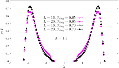
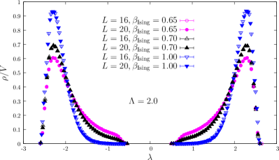
Figure 1: Spectral density of the Ising-Anderson model (reduced) Hamiltonian ${\cal H}^{(+)}$, Eq. (16), for several choices of the parameters $\beta_{\rm Ising}$ and $\Lambda$.

We have performed numerical simulations of the effective Ising-Anderson model discussed in the previous Section, Eqs. (8), (9) and (10). For our purposes it was sufficient to focus on ${\cal H}^{(+)}$, Eq. (16), which contains all the relevant information on the localisation properties of the eigenmodes. To form an overall picture of the properties of the effective model, we have performed full diagonalisation of the Hamiltonian on medium-size lattices ($L=16$ and $L=20$), for inverse temperatures $\beta_{\rm Ising}=0.65,\,0.70$, in the ordered phase of the continuous-spin Ising system, and spin-fermion coupling $\Lambda=1.5,\,2.0$, on 300 spin configurations. We have furthermore fully diagonalised ${\cal H}^{(+)}$ on lattices of the same size for $\beta_{\rm Ising}=1.0$, well above the critical inverse temperature, setting $\Lambda=2.0$.

In Fig. 1 we show the spectral density per unit volume of the system. Low modes have small spectral density, which rapidly increases as one goes up in the spectrum, as expected. Decreasing the temperature, thus making the system more ordered, decreases the spectral density of low modes, as one expects if these modes are localised on fluctuations of the spin variables. Increasing the spin-fermion coupling enlargens the region where the spectral density is small, again as expected, since it should push the effective gap up in the spectrum. The same effect is obtained by increasing $\beta_{\rm Ising}$, i.e., by making the system more ordered. Notice the symmetry under $\lambda\to-\lambda$ of the average spectrum, which has been discussed in the previous Section. There is apparently also a sharp gap in the spectrum, which is however not very sensitive to $\Lambda$, $\beta_{\rm Ising}$, or to the size of the system. This gap is probably a feature of the effective model, due to the drastic simplifications of the spatial hopping terms; in any case, it is irrelevant for our purposes.

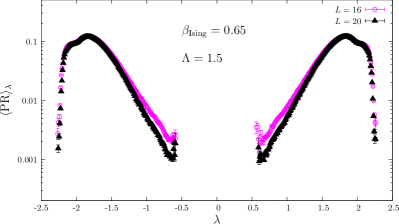
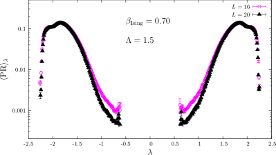
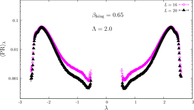
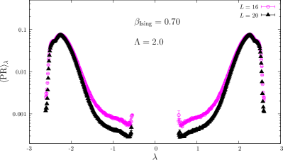
Figure 2: Participation ratio of eigenmodes of the Ising-Anderson model (reduced) Hamiltonian ${\cal H}^{(+)}$, Eq. (16), for $\beta_{\rm Ising}=0.65,\,0.70$ and $\Lambda=1.5,\,2.0$.

In Figs. 2 and 3 we show the average participation ratio ${\rm PR}=\langle(\sum_{x}|\psi(x)|^{4})^{-1}/V\rangle$, which gives a measure of the fraction of space occupied by a given mode, as a function of its location in the spectrum. The ${\rm PR}$ changes by two orders of magnitude as one moves up in the spectrum starting from the low-density region; more importantly, when increasing the size of the system it remains almost constant in the bulk of the spectrum, while it visibly decreases near the origin. This signals that modes in the bulk are delocalised, while modes near the origin are localised. Notice in Fig. 3 the upturn of the ${\rm PR}$ at the low end of the spectrum: a similar phenomenon has been observed in QCD with staggered fermions KP2 .

Finally, in Fig. 4 we show a suitably defined local spectral statistics $I_{\lambda}$ across the spectrum. Spectral statistics can be used to detect a localisation/delocalisation transition, since the eigenvalues corresponding to localised or delocalised eigenmodes are expected to obey different statistics, namely Poisson or Wigner-Dyson statistics, respectively. More precisely, $I_{\lambda}$ is defined as

$$I_{\lambda}=\int_{0}^{\bar{s}}ds\,p_{\lambda}(s)\,,\qquad s_{i}=\frac{\lambda_{i+1}-\lambda_{i}}{\langle\lambda_{i+1}-\lambda_{i}\rangle_{\lambda}}\,,\qquad\bar{s}\simeq 0.473\,,$$ (19)

where the unfolded level spacing distribution (ULSD) $p_{\lambda}(s)$ is the probability distribution, computed locally in the spectrum, of the so-called unfolded level spacing $s_{i}$, i.e., the level spacing divided by the local average level spacing $\langle\lambda_{i+1}-\lambda_{i}\rangle_{\lambda}$. The quantity $I_{\lambda}$ is simply the integrated ULSD up to the crossing point $\bar{s}$ of the exponential distribution, corresponding to Poisson statistics, and the orthogonal Wigner surmise, which accurately describes the ULSD for (orthogonal) Wigner-Dyson statistics. The results confirm that the eigenmodes change from localised to delocalised when one moves up in the spectrum. Moreover, the mobility edge separating localised and delocalised modes goes up in the spectrum when the Ising system is made more ordered by decreasing the temperature, or when the spin-fermion coupling is increased. Our results give also a first indication that the slope of the curve increases as the volume is increased, thus hinting at the existence of a true phase transition in the spectrum. Notice that the transition takes place near the point $\Lambda\frac{1+\langle s_{x}\rangle}{2}$ in the spectrum, thus indicating that the position of the mobility edge is connected to the magnetisation of the system, as expected (see Table 1). This is also in agreement with our expectation for the position of the mobility edge in the “first-order” picture, discussed previously in Section 2.

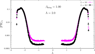
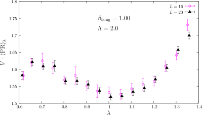
Figure 3: Participation ratio of eigenmodes of the Ising-Anderson model (reduced) Hamiltonian ${\cal H}^{(+)}$, Eq. (16), for $\beta_{\rm Ising}=1.0$ and $\Lambda=2.0$. The right panel is a zoom on the low-lying modes.

To further investigate the onset of critical behaviour, we have determined eigenvalues and eigenvectors on larger volumes ($L=24,\,32,\,40$) in the vicinity of the point in the spectrum where the localisation properties show a dramatic change, for $\beta_{\rm Ising}=1.0$ and $\Lambda=1.5$. We used 20k configurations for $L=24$, scaling down the statistics for larger volumes by keeping approximately constant the total number of eigenvalues computed in the relevant spectral window. In Fig. 5 we show $I_{\lambda}$ as obtained from these simulations: one can easily appreciate the tendency of the cross-over from Poisson to Wigner-Dyson statistics to become steeper as the volume is increased.

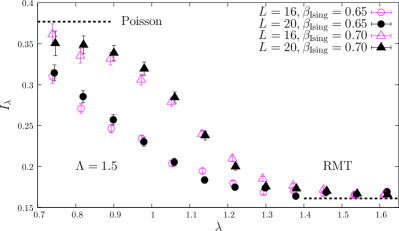
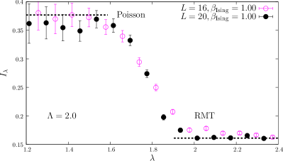
Figure 4: The spectral statistics $I_{\lambda}$, Eq. (19), for the eigenmodes of the Ising-Anderson model (reduced) Hamiltonian ${\cal H}^{(+)}$, Eq. (16), for several choices of $\beta_{\rm Ising}$ and $\Lambda$.

	1.5	2.0
0.65	1.1153(5)	1.4870(7)
0.70	1.1903(3)	1.5871(4)
1.00	1.3386(1)	1.7849(2)

Table 1: Value of $\Lambda\frac{1+\langle s_{x}\rangle}{2}$ corresponding to the various choices of $\beta_{\rm Ising}$ and $\Lambda$ employed in this paper.

Although the data are not of sufficiently good quality to allow a proper finite-size-scaling analysis, it is still possible to make a rough qualitative attempt at showing compatibility of the critical properties with those of the three-dimensional orthogonal Anderson model. According to the one-parameter scaling hypothesis, data from different volumes should collapse on a single curve if plotted against the scaling variable $(\lambda-\lambda_{c})L^{\frac{1}{\nu}}$, where $\lambda_{c}$ is the critical point and $\nu$ the critical exponent of the correlation length. The pretty large distance between the crossing point of the $L=24,\,32$ data and of the $L=32,\,40$ data indicates the presence of sizable finite-size corrections to the position of the critical point, so we limit ourselves to the two largest volumes. In Fig. 5 we show the data collapse for the $L=32,\,40$ data. We determined $\lambda_{c}$ as the crossing point of second-order polynomial fits to the data, and used the value $\nu=1.57$ corresponding to the three-dimensional orthogonal Anderson model nu_orth . Although far from conclusive, this plot shows at least that agreement between the critical properties of the two models is possible.

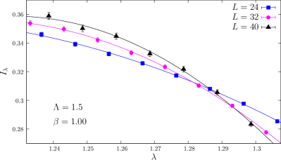
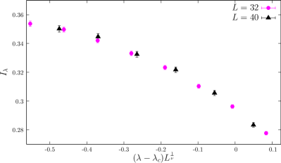
Figure 5: (Left panel) The spectral statistics $I_{\lambda}$, Eq. (19), for the eigenmodes of the Ising-Anderson model (reduced) Hamiltonian ${\cal H}^{(+)}$, Eq. (16), near the critical point in the spectrum. Here $\beta_{\rm Ising}=1.0$ and $\Lambda=1.5$. The solid line is a quadratic fit to the data, and is shown to guide the eye. (Right panel) The same spectral statistics for $L=32,\,40$ plotted against the scaling variable $(\lambda-\lambda_{c})L^{\frac{1}{\nu}}$.

5 Conclusions

In this paper we have discussed a possible mechanism leading to the localisation of low-lying modes of the Dirac operator in the high-temperature phase of QCD. Our proposal is that the localising “traps” are provided by spatial fluctuations (“islands”) of the local Polyakov lines away from the ordered value (i.e., the identity in colour space). In this paper we have generalised the original proposal of Ref. Bruckmann:2011cc to $SU(3)$, which has allowed us to identify the relevant variables for localisation, namely the phases of the eigenvalues of the local Polyakov lines, which govern the “depth” of the localising “traps”. These phases enter the Dirac equation in the form of effective boundary conditions for the quark eigenmodes, and provide a three-dimensional source of disorder. The three-dimensional nature of the “islands”, which constitute disconnected regions in a “sea” of (almost) ordered Polyakov lines, sheds light on the compatibility of the critical properties of the Dirac spectrum at the localisation/delocalisation transition with those of the three-dimensional unitary Anderson model crit .

To further substantiate our proposal, and check the viability of the “sea/islands” explanation, we have reproduced the qualitative features of the localised modes in a three-dimensional effective model, designed to produce localisation precisely through the proposed mechanism. This “Ising-Anderson” model is built replacing the four-dimensional (anisotropic) lattice, appropriate for finite-temperature QCD, with a three-dimensional one, and replacing the temporal covariant derivative in the Dirac operator with a diagonal (on-site) noise. The dynamics of the diagonal noise is governed by an Ising model with continuous spins in the ordered phase, in order to reproduce the qualitative features of the Polyakov line configurations. Localised modes are indeed present, and respond to changes in the parameters (i.e., the temperature of the Ising system and the strength of the spin-fermion coupling) as expected theoretically, thus reinforcing our confidence in the validity of the “sea/islands” explanation in QCD.

There are several possible extensions of the present work. Besides a thorough check of the critical properties of the model at the localisation/delocalisation transition, to be compared with those of the Anderson model in the appropriate symmetry class, the most interesting issue to study is how to properly model the effect of the spatial hopping. As a matter of fact, the diagonal disorder which we believe is responsible for localisation in the high-temperature phase, i.e., the effective boundary conditions, is present also in the low-temperature phase of QCD, but in that case it is ineffective in producing localisation. Indeed, in the low-temperature phase the system looks “fully four-dimensional”, and is basically insensitive to the temporal boundary conditions. In our opinion, in order to understand why this happens, and how the transition between the two phases is realised, adopting the point of view of “QCD as a random-matrix model” held in the present paper, it is necessary to understand how the spatial hopping acts in the two phases, especially concerning its capability of producing delocalised states around the origin. This could lead to useful insights in the subject of chiral symmetry breaking in QCD.

Appendix A Symmetry class of the effective model

The Hamiltonian of our toy model is of the form

$$H=\gamma_{4}A+i\vec{\gamma}\cdot\vec{\partial}\,,$$ (20)

with $A_{\vec{x}\vec{y}}=a_{\vec{x}}\delta_{\vec{x}\vec{y}}$, $a_{\vec{x}}\in\mathbb{R}$, and $(\partial_{j})_{\vec{x}\vec{y}}=\frac{1}{2}(\delta_{\vec{x}+\hat{\jmath},\vec{y}}-\delta_{\vec{x}-\hat{\jmath},\vec{y}})$. In this Appendix Latin indices run from 1 to 3, Greek indices from 1 to 4. We want to find an antiunitary “time-reversal” symmetry of this system. We denote with ${\cal T}$ the corresponding operator, which we parameterise as ${\cal T}=K\Gamma U$, with $K$ the usual complex conjugation and $U$ unitary to be determined, and $\Gamma=\gamma_{5}\gamma_{4}\gamma_{2}$ such that $\Gamma^{\dagger}\gamma_{\mu}^{*}\Gamma=\gamma_{\mu}$, with $\Gamma^{*}=\Gamma$, $\Gamma^{\dagger}\Gamma=\mathbf{1}$ and $\Gamma^{2}=-\mathbf{1}$. We have to impose

$${\cal T}^{\dagger}H{\cal T}=U^{\dagger}\Gamma H^{*}\Gamma U=U^{\dagger}(\gamma_{4}A-i\vec{\gamma}\cdot\vec{\partial})U=\gamma_{4}A+i\vec{\gamma}\cdot\vec{\partial}\,.$$ (21)

Since the last relation has to hold for any choice of $a_{\vec{x}}$, we see that

$$U^{\dagger}\gamma_{4}AU=\gamma_{4}A\,,\qquad U^{\dagger}\vec{\gamma}\cdot\vec{\partial}U=-\vec{\gamma}\cdot\vec{\partial}\,,$$ (22)

by setting $A=0$, and also

$$U^{\dagger}\gamma_{4}U=\gamma_{4}\,,$$ (23)

by setting $a_{\vec{x}}=a$. $U$ must be of the general form

$$U_{\vec{x}\vec{y}}=U^{0}_{\vec{x}\vec{y}}+U^{5}_{\vec{x}\vec{y}}\,\gamma_{5}+\sum_{\mu}U^{\mu}_{\vec{x}\vec{y}}\gamma_{\mu}+\sum_{\mu}\tilde{U}^{\mu}_{\vec{x}\vec{y}}\,i\gamma_{5}\gamma_{\mu}+\sum_{\mu,\nu}V_{\vec{x}\vec{y}}^{\mu\nu}\sigma_{\mu\nu}\,,$$ (24)

where $\sigma_{\mu\nu}=\frac{1}{2i}[\gamma_{\mu},\gamma_{\nu}]$. Imposing Eq. (23) restricts the form of $U$ to

$$U_{\vec{x}\vec{y}}=U^{0}_{\vec{x}\vec{y}}+U^{4}_{\vec{x}\vec{y}}\,\gamma_{4}+\sum_{j}\tilde{U}^{j}_{\vec{x}\vec{y}}\,i\gamma_{5}\gamma_{j}+\sum_{i,j}V^{ij}_{\vec{x}\vec{y}}\,\sigma_{ij}\,.$$ (25)

Plugging this into the first equation in Eq. (22) we obtain

$$(a_{\vec{x}}-a_{\vec{y}})U_{\vec{x}\vec{y}}=0\,,$$ (26)

which implies

$$U_{\vec{x}\vec{y}}={\cal U}_{\vec{x}}\,\delta_{\vec{x}\vec{y}}\,,\qquad{\cal U}_{\vec{x}}=u^{0}_{\vec{x}}+u^{4}_{\vec{x}}\gamma_{4}+\sum_{j}\tilde{u}^{j}_{\vec{x}}\,i\gamma_{5}\gamma_{j}+\sum_{i,j}v^{ij}_{\vec{x}}\sigma_{ij}\,.$$ (27)

Using now the second equation in Eq. (22) we obtain, for the non-vanishing entries with $\vec{y}=\vec{x}\pm\hat{\jmath}$,

$${\cal U}_{\vec{x}\pm\hat{\jmath}}=-\gamma_{j}\,{\cal U}_{\vec{x}}\,\gamma_{j}~{}~{}~{}\text{(no sum over $j$)}\,.$$ (28)

This imposes the following equations,

$$u^{0}_{\vec{x}+\hat{\jmath}} =-u^{0}_{\vec{x}}\,, \tilde{u}^{k}_{\vec{x}+\hat{\jmath}} =-\tilde{u}^{k}_{\vec{x}}~{}~{}\forall k\neq j\,, v^{kl}_{\vec{x}+\hat{\jmath}} =-v^{kl}_{\vec{x}}~{}~{}\forall k,l\neq j\,,$$ (29)

$$u^{4}_{\vec{x}+\hat{\jmath}} =u^{4}_{\vec{x}}\,, \tilde{u}^{j}_{\vec{x}+\hat{\jmath}} =\tilde{u}^{j}_{\vec{x}}\,, v^{jk}_{\vec{x}+\hat{\jmath}} =v^{jk}_{\vec{x}}\,,$$

which are solved by

$$u^{0}_{\vec{x}} =(-1)^{\sum_{k}x_{k}}u^{0}\,, \tilde{u}^{i}_{\vec{x}} =(-1)^{\left(\sum_{k}x_{k}\right)-x_{i}}\tilde{u}^{i}\,,$$ (30)

$$u^{4}_{\vec{x}} =u^{4}\,, v^{ij}_{\vec{x}} =(-1)^{\left(\sum_{k}x_{k}\right)-x_{i}-x_{j}}v^{ij}\,.$$

However, since $U_{\vec{x}\vec{y}}$ must respect the periodic boundary conditions, for lattices of odd linear size the only possibility is ${\cal U}_{\vec{x}}=e^{i\phi}\gamma_{4}$. Computing the square of the time-reversal operator,

$${\cal T}^{2}=K\Gamma UK\Gamma U=-\Gamma^{\dagger}U^{*}\Gamma U=-(\gamma_{4})^{2}=-\mathbf{1}\,,$$ (31)

so for odd lattices the symmetry class is the symplectic one. For even lattices, it is possible to choose ${\cal U}_{\vec{x}}=e^{i\phi}(-1)^{\sum_{k}x_{k}-x_{j}}i\gamma_{5}\gamma_{j}$ for any $j$, which yields

$${\cal T}^{2}=-(\gamma_{5}\gamma_{j})^{2}=\mathbf{1}\,,$$ (32)

so that the symmetry class is the orthogonal one (the existence of at least one antiunitary symmetry operator with square one is sufficient to see this). Even more simply, after spin diagonalisation the Hamiltonian reads

$${\cal H}_{\vec{x}\vec{y}}=\eta_{4}(\vec{x})A_{\vec{x}\vec{y}}+i\vec{\eta}(\vec{x})\cdot\vec{\partial}_{\vec{x}\vec{y}}\,,$$ (33)

and one can easily identify the time-reversal operator ${\cal T}_{\vec{x}\vec{y}}=\eta_{4}(\vec{x})\delta_{\vec{x}\vec{y}}K$, which has ${\cal T}^{2}=\mathbf{1}$.

References

- (1) T. Banks and A. Casher, Nucl. Phys. B 169 (1980) 103.
- (2) J. J. M. Verbaarschot and T. Wettig, Ann. Rev. Nucl. Part. Sci. 50 (2000) 343 [hep-ph/0003017].
- (3) P. de Forcrand, AIP Conf. Proc. 892 (2007) 29 [hep-lat/0611034].
- (4) T. G. Kovács and F. Pittler, Phys. Rev. D 86 (2012) 114515 [arXiv:1208.3475 [hep-lat]].
- (5) M. Giordano, T. G. Kovács and F. Pittler, PoS LATTICE 2013 (2013) 212 [arXiv:1311.1770 [hep-lat]].
- (6) A. M. García-García and J. C. Osborn, Nucl. Phys. A 770 (2006) 141 [hep-lat/0512025].
- (7) A. M. García-García and J. C. Osborn, Phys. Rev. D 75 (2007) 034503 [hep-lat/0611019].
- (8) T. G. Kovács, Phys. Rev. Lett. 104 (2010) 031601 [arXiv:0906.5373 [hep-lat]].
- (9) T. G. Kovács and F. Pittler, Phys. Rev. Lett. 105 (2010) 192001 [arXiv:1006.1205 [hep-lat]].
- (10) Y. Aoki, Z. Fodor, S. D. Katz and K. K. Szabó, Jour. High Energy Phys. 01 (2006) 089 [hep-lat/0510084].
- (11) S. Borsányi, G. Endrődi, Z. Fodor, A. Jakovác, S. D. Katz, S. Krieg, C. Ratti and K. K. Szabó, Jour. High Energy Phys. 11 (2010) 077 [arXiv:1007.2580 [hep-lat]].
- (12) G. Cossu et al. [JLQCD Collaboration], arXiv:1412.5703 [hep-lat].
- (13) M. Giordano, T. G. Kovács, S. D. Katz and F. Pittler, arXiv:1410.8392 [hep-lat].
- (14) P. de Forcrand and O. Philipsen, Jour. High Energy Phys. 11 (2008) 012 [arXiv:0808.1096 [hep-lat]].
- (15) M. Giordano, T. G. Kovács and F. Pittler, Phys. Rev. Lett. 112 (2014) 102002 [arXiv:1312.1179 [hep-lat]].
- (16) P. W. Anderson, Phys. Rev. 109 (1958) 1492.
- (17) P. A. Lee and T. V. Ramakrishnan, Rev. Mod. Phys. 57 (1985) 287.
- (18) F. Evers and A. D. Mirlin, Rev. Mod. Phys. 80 (2008) 1355 [arXiv:0707.4378 [cond-mat.mes-hall]].
- (19) M. Mehta, Random Matrices (Academic Press, San Diego, 1991).
- (20) K. Slevin and T. Ohtsuki, Phys. Rev. Lett. 78 (1997) 4083 [cond-mat/9704192 [cond-mat.dis-nn]].
- (21) E. N. Economou, P. D. Antoniou, Solid State Commun. 21 (1977) 285.
- (22) D. Weaire and V. Srivastava, Solid State Commun. 23 (1977) 863.
- (23) F. Bruckmann, T. G. Kovács and S. Schierenberg, Phys. Rev. D 84 (2011) 034505 [arXiv:1105.5336 [hep-lat]].
- (24) A. Roberge and N. Weiss, Nucl. Phys. B 275 (1986) 734.
- (25) P. de Forcrand and O. Philipsen, Nucl. Phys. B 642 (2002) 290 [hep-lat/0205016].
- (26) M. D’Elia and M. P. Lombardo, Phys. Rev. D 67 (2003) 014505 [hep-lat/0209146].
- (27) A. M. García-García and E. Cuevas, Phys. Rev. B 74 (2006) 113101 [cond-mat/0602331 [cond-mat.dis-nn]].
- (28) L. G. Yaffe and B. Svetitsky, Phys. Rev. D 26 (1982) 963.
- (29) T. A. DeGrand and C. E. DeTar, Nucl. Phys. B 225 (1983) 590.
- (30) K. Slevin and T. Ohtsuki, Phys. Rev. Lett. 82 (1999) 382 [cond-mat/9812065 [cond-mat.dis-nn]].