Analysing the effects of apodizing windows on local correlation tracking using Nirvana simulations of convection

Abstract

We employ different shapes of apodizing windows in the local correlation tracking (LCT) routine to retrieve horizontal velocities using numerical simulations of convection. LCT was applied on a time sequence of temperature maps generated by the Nirvana code with four different apodizing windows, namely–Gaussian, Lorentzian, trapezoidal and triangular, with varying widths. In terms of correlations (between the LCT-retrieved and simulated flow field), the triangular and the trapezoidal perform the best and worst, respectively. On segregating the intrinsic velocities in the simulations on the basis of their magnitudes, we find that for all windows, a significantly higher correlation is obtained for the intermediate and high-velocity bins and only modest or weak values in the low-velocity bins. The differences between the LCT-retrieved and simulated flow fields were determined spatially which show large residuals at or close to the boundary of granules. The extent to which the horizontal flow vectors retrieved by LCT compare with the simulated values, depends entirely on the width of the central peak of the apodizing window for a given $\sigma$. Even though LCT suffers from a lack of spatial content as seen in simulations, its simplicity and speed could serve as a viable first-order tool to probe horizontal flows–one that is ideal for large data sets.

1 Introduction

intro High-resolution observations of solar granulation from the balloon-borne solar observatory SUNRISE (Barthol et al., 2011) reveal sub-structures such as granular lanes which typically consist of a bright and a dark edge, that travel from the visible boundary of granules into the granule itself (Steiner et al., 2010). By comparing the observations with numerical simulations, Steiner et al. (2010) interpret these structures to be signatures of vortex tubes which are a fundamental structure element of turbulence and are important for transferring energy from large to small scales. On the other hand, granules are also considered good tracers of the large-scale flows (Stangalini, 2014), particularly that of supergranular flows (Hart, 1956). Leighton, Noyes, and Simon (1962) and Simon and Leighton (1964) showed that the edges of supergranular cells coincide with the chromospheric emission network. This suggests that the large-scale horizontal flow is responsible for advecting magnetic fields along the network boundaries. Solar granulation thus serves as a proxy for the transport of small-scale magnetic fields and their subsequent accumulation and intensification at the network. Hence it is important to have tools that can identify and track granular flows on the solar surface.

There are several methods to track solar granulation. Of these, local correlation tracking (LCT; November, 1986; November and Simon, 1988; Welsch et al., 2004; Fisher and Welsch, 2008) is the oldest and most commonly used routine. LCT computes the relative displacement of small sub-regions centred on a particular pixel. A Gaussian window, whose full-width-at-half-maximum (FWHM) needs to be roughly the size of the structures that are to be tracked, is used to apodize the sub-regions. Thus, the horizontal speed at each pixel can be determined knowing the displacement, image scale, and the time interval. The “balltracking” method of Potts, Barrett, and Diver (2004) also produces results with the same accuracy as LCT but is significantly more efficient, computationally. On the other hand, the feature-tracking routine of Strous (1995) allows the determination of physical characteristics of individual small features. Other tracking routines include the induction method (IM; Kusano et al., 2002), inductive local correlation tracking (ILCT; Welsch et al., 2004), Fourier local correlation tracking (FLCT; Welsch et al., 2004), minimum-energy fit (MEF; Longcope, 2004), minimum-structure reconstruction (MSR; Georgoulis and LaBonte, 2006) method, differential affine velocity estimator (DAVE; Schuck, 2006), and nonlinear affine velocity estimator (NAVE; Schuck, 2005). All these techniques, except FLCT, are based on the ideal induction equation and are used to track the magnetic footpoint velocity using magnetograms. Welsch et al. (2007) performed tests with the above routines (except NAVE) on synthetic magnetograms generated from anelastic MHD simulations of Lantz and Fan (1999) and concluded that DAVE estimated the magnitude and direction of velocities slightly more accurately than the other methods, while MEF’s estimates of the fluxes of magnetic energy and helicity were far more accurate than the others. While the above methods have varying computational demands, LCT is the fastest routine among these.

Verma, Steffen, and Denker (2013) used simulated continuum images from the CO⁵BOLD code (Freytag et al., 2012) to compare plasma flows with those retrieved by LCT. A similar analysis was performed by Yelles Chaouche, Moreno-Insertis, and Bonet (2014) using synthetic continuum maps generated by the STAGGER code (Beeck et al., 2012). The above studies reveal that the horizontal proper motions are not effectively retrieved by LCT. This drawback has been attributed to the nature of granules whose motions are representative of the large-scale plasma flow for length and time scales greater than 2.5 Mm and 30 min, respectively (Rieutord et al., 2001). While the comparison of horizontal flows retrieved from LCT on synthetic data is the best way to validate the method and to determine its limitations, it is not overtly clear if the proper motions derived from LCT can and should be compared directly with simulated horizontal plasma motions. Firstly, LCT tracks contrast fluctuations between two images which is not the same as the underlying plasma motions. Secondly, LCT only determines the relative displacement between two images, that are separated in time and for a pixel of interest. The resultant morphology would thus reflect displacements and not velocity, despite using a constant scaling factor (arising from the spatial sampling and time step) for all pixels in the field of view. Thirdly, LCT is formally not consistent with the normal component of the induction equation, which can be expressed as a continuity equation; but rather with the advection equation (Schuck, 2005). Furthermore, it is not known if a Gaussian apodizing window is or would be the best choice when using LCT.

In this paper, we evaluate the performance of LCT on convection simulations for different shapes of apodizing windows, taking advantage of the fact that LCT is the simplest and one of the most computationally efficient velocity determination tools. Our aim is to determine whether a different apodizing function can significantly improve LCT results which could then be used in future studies. Such a study, to the best of our knowledge, has not been carried out previously. As a secondary product of these tests, we also validate LCT and discuss its advantages and limitations with respect to simulations, as well as its implications for solar observations.

2 Nirvana simulations of convection

nirv The two-dimensional (2D) images showing temperature and horizontal velocity components in Figure fig01 are snapshots from a three-dimensional box simulation of magneto-convection in a stratified gas layer. The simulation box is rectangular and contains two layers of gas. The temperature stratification is convectively unstable in the upper layer and stable in the lower layer. The Rayleigh number in the unstable layer is $10^{7}$, the thermal and magnetic Prandtl numbers both assume values of 0.1. Density and temperature both assume values of the order one while the isothermal sound speed is 100 and the pressure increases from 10⁴ at the top to 10⁵ at the bottom. The magnetic field is vertical and the field strength has been chosen to be near equipartition with the gas density at the top of the box.

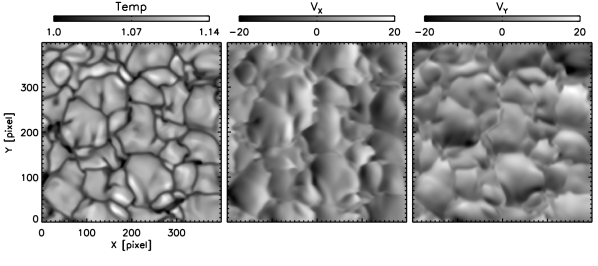
Figure 1.: Left panel: Snapshot of temperature from the Nirvana simulation. The corresponding x- and y-components of the velocity vector are shown in the middle and right panels, respectively.fig01

The setup is the same as used in Rüdiger, Küker, and Schnerr (2012). We use the Nirvana MHD code (Ziegler, 2004) to solve the equation of motion, the induction equation, and the conservation equations for mass and energy in Cartesian coordinates for an ideal gas of constant molecular weight. The aspect ratio of the simulation box is $8\times 8\times 2$ in the $x$, $y$, and $z$ coordinates. Stratification is along the $z$ axis with the gravity vector pointing in the negative direction, i.e. the $z$ axis pointing upwards. The bottom of the box is at $z=-2$, the top at $z=0$. The horizontal cross sections were taken at $z=-0.05$.

The boundary conditions are periodic in the horizontal ($x$ and $y$) directions. The vertical ($z$) boundary conditions prevent outflow, i.e. specify zero mass flow across the boundaries, and stress-free in the horizontal components. The temperature is kept fixed at the upper boundary while the heat flux is prescribed at the lower boundary. We use a mesh with $513\times 513\times 128$ points. The computations have been carried out in the AIP’s Leibniz cluster using the message passing interface with 256 CPU cores in parallel. Dimensionless units have been used for all quantities.

The time separation in the simulations was chosen to be sufficiently smaller than the characteristic time scale of the granules and to have a high correlation between successive frames, so as perform tracking on consecutive temperature maps. The temperature distribution exhibits two clear peaks which correspond to the dark cell boundaries and the granules which represent upflowing plasma. Since temperature is a dimensionless quantity, converting it into bolometric intensity, to derive the image contrast, is not possible. A proxy for the contrast was however done in the following manner. The two-peak distribution was fitted with two Gaussians, whose mean and $\sigma$ are represented as $m_{1}$, $\sigma_{1}$ and $m_{2}$, $\sigma_{2}$, respectively. If $<I>$ represents the mean value of the image then the contrast is expressed as $((m_{2}+\sigma_{2})-(m_{1}-\sigma_{1}))/<I>$. Using this expression, the contrast is estimated to be about 6%. In comparison the contrast for solar granulation is about 14% at 630 nm as shown by Danilovic et al. (2008) using MHD simulations.

Figure 2.: Different shapes of apodizing windows used in LCT. The 1D profiles correspond to a $\sigma=10$ pixel.fig02b

3 Apodizing windows for LCT

apod Inferring the velocity of features from a set of two images depends on two parameters, namely, the apodizing window function and the time difference between the two images. Before computing the cross correlation, the first step is to generate the apodizing window function with a given width ($\sigma$). The window function is multiplied with sub-images in the reference frame and the object frame, thus smoothing both the sub-images. The apodization also restricts the motion of the features to the window size. The choice of the time step depends on the evolution time scale of the feature, as a small time step might yield a poor correlation owing to a small shift, while a large time step could render the feature outside the apodizing window. Thus, a compromise between the width of the apodizing window and the time difference is necessary.

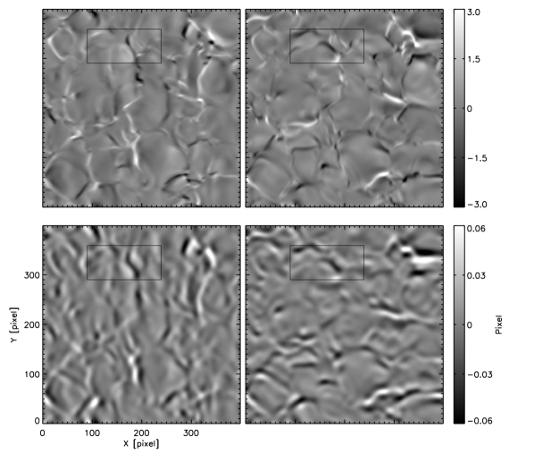
Figure 3.: Top panels: Velocity-difference maps in x-(left) and y-directions (right) obtained from successive frames of the simulation sequence. Bottom panels: Example of horizontal velocities obtained after LCT was applied to the corresponding temperature maps. A Gaussian window of $\sigma=10$ pixel was used in this case. The black rectangle in the panels corresponds to a smaller region shown in Figure fig04.fig02

In order to compute the shifts, we used a Fast Fourier Transform (FFT) based cross-correlation program (Nisenson et al., 2003). The displacements were determined with sub-pixel accuracy by fitting a quadratic function to the cross-correlated values near the peak. This procedure yields displacement vectors for all pixels in each frame and for the entire time sequence. The program is very fast and on a 3.2 GHz Intel-core processor, it takes about 70 sec for a Gaussian apodizing window having a width of $\sigma=15$ pixel and for an image of size 513$\times$513 pixel. We generated 2D Gaussian, Lorentzian, trapezoidal and triangular windows for widths of $\sigma=$ 10, 15, and 20 pixel. The windows were constructed such that for a given $\sigma$, the FWHM was the same for all, thus providing a basis for comparison. This is shown in Figure fig02b for a one-dimensional (1D) plot of each window function for a width of $\sigma=10$ pixel.

Figure 4.: Linear correlations between simulated velocities and that derived by LCT. Top panels: Correlation coefficients in the $x$-direction as a function of time for different apodizing windows, shown with different symbols and inscribed in the left-most panel. Panels from left to right correspond to different widths of the apodizing window. Bottom panels: Same as above but for the $y$-direction.fig03

As mentioned in Section nirv the tracking was done on successive frames as we were interested in retrieving the instantaneous horizontal motions. The central 400$\times$400 pixel region was chosen for analysis to avoid the edges that were affected by the apodization. The top panels of Figure fig02 show running-difference maps of the simulated horizontal velocity from successive frames, while the bottom panel shows the displacements determined by LCT using a Gaussian apodizing window with a width of $\sigma=10$ pixel. The running-difference velocity maps, thus, reflect displacements, albeit with time as a dimensionless scale factor, and henceforth we will refer to them as velocities, unless otherwise stated.

4 Results

res

4.1 Correlations between LCT-retrieved and simulated horizontal velocities

compare We compute the Pearson linear correlation coefficient (CC) of the horizontal velocities retrieved by LCT and simulations for the different apodizing windows and widths for the entire time sequence. Figure fig03 shows that the correlations in both $x$- and $y$-directions have a time-dependent behaviour which is reflected very similarly in all apodizing windows and for all widths considered. This time-dependence of the CCs is related to the temporal evolution of the convective pattern seen in the simulated velocity-difference maps. The correlation decreases as the width of the apodizing window increases. For the narrowest window having a width of $\sigma=10$ pixel, the correlation is the highest and nearly the same for all the apodizing windows. However, as the width of the window increases, we find a distinction in the correlations, the highest being for the Lorentzian and triangular apodizing windows, followed closely by the Gaussian and being the lowest for the trapezoidal window.

The maximum CCs for the Gaussian, Lorentzian, and triangular windows are about 0.64 in both the $x$- and $y$-directions for a width of $\sigma=10$ pixel, while the corresponding minimum values are 0.52 and 0.50, respectively. Similar values are seen with the trapezoidal window for the same width. With the exception of the trapezoidal window, where the minimum value of the CC is quite low for the largest width, the same is relatively modest for the triangular, Lorentzian and Gaussian windows. The difference between the maximum (or minimum) CCs for $\sigma=10$ and 20 pixel vary by about 20% for the trapezoidal apodizing window, while this variation is only about 10% for the other three windows. Although, we find a time dependence in the CCs, the minimum and maximum values of the CC for the triangular, Lorentzian and Gaussian apodizing windows differ by about 15%.

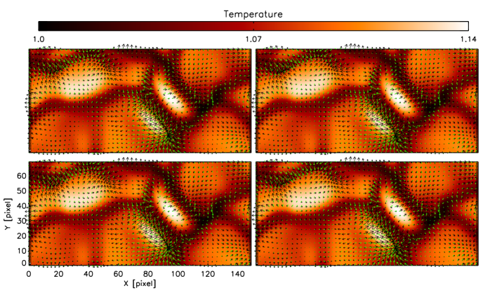
Figure 5.: Comparison of horizontal flow vectors from LCT (black arrows) and simulations (green arrows) for the area indicated by the black box in Figure fig02. The arrows have been drawn for every third pixel and overlaid on the corresponding temperature map. Top panels – Gaussian (left) and Lorentzian (right) apodizing windows. Bottom panels - trapezoidal (left) and trianglular (right) apodizing windows.fig04

4.2 Comparison of flow vectors

scale As mentioned in Section nirv, the physical parameters are dimensionless and in order to make a pixel-to-pixel comparison of the simulated velocities with those from LCT, we determined the scale factor relating the two quantities, from a linear regression fit to the scatter plot (not shown) in the $x$- and $y$-directions. The above exercise was performed for each map in the time sequence. Using the regression gradient as a scale factor, the horizontal flow field from the simulations and that from LCT can be directly compared and is illustrated in Figure fig04 for all windows with a width of $\sigma=10$ pixel. We find that the flow vectors from LCT are in concordance with those from simulations. As seen earlier in Figure fig02, the horizontal velocities retrieved from LCT lack the fine structure as observed in the simulated data although there is an overall morphological agreement between the two and this is the reason for the modest correlation shown in Figure fig03. Subsequently, the LCT flow vectors appear stronger than the simulated ones particularly at locations where the intrinsic velocities are high. The movie also shows the temporal evolution of the simulated flows, which match the LCT-determined flows quite well. It is observed that the flow maps retrieved by LCT using the trapezoidal window are weaker in amplitude and spatially smoother in comparison to the other three windows.

Table 1.: Correlation coefficients for different windows and widths for different simulated velocity bins in the $x$- and $y$-directions for the entire time sequence. Gau–Gaussian, Lor–Lorentzian, Tap–trapezoidal, Tri–triangle.

Velocity range	$\sigma=10$				$\sigma=15$				$\sigma=20$
	Gau	Lor	Tap	Tri	Gau	Lor	Tap	Tri	Gau	Lor	Tap	Tri
$|V_{x}|<0.5$	0.43	0.42	0.43	0.43	0.47	0.47	0.44	0.48	0.46	0.47	0.39	0.48
$0.5\leq|V_{x}|\leq 1.5$	0.70	0.70	0.70	0.70	0.68	0.69	0.62	0.69	0.60	0.63	0.46	0.64
$|V_{x}|>1.5$	0.79	0.79	0.78	0.79	0.74	0.76	0.67	0.76	0.62	0.67	0.36	0.69
$|V_{y}|<0.5$	0.43	0.41	0.43	0.43	0.47	0.47	0.44	0.48	0.46	0.47	0.39	0.48
$0.5\leq|V_{y}|\leq 1.5$	0.70	0.69	0.70	0.70	0.68	0.69	0.62	0.69	0.60	0.63	0.47	0.64
$|V_{y}|>1.5$	0.79	0.79	0.78	0.79	0.74	0.75	0.65	0.76	0.60	0.66	0.35	0.68

tab2

4.3 Velocity-dependent LCT values

velo Following Figure fig04, we investigate if the correlations between simulated and LCT velocities depend on the intrinsic magnitude of the flows since the values determined in Section compare considers the entire distribution of velocities. This test serves to check if LCT can recover smaller velocities with the same accuracy as larger ones. From the histogram of the simulated velocities, we selected three bins corresponding to $|V|<0.5$, $0.5\leq|V|\leq 1.5$ and $|V|>1.5$ which represent low, intermediate and high velocities, respectively in both $x$- and $y$-directions. The three bins represent about 78.8%, 19.2% and 2.0% of the 2D velocity distribution, respectively in both directions and in time. Here, 2% corresponds to a sample of 3200 pixels. Note that the velocity bins described above correspond to dimensionless values and were chosen by hand from the velocity distribution. Table tab2 summarizes the CCs between the simulated velocities and those from LCT for the three velocity bins and it is evident that when considered separately, the correlations improve significantly, becoming strong especially for the intermediate and high velocity bins. Thus, the modest correlations obtained in Section compare are due to the low/weak velocities which dominate the distribution. The CCs for all windows and for the smallest width of $\sigma=10$ pixel are about 0.70 and 0.79 for the intermediate and high velocity bins, respectively in both $x$- and $y$-directions. Even in the case of the largest width($\sigma=20$ pixel), the CC, with the exception of the trapezoidal window, is greater than 0.6 for both $x$- and $y$-directions. The CCs are nearly independent of the width for all windows, in the low velocity bin and in both directions, the variation being less than 5%. Even though the spatial domain is dominantly populated by weaker velocities, the global regression coefficient, described in Section scale, is representative of the same from the intermediate velocity bin.

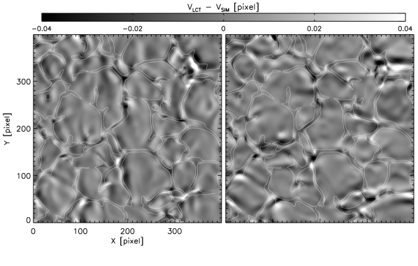
Figure 6.: Left panel: Spatial difference maps between LCT and simulated velocities in the $x$-direction for the triangular apodizing window. Right panel: Same as left panel but for the $y$-direction. The scaling of the images is indicated in the color bar. The maps correspond to a width of $\sigma=10$ pixel. The contours correspond to a temperature of 1.05 and outline most of the intergranular lanes.fig05

4.4 Spatial distribution of velocity differences

spatial Figure fig05 shows a difference map of the horizontal velocities from simulations and those derived from LCT, in $x$- and $y$-directions, using the triangular apodizing window, for $\sigma=10$ pixel. This is also representative of the maps obtained with the Lorentzian and Gaussian windows of the same width. The relevant scale factor described in Section scale was used for the simulated velocity map and in the figure, black(white) represents strong negative(positive) residuals. Using the contours from the corresponding temperature map, we find that the locations of good agreement are confined to granules which represent upflowing material, while regions with strong residuals are located at or close to the boundaries of the granular cells. These residuals occur at specific locations in the field of view and not at all cell boundaries. On a closer inspection of the flow vectors obtained from LCT and those from simulations reveal that there are subtle differences between the two even at the location of granules but the inherent, weak horizontal flows mask the small residuals in comparison to that seen at the inter-granular lanes.

5 Discussion

discuss We have used numerical simulations of convection to analyse the performance of LCT for different shapes of apodizing windows as such a study has not been carried out previously. Since the horizontal velocities are known from simulations, they can be compared with those retrieved by LCT and the latter was applied to the simulated temperature maps so as to mimic the situation often used in solar observations. We first discuss the effects introduced by the different apodizing windows and follow it up with the validation of LCT on the simulated data.

5.1 Performance of different apodizing windows

wind LCT was used on the simulations with four different shapes of apodizing windows, namely–Gaussian, Lorentzian, trapezoidal, and triangular, with different widths. The width of the apodizing window is related to the size of the structure to be tracked and hence will vary on the spatial resolution. As the temperature maps from the simulations have significant structural detail and are not affected by instrumental and atmospheric effects, it is clear that the narrowest windows (albeit still significantly larger than the size element) would give better results. This was indeed the case, as all four windows perform nearly the same for the narrowest width, which is in agreement with Verma, Steffen, and Denker (2013), who used a Gaussian apodizing window function. Indeed, we have performed the above tests for a width of $\sigma=5$ pixel and found that although the results from all the windows yield the same correlation coefficient, the values are less than that observed in the $\sigma=10$ or 15 pixel case. The lower correlations obtained with a width of $\sigma=5$ pixel, imply that the displacement of the features exceeds the width of the window. We also examined the case when $\sigma$ was increased to 25 pixel and found that the correlations decrease further than the $\sigma=20$ pixel case with a similar separation of values amongst the four windows. The above suggest that apodizing widths within the range of 10 and 15 pixels are optimal for tracking intensity features in the simulations.

The Gaussian window was only marginally inferior to the triangular and Lorentzian windows in terms of the correlations obtained. However the correlations from these three window functions were less sensitive to the width than the trapezoidal window. This could be attributed entirely to the width of the peak centred on the pixel of interest, for a given $\sigma$. The outer wings or edges of the window do not affect the results as long as the window is wide enough to detect the motion of the structure in the chosen time step. The triangular window has an abrupt cut-off at its edge, while its peak has the smallest width, and retrieves the same, albeit marginally better, result than the Lorentzian and Gaussian windows, both of which have comparatively extended wings. By the same argument, the central peak or plateau of the trapezoidal window increases more rapidly with $\sigma$, which would explain why the correlations obtained with it are lower than the others.

5.2 Validation of LCT

valid The uniform image quality and high spatial content in the simulations allowed us to track consecutive frames thus eliminating the need to vary the time step. In fact, the effectiveness of the tracking routine is established by the accuracy of the instantaneous flow field retrieved from successive frames and has critical physical implications for understanding energy transfer in the Sun at small, spatial, and temporal scales (Steiner et al., 2010; Moll, Cameron, and Schüssler, 2011). As the simulations presented here are dimensionless, it limits a direct comparison in terms of physical units that can be checked with those known from solar observations. This limitation aside, the comparison of results from LCT and simulations can be regarded as impartial and unbiased.

We reiterate that LCT only retrieves relative displacements between two sub-images and as such should strictly be compared with a running-difference of velocity and not directly with velocity itself. Applying a scale factor to obtain velocity from the LCT results will not in any way alter the nature of the horizontal flows. This would explain why the results obtained by Verma, Steffen, and Denker (2013) vary significantly. Even though the LCT flow maps appear to be a smoother version of that seen in simulations, there is an overall morphological agreement, which could be the reason for the moderate-to-high correlations obtained in our analysis. Despite this drawback, the fact that LCT is relatively simple and not computationally intensive, makes it a viable diagnostic tool for probing horizontal flows. The lack of fine structure in the LCT horizontal flow maps can explain the results of Yelles Chaouche, Moreno-Insertis, and Bonet (2014) who found that the Fourier spectra for the LCT-determined velocities is well below that from the actual velocity components. We have not carried out any spatial smoothing of the simulated data as Verma, Steffen, and Denker (2013) but have performed a pixel-to-pixel comparison. Our analysis also reveals that when the intrinsic velocities are sufficiently strong, the accuracy of LCT is also higher as reflected in the correlations corresponding to different velocity bins.

The spatial differences in the LCT-determined flow fields and simulations reveal that large residuals can occur close to or at the edge of the granular boundaries with very small differences at the granules themselves as also seen in Welsch et al. (2007). This suggests that such sites could possibly reflect interesting physical processes that could be the topic of further investigation by employing other computationally intensive tracking routines.

6 Conclusions

conclu We have tested the conventional use of a Gaussian apodizing window in LCT against other shapes of windows and found that for a given $\sigma$, the width of the peak centred on the pixel of interest influences the determination of the horizontal motions. On the basis of this result, the triangular window yields the best result while the trapezoidal, the worst. The LCT routine was tested on simulations of convection but it remains to be seen if a similar result can be obtained with magneto-convective simulations which replicate solar-like conditions (Vögler et al., 2005; Rempel et al., 2009; Cheung et al., 2010). In the course of this analysis we also tested the validity of LCT in determining known plasma motions and we conclude that LCT can still be used as a first-order approach to derive horizontal proper motions that is ideal for processing large data sets.

Acknowledgements

R. E. L is grateful for the financial assistance from the German Science Foundation (DFG) under grant DE 787/3-1 and the European Commission’s FP7 Capacities Programme under Grant Agreement number 312495. M. K. G acknowledges support by the European Commission’s FP7 Marie Curie Programme under grant agreement no. PIRG07-GA-2010-268245. This work used the Nirvana code developed by Dr. Udo Ziegler at the Leibniz-Institut für Astrophysik Potsdam (AIP). We thank the referee for the useful suggestions and comments.

References

- Barthol et al. (2011) Barthol, P., Gandorfer, A., Solanki, S.K., Schüssler, M., Chares, B., Curdt, W., Deutsch, W., Feller, A., Germerott, D., Grauf, B., Heerlein, K., Hirzberger, J., Kolleck, M., Meller, R., Müller, R., Riethmüller, T.L., Tomasch, G., Knölker, M., Lites, B.W., Card, G., Elmore, D., Fox, J., Lecinski, A., Nelson, P., Summers, R., Watt, A., Martínez Pillet, V., Bonet, J.A., Schmidt, W., Berkefeld, T., Title, A.M., Domingo, V., Gasent Blesa, J.L., Del Toro Iniesta, J.C., López Jiménez, A., Álvarez-Herrero, A., Sabau-Graziati, L., Widani, C., Haberler, P., Härtel, K., Kampf, D., Levin, T., Pérez Grande, I., Sanz-Andrés, A., Schmidt, E.: 2011, The Sunrise Mission. Sol. Phys. 268, 1. DOI. ADS.
- Beeck et al. (2012) Beeck, B., Collet, R., Steffen, M., Asplund, M., Cameron, R.H., Freytag, B., Hayek, W., Ludwig, H.-G., Schüssler, M.: 2012, Simulations of the solar near-surface layers with the CO5BOLD, MURaM, and Stagger codes. A&A 539, A121. DOI. ADS.
- Cheung et al. (2010) Cheung, M.C.M., Rempel, M., Title, A.M., Schüssler, M.: 2010, Simulation of the Formation of a Solar Active Region. ApJ 720, 233. DOI. ADS.
- Danilovic et al. (2008) Danilovic, S., Gandorfer, A., Lagg, A., Schüssler, M., Solanki, S.K., Vögler, A., Katsukawa, Y., Tsuneta, S.: 2008, The intensity contrast of solar granulation: comparing Hinode SP results with MHD simulations. A&A 484, L17. DOI. ADS.
- Fisher and Welsch (2008) Fisher, G.H., Welsch, B.T.: 2008, FLCT: A Fast, Efficient Method for Performing Local Correlation Tracking. In: Howe, R., Komm, R.W., Balasubramaniam, K.S., Petrie, G.J.D. (eds.) Subsurface and Atmospheric Influences on Solar Activity, Astronomical Society of the Pacific Conference Series 383, 373. ADS.
- Freytag et al. (2012) Freytag, B., Steffen, M., Ludwig, H.-G., Wedemeyer-Böhm, S., Schaffenberger, W., Steiner, O.: 2012, Simulations of stellar convection with CO5BOLD. Journal of Computational Physics 231, 919. DOI. ADS.
- Georgoulis and LaBonte (2006) Georgoulis, M.K., LaBonte, B.J.: 2006, Reconstruction of an Inductive Velocity Field Vector from Doppler Motions and a Pair of Solar Vector Magnetograms. ApJ 636, 475. DOI. ADS.
- Hart (1956) Hart, A.B.: 1956, Motions in the Sun at the photospheric level. VI. Large-scale motions in the equatorial region. MNRAS 116, 38. ADS.
- Kusano et al. (2002) Kusano, K., Maeshiro, T., Yokoyama, T., Sakurai, T.: 2002, Measurement of Magnetic Helicity Injection and Free Energy Loading into the Solar Corona. ApJ 577, 501. DOI. ADS.
- Lantz and Fan (1999) Lantz, S.R., Fan, Y.: 1999, Anelastic Magnetohydrodynamic Equations for Modeling Solar and Stellar Convection Zones. ApJS 121, 247. DOI. ADS.
- Leighton, Noyes, and Simon (1962) Leighton, R.B., Noyes, R.W., Simon, G.W.: 1962, Velocity Fields in the Solar Atmosphere. I. Preliminary Report. ApJ 135, 474. DOI. ADS.
- Longcope (2004) Longcope, D.W.: 2004, Inferring a Photospheric Velocity Field from a Sequence of Vector Magnetograms: The Minimum Energy Fit. ApJ 612, 1181. DOI. ADS.
- Moll, Cameron, and Schüssler (2011) Moll, R., Cameron, R.H., Schüssler, M.: 2011, Vortices in simulations of solar surface convection. A&A 533, A126. DOI. ADS.
- Nisenson et al. (2003) Nisenson, P., van Ballegooijen, A.A., de Wijn, A.G., Sütterlin, P.: 2003, Motions of Isolated G-Band Bright Points in the Solar Photosphere. ApJ 587, 458. DOI. ADS.
- November (1986) November, L.J.: 1986, Measurement of geometric distortion in a turbulent atmosphere. Appl. Opt. 25, 392. DOI. ADS.
- November and Simon (1988) November, L.J., Simon, G.W.: 1988, Precise proper-motion measurement of solar granulation. ApJ 333, 427. DOI. ADS.
- Potts, Barrett, and Diver (2004) Potts, H.E., Barrett, R.K., Diver, D.A.: 2004, Balltracking: An highly efficient method for tracking flow fields. A&A 424, 253. DOI. ADS.
- Rempel et al. (2009) Rempel, M., Schüssler, M., Cameron, R.H., Knölker, M.: 2009, Penumbral Structure and Outflows in Simulated Sunspots. Science 325. DOI. ADS.
- Rieutord et al. (2001) Rieutord, M., Roudier, T., Ludwig, H.-G., Nordlund, Å., Stein, R.: 2001, Are granules good tracers of solar surface velocity fields? A&A 377, L14. DOI. ADS.
- Rüdiger, Küker, and Schnerr (2012) Rüdiger, G., Küker, M., Schnerr, R.S.: 2012, Cross helicity at the solar surface by simulations and observations. A&A 546, A23. DOI. ADS.
- Schuck (2005) Schuck, P.W.: 2005, Local Correlation Tracking and the Magnetic Induction Equation. ApJ 632, L53. DOI. ADS.
- Schuck (2006) Schuck, P.W.: 2006, Tracking Magnetic Footpoints with the Magnetic Induction Equation. ApJ 646, 1358. DOI. ADS.
- Simon and Leighton (1964) Simon, G.W., Leighton, R.B.: 1964, Velocity Fields in the Solar Atmosphere. III. Large-Scale Motions, the Chromospheric Network, and Magnetic Fields. ApJ 140, 1120. DOI. ADS.
- Stangalini (2014) Stangalini, M.: 2014, Photospheric supergranular flows and magnetic flux emergence. A&A 561, L6. DOI. ADS.
- Steiner et al. (2010) Steiner, O., Franz, M., Bello González, N., Nutto, C., Rezaei, R., Martínez Pillet, V., Bonet Navarro, J.A., del Toro Iniesta, J.C., Domingo, V., Solanki, S.K., Knölker, M., Schmidt, W., Barthol, P., Gandorfer, A.: 2010, Detection of Vortex Tubes in Solar Granulation from Observations with SUNRISE. ApJ 723, L180. DOI. ADS.
- Strous (1995) Strous, L.H.: 1995, Feature Tracking: Deriving Horizontal Motion and More. In: Helioseismology, ESA SP - 376, 213. ADS.