Estimating features with missing values and outliers: a Bregman-proximal point algorithm for robust Non-negative Matrix Factorization with application to gene expression analysis

Abstract.

To extract the relevant features in a given dataset is a difficult task, recently resolved in the non-negative data case with the Non-negative Matrix factorization (NMF) method. The objective of this research work is to extend this method to the case of missing and/or corrupted data due to outliers. To do so, data are denoised, missing values are imputed, and outliers are detected while performing a low-rank non-negative matrix factorization of the recovered matrix. To achieve this goal, a mixture of Bregman proximal methods and of the Augmented Lagrangian scheme are used, in a similar way to the so-called Alternating Direction of Multipliers method. An application to the analysis of gene expression data of patients with bladder cancer is finally proposed.

1. Introduction

Finding a relevant dictionary for extracting the relevant features in a dataset is a very important task for many applications. The Non-negative Matrix Factorization (NMF) is a recent and very efficient method for achieving this goal in the case of non-negative data. Given a dataset consisting of $n$ vectors $x_{1},\ldots,x_{n}$ in $\mathbb{R}^{d}$, the NMF approach consists of building a matrix $M$ whose columns are $x_{1},\ldots,x_{n}$ and then factorize this matrix as

$$M = UV^{t}+E,$$

where $E$ is an error term, $U$ and $V$ are componentwise non-negative, and $U$ has a small number of columns. The columns of $U$ represent the “features” present in the dataset and the interpretation of this decomposition is that each data consists of a mixture of the discovered features.

Since its study by Lee and Seung [13] in the late 90’s the method, first explored in the chemometrics community, enjoyed a significant gain of interest from many application fields and especially in machine learning. It has been successfully used for document clustering [17], email surveillance [1], hyperspectral image analysis [11], face recognition [10], blind source separation [5], etc. It has recently also been applied to microarray data analysis [12] and biomedicine [14].

The NMF has been computed via various approaches. One of the main strategy is the alternating minimization scheme, which consists in successively minimizing in $U$ and then in $V$. Since minimization in $U$ (resp. $V$) is a convex optimization problem, such a strategy naturally comes to mind. Furthermore, it has been proven very efficient in practice. However, no convergence result towards a global minimizer has been provided up to now. Moreover, handling the nonnegativity constraints appears to be delicate, since the convergence speed of the method depends on the way this constraint is incorporated into the iterations. A breakthrough research work concerning the possible convergence guarantees is [7], where it was first proven that the problem could be convexified under separability assumptions. Following shortly after, [2] proposed an efficient approach based on linear programming also relying on separability. Separability is a property that can be summarized by saying that the features are some data vectors already belonging to the sample. Recently, under similar assumptions, [8] proposed a very simple approach based on successive projections. These impressive results apply to a large set of problems where separability holds. However, separability does not hold in very important cases, and there is still a lot of work to do in order to explore the possible performance guarantees of algorithms for NMF in the future. Back to the not necessarily separable case, in [6] and [15], authors proposed Bregman divergence based iterative methods for NMF. Bregman-divergence based proximal approaches have been the subject of great interest recently due to good practical performances and connection with mirror descent type algorithms, whose theoretical complexity has been extensively studied in the computational optimization community (see for instance the survey [3]).

The approach proposed in the present article relies on Bregman-proximal iterations. Our goal is to extend the method to the case where data may be missing and/or corrupted by the occurrence of outliers. Our approach borrows ideas from robust PCA [4], where the matrix to approximate is decomposed into a low rank part and a sparse part:

$$M = L+S.$$

The low rank part $L$ is intended to approximate the data set which is supposed to be of low rank, and the sparse part $S$ represents the outliers. In the seminal article [4], the noise is not taken into account. However, in datasets such as gene expression data, the noise may be very large and one has to search for a low rank solution that removes the noise at the same time. This is done in the code GoDec for instance, in the case of robust PCA, see [9] for further information on this method. In the present work, we propose an efficient method that denoises the data, guesses the missing values, and detects the outliers in the matrix $M$ while performing a low-rank non-negative matrix factorization of the recovered matrix. For this purpose, we use a mixture of Bregman proximal methods and of the Augmented Lagrangian scheme as it is used in the Alternating Direction of Multipliers Method (ADMM). This mixture is also justified by the very informative recent work [16], which presents a clear interpretation of the ADMM in terms of proximal method-type iterations.

In the next section, the Bregman proximal scheme is presented and in Section 3, a version taking into account potential outliers and/or missing data is described in full details. Then the choice of the relaxation parameters is discussed in Section 4. An application to the analysis of gene expression data of patients with bladder cancer is proposed in Section 5.

2. A Bregman proximal scheme for Non-negative Matrix Factorization

Let $h$ be a strictly convex real valued function. Assume that $h$ is continuously differentiable and defined on a closed convex set $\mathcal{C}$. Then, for all $x,y\in\mathcal{C}$, the Bregman divergence associated to $h$ is given by

(2.1) $$D_{h}(y,x) = h(y)-h(x)-\left\langle\nabla h(x),(y-x)\right\rangle.$$

2.1. The space alternating Bregman-proximal scheme

In this section, we will consider the following Bregman-proximal algorithm, which alternates minimization in the variable $U$ and minimization in the variable $V$:

(2.2) $$U^{(k+1)} \leftarrow {\rm argmin}_{U\in\mathbb{R}^{d\times n}}\left\|M-UV^{(k)^{t}}\right\|_{F}^{2}+\rho D_{h}(U,U^{(k)})$$

(2.3) $$V^{(k+1)} \leftarrow {\rm argmin}_{V\in\mathbb{R}^{d\times n}}\left\|M-U^{(k+1)}V^{t}\right\|_{F}^{2}+\rho D_{h}(V,V^{(k)})$$

where $D_{h}(.,.)$ is the Bregman’s divergence associated with $h(x)=x\ln(x)$, so we obtain

(2.4) $$D_{h}(y,x) = x\ln\left(\frac{x}{y}\right)+y-x,$$

and $\rho$ is a positive constant. Let us consider the problem

(2.5) $${\rm argmin}_{U\in\mathbb{R}^{d\times r}}\ \frac{1}{2}\left\|M-UV^{(k)^{t}t}\right\|_{F}^{2}+\rho\left(U^{(k)}\ln\left(\frac{U}{U^{(k)}}\right)-\left(U-U^{(k)}\right)\right).$$

The gradient of $\phi(U)$ is given by

$$\nabla\phi(U) = -(M-UV^{t})V.$$

Let us now compute the gradient of $\varphi(U)$ defined by $\varphi(U)=D_{h}(U,U^{(k)})$. A straightforward computation gives

$$\frac{\partial\varphi}{\partial U_{ij}}(U) = \ln\left(\frac{U_{ij}}{U_{ij}^{k}}\right).$$

Therefore, taking one step in our Bregman-penalized subpace method sums up to solving

$$(M-UV^{t})V = \rho\ \ln\left(\frac{U_{ij}}{U_{ij}^{k}}\right).$$

Since no explicit solution to this decoupled system of equations, we will use a fixed point approach defined as follows.

1. Take $U^{(k+1,0)}=U^{(k)}$.

2. $\forall\>l\in\mathbb{N}^{*}$, define

   (2.6) $$U_{ij}^{(k+1,l+1)} = \exp\left(\frac{1}{\rho}[(M-U^{(k+1,l)}V^{t})V]_{i,j}+\ln{U_{ij}^{k}}\right).$$

3. Stop when the difference between two successive iterates is sufficiently small, e.g., less that 1e-3. Denote by $l^{*}$ the iteration number when this occurs and output $U^{(k+1)}=U^{(k+1,l^{*})}$.

The iterate $V^{(k+1)}$ can be obtained from $V^{(k)}$ using the same approach. The corresponding optimization problem associated to step $k+1$ is

$${\rm argmin}_{V\in\mathbb{R}^{n\times r}}\ \frac{1}{2}\left\|M^{t}-VU^{(k)^{t}}\right\|_{F}^{2}+\rho\left(V^{(k)}\ln\left(\frac{V}{V^{(k)}}\right)-(V-V^{(k)})\right).$$

2.2. A toy numerical experiment

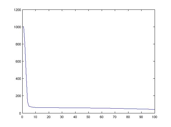
We start with a simple random example programmed in Matlab. Let $U_{0}$ be a random matrix in $\mathbb{R}^{50\times 8}$ with i.i.d. components having the uniform distribution on $[0,1]$. Let $V_{0}$ be a random matrix in $\mathbb{R}^{70\times 8}$ with components having the same distribution. Take $M=U_{0}V_{0}^{t}$, $\rho=100$, and random initial matrices. Figure 1 shows that the method converges to $M$ in the sense that it produces a sequence of matrices $U^{(k)}$ and $V^{(k)}$ whose product $U^{(k)}V^{(k)^{t}}$ converges to $M$.

Figure 1. Evolution of the error $M-U^{(k)}V^{(k)^{t}}$ as $k$ goes from 1 to 100 on a random example.

3. The case of outliers and missing data

Let $\Omega$ denotes the set of couples $(i,j)$ for which an observation of $M_{i,j}$ is available. The matrix factorization problem can be addressed by considering the following optimization problem

(3.7) $$\min_{Y,S,U,V\geqslant 0}\ \frac{1}{2}\sum_{(i,j)\in\Omega}(Y_{i,j}-(UV^{t})_{i,j})^{2}+\lambda\left\|S\right\|_{1}$$

subject to

(3.8) $$M = Y+S,$$

with $\left\|S\right\|_{1}=\sum_{i,j}\left|S_{ij}\right|$, and $\lambda$ is a relaxation parameter whose value is discussed in Section 4.

3.1. The augmented Lagrange function

The Lagrange function $L(Y,S,U,V,\Lambda)$ for our problem is equal to:

(3.9) $$\frac{1}{2}\sum_{(i,j)\in\Omega}(Y_{i,j}-(UV^{t})_{i,j})^{2}+\lambda\left\|S\right\|_{1}+\sum_{(i,j)\in\Omega}{\Lambda_{ij}(M_{ij}-Y_{ij}-S_{ij})}.$$

In order to enforce the constraint $M_{ij}=Y_{ij}-S_{ij}$ for all $(i,j)\in\Omega$, we introduce the following augmented Lagrange function

(3.10) $$L^{aug}(Y,S,U,V,\Lambda) = L(Y,S,U,V)+\rho\ \frac{1}{2}\sum_{(i,j)\in\Omega}{(M_{ij}-Y_{ij}-S_{ij})^{2}}.$$

We now introduce an Alternating Direction Method of Multipliers. This method consists of solving iteratively in all the variables one after the other, and then updating the dual variable. For this purpose, we compute in the next subsections the optimum value for the problem of minimizing the augmented Lagrange function with respect to each variable.

3.2. Individual minimization subproblems in $Y$, $S$, $U$, and $V$

3.2.1. Minimization with respect to $Y$.

The problem reduces to minimizing the function of the variable $Y$ given by

$$\frac{1}{2}\sum_{i,j}({Y_{ij}-(UV^{t})_{ij}})^{2}+\sum_{(i,j)\in\Omega}{\Lambda_{ij}(M_{ij}-Y_{ij}-S_{ij})}+\rho\frac{1}{2}\sum_{(i,j)\in\Omega}{(M_{ij}-Y_{ij}-S_{ij})^{2}}$$

Let us denote by $Y^{*}$ a solution to this problem. We have to consider two cases separately: either $(i,j)\in\Omega$, or $(i,j)\notin\Omega$. The case $(i,j)\notin\Omega$ is obvious, since it is straightforward to check that $Y_{ij}^{*}=(UV^{t})_{ij}$ is a solution. Setting the partial derivative to zero gives the result of the case $(i,j)\in\Omega$. To summarize, we obtain

(3.11) $$Y_{ij}^{*} = \begin{cases}\frac{1}{1+\rho}((UV^{t})_{ij}+\Lambda_{ij}+\rho(M_{ij}-S_{ij})),\ \textrm{ if}(i,j)\in\Omega,\\ \\ (UV^{t})_{ij}\textrm{ otherwise}.\end{cases}$$

3.2.2. Minimization with respect to $S$.

We have to minimize the function of $S$ given by

(3.12) $$\lambda\left\|S\right\|_{1}+\sum_{(i,j)\in\Omega}{\Lambda_{ij}(M_{ij}-Y_{ij}-S_{ij})}+\rho\frac{1}{2}\sum_{(i,j)\in\Omega}{(M_{ij}-Y_{ij}-S_{ij})^{2}}.$$

This can be performed by optimizing each component of $S$ independently of the other. As for the case of minimizing with respect to $Y$, we distinguish between two cases, while if $(i,j)\notin\Omega$ one easily checks that $S_{ij}^{*}=0$. If $(i,j)\in\Omega$, we will use the following result.

Theorem 3.1.

The solution to

(3.13) $$\min_{x\in\mathbb{R}}\frac{1}{2}(y-x)^{2}+\lambda\left|x\right|$$

is given by

(3.14) $$x^{*} = \begin{cases}y-\lambda\quad if\quad y>\lambda,\\ y+\lambda\quad if\quad y<\lambda,\\ 0\quad otherwise.\\ \end{cases}$$

Based on this result, we easily obtain

(3.15) $$S_{ij}^{*} = \begin{cases}-M_{ij}+Y_{ij}+\Lambda_{ij}-\frac{\lambda}{\rho},if-M_{ij}+Y_{ij}+\Lambda_{ij}>\frac{\lambda}{\rho},\\ -M_{ij}+Y_{ij}+\Lambda_{ij}+\frac{\lambda}{\rho},if-M_{ij}+Y_{ij}+\Lambda_{ij}<\frac{\lambda}{\rho},\\ 0\quad\textrm{ otherwise.}\end{cases}$$

3.2.3. Minimization with respect to $U$ and $V$.

We just have to use the fixed point subroutine given by (2.6).

3.3. Our Bregman proximal-type ADMM

We will choose the starting values as follows. Set $U^{(0)}$, $V^{(0)}$, $\Lambda^{(0)}$, $S^{(0)}=0$. Set

$$Y_{ij}^{0} = \begin{cases}M_{ij},\ \forall(i,j)\in\Omega,\\ \textrm{ imputation by the mean over all other observed values row $i$},\forall(i,j)\notin\Omega.\end{cases}$$

The Bregman-Proximal point ADMM is then given by

1. Set $S=S^{(k)},U=U^{(k)},V=V^{(k)},\Lambda=\Lambda^{(k)}$ and obtain $Y^{(k+1)}=Y^{*}$ given by (3.11),

2. Set $Y=Y^{(k+1)},U=U^{(k)},V=V^{(k)},\Lambda=\Lambda^{(k)}$ and obtain $S^{(k+1)}=S^{*}$ given by (3.15),

3. Set $Y=Y^{(k+1)},S=S^{(k+1)},U=U^{(k)},\Lambda=\lambda^{(k)}$ and obtain $U^{(k+1)}$ using the fixed point method (2.6)

4. Set $Y=Y^{(k+1)},S=S^{(k+1)},U=U^{(k+1)},\Lambda=\Lambda^{(k)}$ and obtain $U^{(k+1)}$ using the fixed point method (2.6).

5. Set $\Lambda^{(k+1)}=\Lambda^{(k)}+M-Y-S$

4. Choosing the $\lambda$ value

The choice of the parameter $\lambda$ is crucial for the good performances of the proposed method. We performed a selection of $\lambda$ using the following approach.

1. Propose an a priori range of values for $\lambda$ such that its maximum values leads to $S$ equals the null matrix at optimality.

2. For each value of $\lambda$, select a set $\mathcal{S}$ of $s$ entries chosen uniformly at random in $M$ and consider them as missing data temporarily.

   1. Find the solution of (3.7), where the missing data incorporate the set of entries which were artificially declared as missing in the previous step.

   2. Compute the average squared error on the data artificially declared as missing. Denote this quantity by $err_{\lambda}$.

3. Select $\lambda$ in the prescribed range as the one which minimizes the average squared error $err_{\lambda}$.

5. Application to bladder cancer expression data

5.1. Description of the data

The number of new patients affected by bladder cancer in 2013 attained 10,000 in France, thus improving the diagnosis of bladder cancer is a Public Health priority. Determining the genes responsible for bladder cancer would undoubtedly permit to design an efficient and adapted set of medical treatments.

First of all the treatment should depend on the advancement of the tumor. For this purpose, researchers have gathered important gene expression data and the corresponding state of the malignant tumor in the bladder of 100 patients in the Lyon region (France). This study concerns 34 selected genes and the tumor state was discretized into 4 classes.

From the statistical perspective, the data can be analyzed using PCA, cluster analysis, and polytomic logistic regression. Our approach in this section is to use Non-negative Matrix Factorization in order to jointly take into account the data’s intrinsic non-negative nature and the necessity of clustering the data by performing efficient feature extraction. One of the main challenges in the study of such data sets is to take into account possible outliers. For the bladder cancer dataset, some outliers have been observed by using standard PCA visualization, thus enforcing the need to automatically detect such phenomena in order to avoid subsequent misinterpretations of the genes’ respective influences on the tumor state.

The data array consists of one first column providing the tumor state. The next 34 columns provide the expression of 34 genes. The array has 100 lines which correspond to the number of patients. There are two principal classes of tumors:

• $TVNIM$ : noninfiltrating tumors;

• $TVIM$ : infiltrating tumors.

The tumor states have been classified into the following groups:

• $Ta$ : noninfiltrating tumor in Urothelium;

• $T1a$ : noninfiltrating tumor in Urothelium and parts of the chorion;

• $T1b$ : noninfiltrating tumor in Urothelium and the full chorion;

• $>T1$ : infiltrating tumor.

In the standard classification, the last group of the list incorporates states $T2$ to $T4b$.

5.2. Experimental results

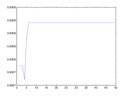
The ADMM algorithm was run on the experimental data. The choice of $\lambda$ was obtained using the strategy described in Section 4. The result obtained by this strategy is depicted in Figure 2.

Figure 2. The average squared prediction error on the artificially declared as missing entries as a function of $\lambda$

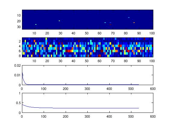
Based on the optimal choice of $\lambda$, the algorithm performances and the estimation results are depicted in Figure 3 and Figure 4.

The first subplot of Figure 3 represents the matrix $S$ after convergence, while the second subplot is the matrix $V^{t}$. The third subplot, for its part, represents the distance in Frobenius norm between two successive iterates of $\Lambda$. Finally, the fourth subplot represents the evolution of the relative error between $M$ and its NMF $U^{(k)}V^{(k)^{t}}$.

Figure 3. The factorization and convergence curves. The first subplot is $S$ after convergence. The second subplot is $V^{t}$. The third subplot, shows the distance between two successive iterates of $\Lambda$. The fourth subplot shows the relative error between $M$ and its NMF $U^{(k)}V^{(k)^{t}}$ as a function of iteration number

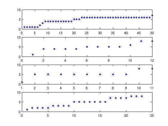
Figure 4 shows the cluster index in each subgroup "pTa", "pT1a", "pT1b", and "more serious than pT1" (i.e., ">pT1"). We see a sort of continuous drift in these cluster indices from pTa to >pT1. Indeed,

• pTa mostly consists of 3 subgroups indexed by $\{1,4,6\}$;

• pT1a mostly consists of 3 subgroups indexed by $\{4,5\}$;

• pT1b mostly consists of only one group, which is $\{5\}$;

• finally, >pT1 mostly consists of 5 subgroups indexed by $\{2,3,5,7,8\}$.

The intersection of the index subsets between two adjacent states is always a singleton, up to a discarded minority of individuals. The cluster indexed by 5 appears at medium to serious levels. The lowest level is characterized by cluster 6 while the most serious level is characterized by the more significant appearance of clusters 2,3,7, and 8.

Some more precise investigations should now be performed in order to understand the biological meaning of these clusters, i.e., to understand the factors of gravity in this cancer.

Figure 4. Cluster index for each group of patients. Subplot 1 corresponds to pTa, subplot 2 to pT1a, subplot 3 to pT1b, and subplot 4 to > pT1.

6. Conclusion

In this article, a new way to find a relevant dictionary for extracting the relevant features in a given dataset has been presented, in an original context of missing values and outliers. The well-known Non-negative Matrix Factorization (NMF) method has been extended on denoised data, where missing values have been guessed and outliers have been detected, leading to a mixture of Bregman proximal methods and the of Augmented Lagrangian scheme. Finally, an application to the analysis of gene expression data of patients with bladder cancer has been provided for illustration purpose.

7. Acknowledgements

The first and second authors were funded by the grant Eléments Transposables from the Région Franche-Comté. The first author would like to acknowledge the help of Haokun Li for the preparation of the manuscript. P. Huetz acknowledges the Montbelliard and Besançon Leagues against Cancer for financial support.

References

- [1] Berry, Michael W. and Browne, Murray, Email Surveillance Using Non-negative Matrix Factorization, Computational and Mathematical Organization Theory 11, (2005), no. 3 249–264.
- [2] Victor Bittorf, Benjamin Recht, C. Ré, and Joel A. Tropp, Factoring non-negative matrices with linear programs, NIPS 2012.
- [3] S. Bubeck, Theory of convex optimization for machine learning, http://www.princeton.edu/ sbubeck/Bubeck14.pdf.
- [4] E. J. Candès, X. Li, Y. Ma, and J. Wright, Robust Principal Component Analysis ? Journal of ACM 58, (2010), no.1, 1-37.
- [5] Chan, T.H., Ma, W.K., Chi, C.Y., Wang, Y.: A convex analysis framework for blind separation of non-negative sources. IEEE Trans. on Signal Processing, 56 (2008) no.10, 5120–5134.
- [6] Inderjit S. Dhillon, Suvrit Sra, Generalized Non-negative Matrix Approximations with Bregman Divergences, NIPS 2005.
- [7] Esser, E., Moller, M., Osher, S., Sapiro, G., Xin, J., A convex model for non-negative matrix factorization and dimensionality reduction on physical space. IEEE Trans. on Image Processing 21 (2012) no.7, 3239–3252.
- [8] Gillis, N. and Vavasis, S., Fast and robust recursive algorithms for separable non-negative matrix factorization, IEEE Trans. Pattern Anal. Mach. Intell. (2013).
- [9] https://sites.google.com/site/godecomposition/home.
- [10] Guillamet, D., Vitrià, J., Non-negative matrix factorization for face recognition. Lecture Notes in Artificial Intelligence, (2002), p. 336–344. Springer.
- [11] Jia, S. and Qian, Y., Constrained non-negative matrix factorization for hyperspectral unmixing. IEEE Trans. on Geoscience and Remote Sensing 47, (1), p. 161–173 (2009).
- [12] Hyunsoo Kim and Haesun Park, Sparse non-negative matrix factorizations via alternating non-negativity-constrained least squares for microarray data analysis, Bioinformatics 23, (2007), no. 12 1495–1502.
- [13] Daniel D. Lee and H. Sebastian Seung. Learning the parts of objects by non-negative matrix factorization, Nature 401 (1999), no. 6755, p. 788–791.
- [14] Li, Y., Sima, D., Van Cauter, S., Croitor Sava, A., Himmelreich, U., Pi, Y., Van Huffel, S., Hierarchical non-negative matrix factorization (hNMF): a tissue pattern differentiation method for glioblastoma multiforme diagnosis using MRSI. NMR in Biomedicine 26(3), 307–319 (2013).
- [15] Li, L., Lebanon, G. and Park, H., Fast Bregman divergence NMF using Taylor expansion and coordinate descent. Proc. of the 18th ACM SIGKDD Int. Conf. on Knowledge Discovery and Data Mining, pp. 307–315 (2012).
- [16] N. Parikh and S. Boyd Proximal Algorithms, Foundations and Trends in Optimization, 1(3):123-231, 2014.
- [17] Wei Xu, Xin Liu and Yihong Gong, Document clustering based on non-negative matrix factorization, "Proceedings of the 26th annual international ACM SIGIR conference on Research and development in information retrieval". New York: Association for Computing Machinery (2003), p. 267–273.