The quantum statistical parton distributions approach proposed more than one decade ago is revisited by considering a larger set of recent and accurate Deep Inelastic Scattering experimental results. It enables us to improve the description of the data by means of a new determination of the parton distributions. This global next-to-leading order QCD analysis leads to a good description of several structure functions, involving unpolarized parton distributions and helicity distributions, in a broad range of $x$ and $Q^{2}$ and in terms of a rather small number of free parameters. There are several challenging issues and in particular the confirmation of a large positive gluon helicity distribution. The predictions of this theoretical approach will be tested for single-jet production and charge asymmetry in $W^{\pm}$ production in $\bar{p}p$ and $pp$ collisions up to LHC energies, using recent data and also for forthcoming experimental results.

Key words: Deep inelastic scattering, Statistical distributions, Helicity asymmetries

PACS numbers: 12.40.Ee, 13.60.Hb, 13.88.+e, 14.70.Dj

1 Introduction

Deep Inelastic Scattering (DIS) of leptons and nucleons is indeed our main source of information to study the internal nucleon structure in terms of parton distributions. Several years ago a new set of parton distribution functions (PDF) was constructed in the framework of a statistical approach of the nucleon [1]. For quarks (antiquarks), the building blocks are the helicity dependent distributions $q^{\pm}(x)$ ($\bar{q}^{\pm}(x)$). This allows to describe simultaneously the unpolarized distributions $q(x)=q^{+}(x)+q^{-}(x)$ and the helicity distributions $\Delta q(x)=q^{+}(x)-q^{-}(x)$ (similarly for antiquarks). At the initial energy scale $Q_{0}^{2}$, these distributions are given by the sum of two terms, a quasi Fermi-Dirac function and a helicity independent diffractive contribution. The flavor asymmetry for the light sea, i.e. $\bar{d}(x)>\bar{u}(x)$, observed in the data is built in. This is simply understood in terms of the Pauli exclusion principle, based on the fact that the proton contains two up-quarks and only one down-quark. We predict that $\bar{d}(x)/\bar{u}(x)$ must remain above one for all $x$ values and this is a real challenge for our approach, in particular in the large $x$ region which is under experimental investigation at the moment. The flattening out of the ratio $d(x)/u(x)$ in the high $x$ region, predicted by the statistical approach, is another interesting challenge worth mentioning. The chiral properties of QCD lead to strong relations between $q(x)$ and $\bar{q}(x)$. For example, it is found that the well established result $\Delta u(x)>0$ implies $\Delta\bar{u}(x)>0$ and similarly $\Delta d(x)<0$ leads to $\Delta\bar{d}(x)<0$. This earlier prediction was confirmed by recent polarized DIS data and it was also demonstrated that the magnitude predicted by the statistical approach is compatible with recent BNL-RHIC data on $W^{\pm}$ production (see Section 5). In addition we found the approximate equality of the flavor asymmetries, namely $\bar{d}(x)-\bar{u}(x)\sim\Delta\bar{u}(x)-\Delta\bar{d}(x)$. Concerning the gluon, the unpolarized distribution $G(x,Q_{0}^{2})$ is given in terms of a quasi Bose-Einstein function, with only one free parameter, and for simplicity, we were assuming zero gluon polarization, i.e. $\Delta G(x,Q_{0}^{2})=0$, at the initial energy scale. As we will see below, the new analysis of a larger set of recent accurate DIS data, has forced us to give up this assumption. It leads to the confirmation of a large positive gluon helicity distribution, giving a significant contribution to the proton spin, a major point which was emphasized in a recent letter [2]. In our previous analysis all unpolarized and helicity light quark distributions were depending upon eight free parameters, which were determined in 2002 (see Ref. [1]), from a next-to-leading (NLO) fit of a small set of accurate DIS data. Concerning the strange quarks and antiquarks distributions, the statistical approach was applied using slightly different expressions, with four additional parameters [3]. Since the first determination of the free parameters, new tests against experimental (unpolarized and polarized) data turned out to be very satisfactory, in particular in hadronic reactions, as reported in Refs. [4, 5, 6].
It is crucial to note that the quantum-statistical approach differs from the usual global parton fitting methodology for the following reasons:
i) It incorporates physical principles to reduce the number of free parameters which have a physical interpretation
ii) It has very specific predictions, so far confirmed by the data
iii) It is an attempt to reach a more physical picture on our knowledge of the nucleon structure, the ultimate goal would be to solve the problem of confinement
iv) Treating simultaneously unpolarized distributions and helicity distributions, a unique siuation in the literature, has the advantage to give access to a vast set of experimental data, in particular up to LHC energies
The paper is organized as follows. In Section 2, we review the main points of our approach and we describe our method to determine the free parameters of the PDF with the set of experimental data we have used. In Section 3, we exhibit all the unpolarized and helicity distributions we have obtained. In Section 4, we show the results obtained for the unpolarized DIS structure functions $F_{2}^{p,d}(x,Q^{2})$ in a wide kinematic range, compared with the world data. We also consider $e^{\pm}p$ neutral and charged current reactions, and $\nu(\bar{\nu})p$ charged current reactions. This will be completed by our analysis of polarized DIS experiments, like double helicity asymmetries on a proton and on a neutron target. In Section 5, we present predictions for cross sections and helicity asymmetries in hadronic collisions, in particular inclusive single-jet production and $W$ production in $\bar{p}p$ and $pp$ collisions, up to LHC energies. We give our final remarks and conclusions in the last section.

2 Basic review on the statistical parton distributions

Let us now recall the main features of the statistical approach for building up the PDF, as opposed to the standard polynomial type parameterizations of the PDF, based on Regge theory at low $x$ and on counting rules at large $x$. The fermion distributions are given by the sum of two terms, a quasi Fermi-Dirac function and a helicity independent diffractive contribution:

$$xq^{h}(x,Q^{2}_{0})=\frac{A_{q}X^{h}_{0q}x^{b_{q}}}{\exp[(x-X^{h}_{0q})/\bar{x}]+1}+\frac{\tilde{A}_{q}x^{\tilde{b}_{q}}}{\exp(x/\bar{x})+1}~{},$$ (1)

$$x\bar{q}^{h}(x,Q^{2}_{0})=\frac{{\bar{A}_{q}}(X^{-h}_{0q})^{-1}x^{\bar{b}_{q}}}{\exp[(x+X^{-h}_{0q})/\bar{x}]+1}+\frac{\tilde{A}_{q}x^{\tilde{b}_{q}}}{\exp(x/\bar{x})+1}~{},$$ (2)

at the input energy scale $Q_{0}^{2}=1\mbox{GeV}^{2}$. We note that the diffractive term is absent in the quark helicity distribution $\Delta q$ and in the quark valence contribution $q-\bar{q}$.
In Eqs. (1,2) the multiplicative factors $X^{h}_{0q}$ and $(X^{-h}_{0q})^{-1}$ in the numerators of the non-diffractive parts of the $q$’s and $\bar{q}$’s distributions, imply a modification of the quantum statistical form, we were led to propose in order to agree with experimental data. The presence of these multiplicative factors was justified in our earlier attempt to generate the transverse momentum dependence (TMD) [7], which was revisited recently [8]. The parameter $\bar{x}$ plays the role of a universal temperature and $X^{\pm}_{0q}$ are the two thermodynamical potentials of the quark $q$, with helicity $h=\pm$. They represent the fundamental characteristics of the model. Notice the change of sign of the potentials and helicity for the antiquarks .
For a given flavor $q$ the corresponding quark and antiquark distributions involve the free parameters, $X^{\pm}_{0q}$, $A_{q}$, $\bar{A}_{q}$, $\tilde{A}_{q}$, $b_{q}$, $\bar{b}_{q}$ and $\tilde{b}_{q}$, whose number is reduced to $\it seven$ by the valence sum rule, $\int(q(x)-\bar{q}(x))dx=N_{q}$, where $N_{q}=2,1,0~{}~{}\mbox{for}~{}~{}u,d,s$, respectively.

For the light quarks $q=u,d$, the total number of free parameters is reduced to $\it eight$ by taking, as in Ref. [1], $A_{u}=A_{d}$, $\bar{A}_{u}=\bar{A}_{d}$, $\tilde{A}_{u}=\tilde{A}_{d}$, $b_{u}=b_{d}$, $\bar{b}_{u}=\bar{b}_{d}$ and $\tilde{b}_{u}=\tilde{b}_{d}$. For the strange quark and antiquark distributions, the simple choice made in Ref. [1] was improved in Ref. [3], but here they are expressed in terms of $\it seven$ free parameters.
For the gluons we consider the black-body inspired expression

$$xG(x,Q^{2}_{0})=\frac{A_{G}x^{b_{G}}}{\exp(x/\bar{x})-1}~{},$$ (3)

a quasi Bose-Einstein function, with $b_{G}$ being the only free parameter, since $A_{G}$ is determined by the momentum sum rule. In our earlier works [1, 5], we were assuming that, at the input energy scale, the polarized gluon, distribution vanishes, so

$$x\Delta G(x,Q^{2}_{0})=0~{}.$$ (4)

However as a result of the present analysis of a much larger set of very accurate unpolarized and polarized DIS data, we must give up this simplifying assumption. We are now taking

$$x\Delta G(x,Q^{2}_{0})=\frac{\tilde{A}_{G}x^{\tilde{b}_{G}}}{(1+c_{G}x^{d_{G}})}\!\cdot\!\frac{1}{\exp(x/\bar{x}-1)}\,.$$ (5)

It is clear that we don’t have a serious justification of the functional form of $\Delta G(x,Q^{2}_{0})$. However the above expression shows that it is strongly related to $G(x,Q^{2}_{0})$ and therefore constructed by means of a Bose-Einstein distribution with zero potential. Actually since $\Delta G(x,Q^{2}_{0})=P(x)G(x,Q^{2}_{0})$ a simpler expression would be $P(x)=Ax^{b}$, but the additional term $x^{d_{G}}$ in the denominator is needed in order to get a reasonable fit of the polarized DIS data. To insure that positivity is satisfied we must have $|P(x)|\leq 1$ (see section 3). However for quarks and antiquarks positivity is automatically fullfied by construction.
To summarize the new determination of all PDF’s involves a total of twenty one free parameters: in addition to the temperature $\bar{x}$ and the exponent $b_{G}$ of the gluon distribution, we have eight free parameters for the light quarks $(u,d)$, seven free parameters for the strange quarks and four free parameters for the gluon helicity distribution. These parameters will be determined from a next-to-leading order (NLO) QCD fit of a large set of accurate DIS data, unpolarized and polarized structure functions, as we will discuss in the following section.

3 Unpolarized and polarized parton distributions

In order to determine these parameters we have performed a global NLO QCD fitting procedure using only DIS data, because it is well known that the consideration of semi-inclusive DIS data involves uncertainties related to fragmentation functions. For unpolarized DIS we have considered $F_{2}^{p,d}(x,Q^{2})$ from NMC, E665, H1, ZEUS, neutral and charged current $e^{\pm}p$ cross sections from HERA and charged current neutrino and anti-neutrino cross sections from CCFR, NuTeV and CHORUS, which allow to extract $xF_{3}^{\nu N}(x,Q^{2})$. We present in Table 1 the details of the number of points and corresponding $\chi^{2}$ for each experiment, with a total of 1773 data points for a total $\chi^{2}$ of 2288.
For polarized DIS we have considered $g_{1}^{p,d,n}(x,Q^{2})$ from HERMES, E155, SMC, EMC, E143, E154, JLab and COMPASS. We present in Table 2 the details of the number of points and corresponding $\chi^{2}$ for each experiment, with a total of 269 data points for a total $\chi^{2}$ of 319.
The PDF QCD evolution was done in the $\overline{\bar{\mbox{MS}}}$ scheme using the HOPPET program [37], the minimization of the $\chi^{2}$ was performed with the CERN MINUIT program [38]. For unpolarized and polarized data we work in the General Mass Variable Flavour Number Scheme (GM-VFNS) [40, 41] and for the heavy quark we have taken $m_{c}$=1.275 GeV. For the strong running coupling $\alpha_{s}(Q^{2})$ we took $\alpha_{s}(Q^{2}_{0})=0.32$ and we find $\alpha_{s}(M_{z}^{2})=0.119\pm 0.001$. In our calculations $\alpha_{s}(M_{Z}^{2})$ is not a free parameter, it comes from the the evolution equations with an initial value $\alpha_{s}(Q_{0}^{2})=0.32$. For polarized data we have not introduced additional constraints coming from the hyperon decay constants, but we predict at $Q^{2}=2\mbox{GeV}^{2}$, F + D = 1.23 $\pm$ 0.03 and 3F - D = 0.57 $\pm$ 0.02, to be compared respectively with the experimental values $1.269\pm 0.003$ and $0.586\pm 0.031$ [42][43]. Concerning nuclear corrections for data involving nuclear targets, in the case of polarized data for $g_{1}^{d}$, we have taken into account the correction due to D-wave. For unpolarized data, there is an effect for $F_{2}$ only in the high $x$ region [39] that we have not considered. However for neutrino DIS data on iron target, the ratio of proton over neutron is included. For the kinematic cuts we have used the values given by the experiments and we have restricted the data to $Q^{2}>1\mbox{GeV}^{2}$ and $x>10^{-4}$. We are aware that target mass corrections can be included to improve the data description [39], but in this simple approach they were not considered. Also we have taken only leading-twist effects. The error bands were calculated using the standard Hessian matrix method, following the prescription described in Ref. [40] and we have used the standard choice of tolerance $\Delta\chi^{2}$ =1.

process	$\chi^{2}$	$N_{data}$	$\chi^{2}$/d.o.f.	$\chi^{2}$ 2002
$d\sigma$ ($\nu~{}p$) CCFR [9]	271	172	1.57	*410
$d\sigma$ ($\nu~{}p$) NuTeV [10]	206	177	1.16	*390
$d\sigma$ ($\nu~{}p$) CHORUS [11]	78	64	1.22	*176
$d\sigma$ ($\bar{\nu}~{}p$) CCFR [9]	191	163	1.17	*318
$d\sigma$ ($\bar{\nu}~{}p$) NuTeV [10]	153	125	1.22	*266
$F_{2}^{p}$ E665 [12]	24	11	2.18	17
$F_{2}^{p}$ ZEUS [13]	26	17	1.53	26
$F_{2}^{p}$ H1 [14, 15]	105	70	1.5	*292
$F_{2}^{p}$ NMC [16]	12	14	0.85	13
$F_{2}^{d}$ NMC [16]	230	155	1.48	274
$F_{2}^{d}/F_{2}^{p}$ NMC [17]	259	205	1.48	198
$F_{2}^{p}-F_{2}^{n}$ NMC [18, 19]	17	9	1.88	49
$xF_{3}^{\nu N}$ CHORUS [11]	65	47	1.38	*89
$xF_{3}^{\nu N}$ NuTeV [10]	68	49	1.38	100
Charged current $e^{+}p$ HERA [20]	33	32	1.03	*75
Charged current $e^{-}p$ HERA[20]	18	31	0.58	*24
Neutral current $e^{+}p$ HERA [20]	343	285	1.20	*520
Neutral current $e^{-}p$ HERA[20]	185	138	1.34	*383
$F_{L}$ H1 [21]	5	9	0.56	*37
Total	2288	1773

Table 1: Detailed $\chi^{2}$ for the cross sections and the unpolarized structure functions. In the column $\chi^{2}$ 2002 the values marked with an asterisk were not fitted in 2002.

process	$\chi^{2}$	$N_{data}$	$\chi^{2}$/d.o.f.	$\chi^{2}$ 2002
$g_{1}^{p}$ HERMES [22]	34	34	1	*36
$g_{1}^{p}$ E155 [23]	6	8	0.75	8
$g_{1}^{p}$ SMC [24]	25	12	2.08	35
$g_{1}^{p}$ EMC [26, 27]	9	10	0.9	8
$g_{1}^{p}$ E143 [28]	33	28	1.18	34
$g_{1}^{p}$ COMPASS [29]	16	9	1.77	*23
$g_{1}^{n}$ SMC [24]	4	7	0.57	8
$g_{1}^{n}$ E155 [23]	10	11	0.91	12
$g_{1}^{n}$ E154 [30]	5	11	0.45	6
$g_{1}^{n}$ E143 [28]	41	27	1.52	43
$g_{1}^{n}$ Jlab [31]	3	3	1	*1
$g_{1}^{d}$ HERMES [22, 34]	43	36	1.19	*70
$g_{1}^{d}$ COMPASS [35]	12	10	1.2	*30
$g_{1}^{d}$ E155 [36]	21	23	0.91	*43
$g_{1}^{d}$ E143 [28]	34	28	1.21	43
$g_{1}^{d}$ SMC [24]	23	12	1.92	*37
Total	319	269

Table 2: Detailed $\chi^{2}$ for the polarized structure functions $g_{1}^{p,d,n}(x,Q^{2})$. In the column $\chi^{2}$ 2002 the values marked with an asterisk were not fitted in 2002.

The new determination of the PDF leads, for the light quarks $(q=u,d)$, to the following parameters:

$$A_{q}=1.943\pm 0.005,~{}b_{q}=0.471\pm 0.001~{}\bar{A}_{q}=8.915\pm 0.050,$$

$${}~{}\bar{b}_{q}=1.301\pm 0.004,~{}\tilde{A}_{q}=0.147\pm 0.003,~{}\tilde{b}_{q}=0.0431\pm 0.003$$ (6)

and four potentials

$$X_{0u}^{+}=0.475\pm 0.001,~{}X_{0u}^{-}=0.307\pm 0.001,$$

$$X_{0d}^{+}=0.245\pm 0.001,~{}X_{0d}^{-}=0.309\pm 0.001.$$ (7)

Concerning the strange quarks we have the following parameters:

$$A_{s}=28.508\pm 0.005,~{}b_{s}=0.370\pm 0.002,~{}\bar{A}_{s}=0.0026\pm 0.0002,$$

$$\bar{b}_{s}=0.201\pm 0.003,~{}\tilde{A}_{s}=13.689\pm 0.050,~{}\tilde{b}_{s}=9.065\pm 0.020,$$ (8)

and two potentials

$$X_{0s}^{+}=0.011\pm 0.001,~{}X_{0s}^{-}=0.015\pm 0.001.$$ (9)

Finally in the gluon sector, we obtain the following parameters:

$$A_{G}=36.778\pm 0.085,~{}b_{G}=1.020\pm 0.0014,~{}\tilde{A}_{G}=26.887\pm 0.050,$$

$$\tilde{b}_{G}=0.163\pm 0.005,~{}c_{G}=0.006\pm 0.0005,~{}d_{G}=-6.072\pm 0.350.$$ (10)

In addition the new universal temperature is $\bar{x}=0.090\pm 0.002$.

By comparing with the results of 2002 [1], we have observed a remarkable stability of some important parameters, the light quarks potentials $X_{0u}^{\pm}$ and $X_{0d}^{\pm}$, whose numerical values are almost unchanged . The new temperature is slightly lower. As a result the main features of the new light quark and antiquark distributions are only scarcely modified. However it is instructive to note that in Tables 1 and 2, one can judge the improvement obtained in this new version compared to the old 2002 version. The last column gives the $\chi^{2}$ obtained with the old parameters and the new data set.
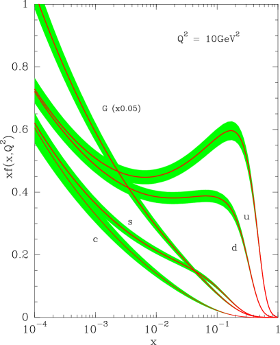
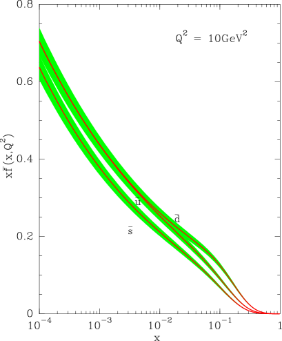
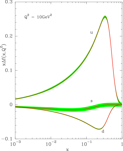
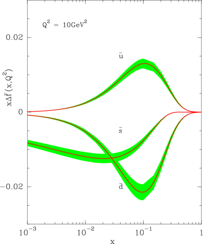
We display in Fig.1 the different unpolarized parton distributions $xf(x,Q^{2})$ ($f=u,d,s,c,\bar{u},\bar{d},\bar{s}~{}\mbox{and}{}~{}G$) versus $x$, after NLO QCD evolution at $Q^{2}=10\mbox{GeV}^{2}$ , with the corresponding error bands. Similarly the different quark and antiquark helicity distributions $x\Delta f(x,Q^{2})$ ($f=u,d,s,\bar{u},\bar{d}~{}\mbox{and}~{}\bar{s}$) versus $x$, after NLO QCD evolution at $Q^{2}=10\mbox{GeV}^{2}$ , with the corresponding error bands are shown in Fig. 2.
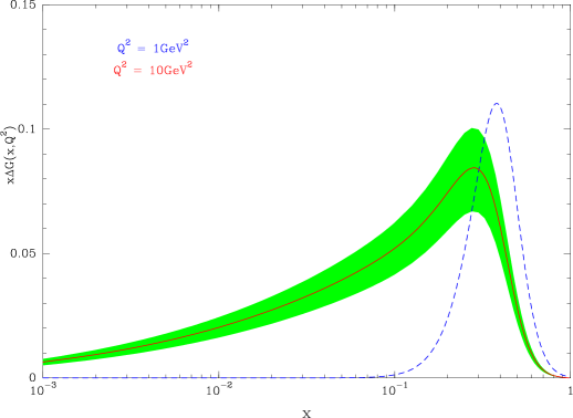
Our determination of the gluon helicity distribution deserves a special discussion. We display in Fig. 3Top the gluon helicity distribution versus $x$ at the initial scale $Q_{0}^{2}=1\mbox{GeV}^{2}$ and $Q^{2}=10\mbox{GeV}^{2}$. At the initial scale it is sharply peaked around $x=0.4$, but this feature lessens after some QCD evolution. We note that $P(x)$ introduced above, has the following expression, $P(x)=0.731x^{5.210}/(x^{6.072}+0.006)$, which is such that $0<P(x)<1$ for $0<x<1$, so positivity is satisfied and the gluon helicity distribution remains positive. As already mentioned the term $x^{d_{G}}$ plays an important role. It has a strong effect on the quality of the fit of $g_{1}^{p,n,d}(x,Q\textasciidieresis^{2})$, since the $\chi^{2}$ increases substantially when $d_{G}$ decreases. Its value also affects the shape of the gluon helicity distribution, which becomes larger towards the smaller $x$-values, for smaller $d_{G}$. We display $\Delta G(x,Q^{2})/G(x,Q^{2})$ in Fig. 3Bottom for two $Q^{2}$ values and some data points [44, 45], which suggest that the gluon helicity distribution is positive indeed. According to the constraints of the counting rules this ratio should go to 1 when $x=1$, but we observe that this is not the case here, since for example at the initial scale $P(x=1)=0.726$. In some other parameterizations in the current literature, this ratio goes to zero, since the large $x$ behavior of $x\Delta G(x)$ is $(1-x)^{\beta}$, with $\beta>>3$ [46, 47]. Clearly one needs a better knowledge of $\Delta G(x,Q^{2})/G(x,Q^{2})$ for $x>0.2$.

Figure 1: The different unpolarized parton distributions $xf(x,Q^{2})$ ($f=u,d,s,c,\bar{u},\bar{d},\bar{s}~{}\mbox{and}~{}G$) versus $x$, after NLO QCD evolution at $Q^{2}=10\mbox{GeV}^{2}$, with the corresponding error bands. The charm distributions $xc(x,Q^{2})=x\bar{c}(x,Q^{2})$ are generated by QCD evolution.

Figure 2: The different quark and antiquark helicity distributions $x\Delta f(x,Q^{2})$ ($f=u,d,s,\bar{u},\bar{d}~{}\mbox{and}~{}\bar{s}$) versus $x$, after NLO QCD evolution at $Q^{2}=10\mbox{GeV}^{2}$, with the corresponding error bands. The charm helicity distributions generated by QCD evolution are essentially zero

Figure 3: Top : The gluon helicity distribution $x\Delta G(x,Q^{2})$ versus $x$, for $Q^{2}=1~{}\mbox{GeV}^{2}$ (dashed curve) and after NLO QCD evolution for $Q^{2}=10~{}\mbox{GeV}^{2}$ (solid curve), with the corresponding error band .
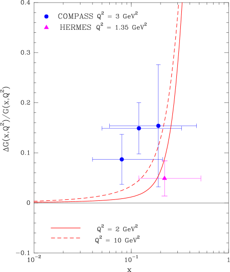
Bottom : $\Delta G(x,Q^{2})/G(x,Q^{2})$ versus $x$, for $Q^{2}=2~{}\mbox{GeV}^{2}$ (solid curve) and $Q^{2}=10~{}\mbox{GeV}^{2}$ (dashed curve). The data are from HERMES [44] and COMPASS [45]

4 Deep inelastic scattering

4.1 Unpolarized DIS experiments

First we present some selected experimental tests for the unpolarized PDF by considering $\mu N$ and $eN$ DIS, for which several experiments have yielded a large number of data points on the structure functions $F_{2}^{N}(x,Q^{2})$, $N$ stands for either a proton or a deuterium target. We have used fixed target measurements which probe a rather limited kinematic region in $Q^{2}$ and $x$ and also HERA data which cover a very large $Q^{2}$ range and probe the very low $x$ region, dominated by a fast rising behavior, consistent with our diffractive term (See Eq. (1)).
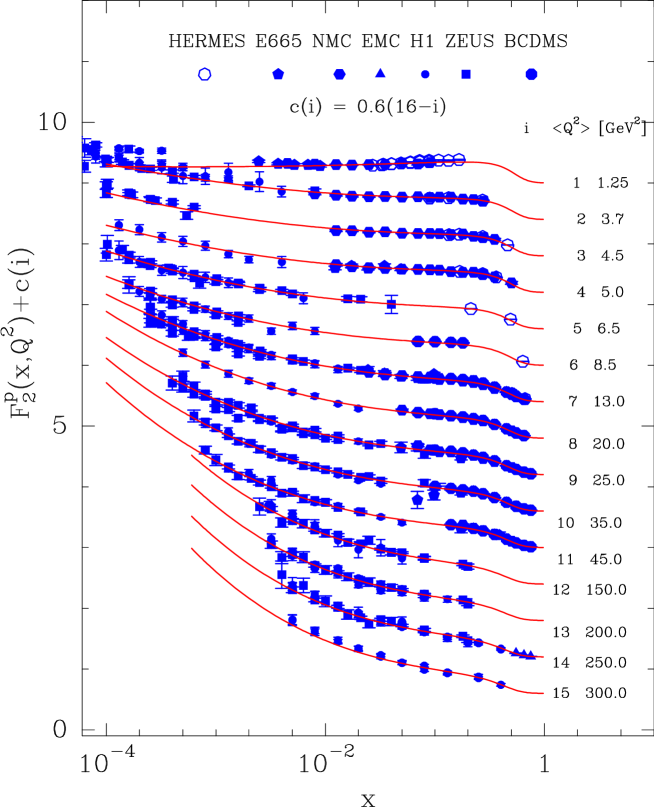
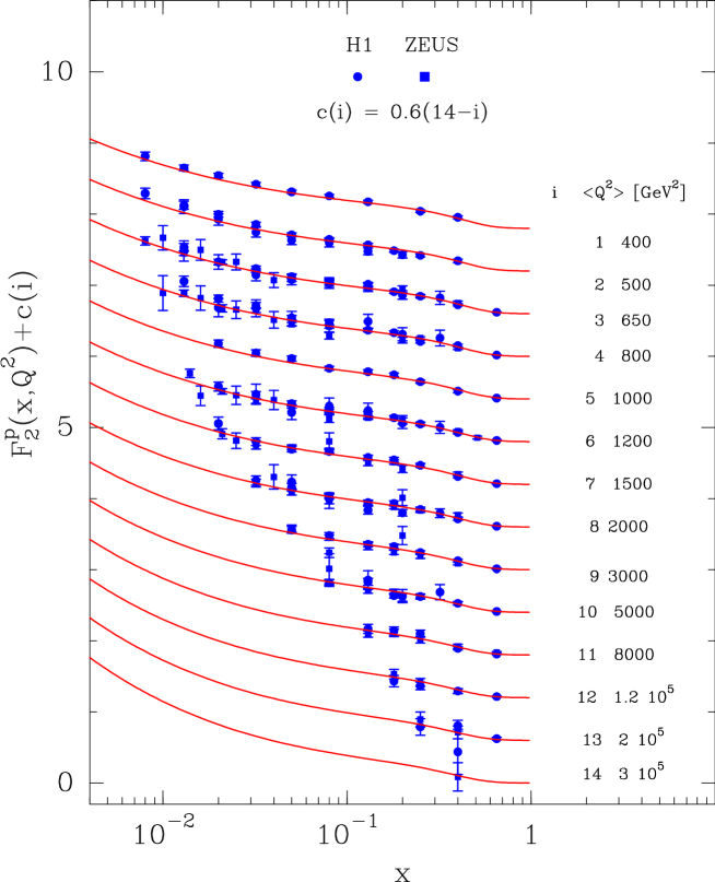
For illustration of the quality of our fit and, as an example, we show in Fig. 4 and Fig. 5, our results for $F_{2}^{p}(x,Q^{2})$ on different fixed proton targets, together with H1 and ZEUS data . We note that the analysis of the scaling violations leads to a gluon distribution $xG(x,Q^{2})$, in fairly good agreement with our simple parametrization (See Eq. (3)).

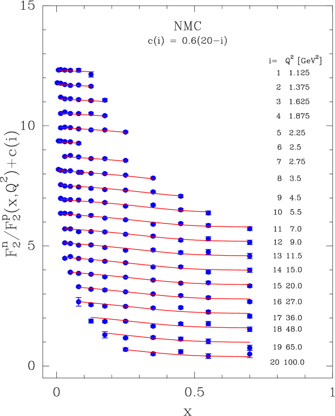
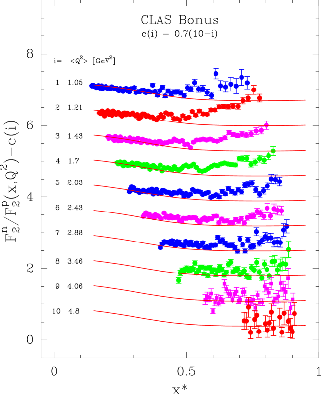
Another rather interesting physical quantity is the neutron $F_{2}^{n}$ structure function and in particular the ratio $F_{2}^{n}/F_{2}^{p}(x,Q^{2})$ which provides strong contraints on the PDF of the nucleon. For example the behavior of this ratio at large $x$ is directly related to the ratio of the $d$ to $u$ quarks in the limit $x\to 1$, a long-standing problem for the proton structure. We show the results of two experiments, NMC in Fig. 6, which is very accurate and covers a reasonable $Q^{2}$ range up to $x=0.7$ and CLAS in Fig.  7, which covers a smaller $Q^{2}$ range up to larger $x$ values, both are fairly well described by the statistical approach. Several comments are in order. In the small $x$ region this ratio, for both cases, tends to 1 because the structure functions are dominated by sea quarks driven by our universal diffractive term. In the high $x$ region dominated by valence quarks, the NMC data suggest that this ratio goes to a value of the order of 0.4 for $x$ near 1, which corresponds to the value 0.16 for $d(x)/u(x)$ when $x\to 1$, as found in the statistical approach [5]. The CLAS data at large $x$ cover the resonance region of the cross section and an important question is whether Bloom-Gilman duality holds as well for the neutron as it does for the proton. We notice that the predictions of the statistical approach suggest an approximate validity of this duality, except for some low $Q^{2}$ values. A better precision and the extension of this experiment with the 12GeV Jefferson Lab will certainly provide even stronger constraints on PDFs up to $x\simeq 0.8$.

Figure 4: $F^{p}_{2}(x,Q^{2})$ as a function of $x$ for fixed $\langle Q^{2}\rangle$ and data from HERMES [48], E665 [12], NMC [17], EMC [49], H1 [14, 15], ZEUS [13], BCDMS [50]. The function $c(i)=0.6(16-i)$, $i=1$ corresponds to $\langle Q^{2}\rangle=1.25\mbox{GeV}^{2}$ . The curves are the results of the statistical approach.

Figure 5: $F^{p}_{2}(x,Q^{2})$ as a function of $x$ for fixed high $\langle Q^{2}\rangle$ and data from H1 [14, 15], ZEUS [13]. The function $c(i)=0.6(14-i)$, $i=1$ corresponds to $\langle Q^{2}\rangle=400\mbox{GeV}^{2}$ . The curves are the results of the statistical approach.

Figure 6: $F^{n}_{2}/F^{p}_{2}(x,Q^{2})$ as a function of $x$ for fixed $\langle Q^{2}\rangle$ and data from NMC [51]. The function $c(i)=0.6(20-i)$, $i=1$ corresponds to $\langle Q^{2}\rangle=1.125\mbox{GeV}^{2}$. The curves are the results of the statistical approach.

Figure 7: $F^{n}_{2}/F^{p}_{2}(x,Q^{2})$ as a function of $x^{*}\simeq x$ (for the exact definition of $x^{*}$ see Ref. [52]) for fixed $\langle Q^{2}\rangle$ and data from CLAS BoNus [52]. The function $c(i)=0.7(10-i)$, $i=1$ corresponds to $\langle Q^{2}\rangle=1.05\mbox{GeV}^{2}$. The curves are the results of the statistical approach

We now turn to the inclusive neutral and charged current $e^{\pm}p$ cross sections which, in addition to $F_{2}^{p}$, give access to other structure functions.
The neutral current DIS processes have been measured at HERA in a kinematic region where both the $\gamma$ and the $Z$ exchanges must be considered. The cross sections for neutral current can be written, at lowest order, as

$$\frac{d^{2}\sigma^{\pm}_{NC}}{dxdQ^{2}}=\frac{2\pi\alpha^{2}}{xQ^{4}}\left[Y_{+}\tilde{F}_{2}(x,Q^{2})\mp Y_{-}x\tilde{F}_{3}(x,Q^{2})-y^{2}F_{L}(x,Q^{2})\right]~{},$$ (11)

where

$$\tilde{F}_{2}(x,Q^{2})\!\!=\!\!F_{2}^{\gamma}(x,Q^{2})-v_{e}\chi_{z}(Q^{2})F_{2}^{\gamma Z}(x,Q^{2})+\!\!(a_{e}^{2}+v_{e}^{2})\chi^{2}_{z}(Q^{2})F_{2}^{Z}(x,Q^{2})~{},$$ (12)

$$x\tilde{F}_{3}(x,Q^{2})=-a_{e}\chi_{z}(Q^{2})xF_{3}^{\gamma Z}(x,Q^{2})+2a_{e}v_{e}\chi^{2}_{z}(Q^{2})xF_{3}^{Z}(x,Q^{2})~{}.$$ (13)

The structure function $F_{L}(x,Q^{2})$ is sizeable only at high $y$ and we will come back to it later. The other structure functions introduced above, have the following expressions in terms of the parton distributions

$$\left[F_{2}^{\gamma},F_{2}^{\gamma Z},F_{2}^{Z}\right](x,Q^{2}) = \sum_{f}\left[e^{2}_{f},2e_{f}v_{f},a^{2}_{f}+v^{2}_{f}\right]\left(xq_{f}(x,Q^{2})+x\bar{q}_{f}(x,Q^{2})\right),$$

$$\left[xF_{3}^{\gamma Z},xF_{3}^{Z}\right](x,Q^{2}) = \sum_{f}\left[2e_{f}a_{f},2a_{f}v_{f}\right]\left(xq_{f}(x,Q^{2})-x\bar{q}_{f}(x,Q^{2})\right).$$ (14)

Here the kinematic variables are $y=Q^{2}/xs$, $Y_{\pm}=1\pm(1-y)^{2}$, $\sqrt{s}=2\sqrt{E_{e}E_{p}}$, $E_{e}$ and $E_{p}$ are the electron (positron) and proton beam energies respectively. Morever, $v_{i}$ and $a_{i}$ are the vector and axial-vector weak coupling constants for the lepton $e$ and the quark $f$, respectively, and $e_{f}$ is the charge. The function $\chi_{z}(Q^{2})$ is given by

$$\chi_{z}(Q^{2})=\frac{1}{\sin^{2}{2\theta_{W}}}\frac{Q^{2}}{Q^{2}+M^{2}_{Z}}~{},$$ (15)

where $\theta_{W}$ is the weak mixing angle and $M_{Z}$ is the $Z$-boson mass. The reduced cross sections are defined as

$$\tilde{\sigma}^{\pm}_{NC}(x,Q^{2})=\frac{Q^{4}x}{Y_{+}2\pi\alpha^{2}}\frac{d^{2}\sigma^{\pm}_{NC}}{dxdQ^{2}}~{}.$$ (16)

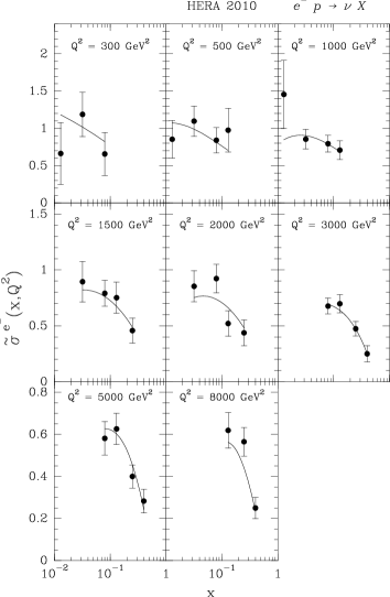
Our predictions are compared with HERA data in Fig. 8, as a function of $x$, in a broad range of $Q^{2}$ values and the agreement is good.

Figure 8: Top : Comparison of the data on the reduced neutral cross section $\tilde{\sigma}^{NC}(x,Q^{2})$, in $e^{-}p$ collisions as a function of $x$ and for different $Q^{2}$ values, with the results of the statistical approach. Data are from HERA [20].
Bottom : Same for $e^{+}p$ collisions.

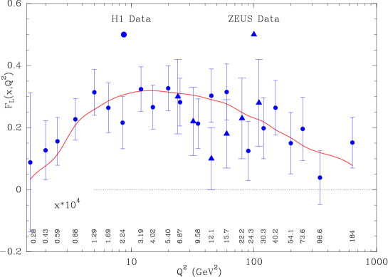
For low $Q^{2}$, the contribution of the longitudinal structure function $F_{L}(x,Q^{2})$. to the cross section at HERA is only sizeable at $x$ smaller than approximately $10^{-3}$ and in this domain the gluon density dominates over the sea quark density. More precisely, it was shown that [54]

$$F_{L}(x,Q^{2}) = \frac{\alpha_{s}(Q^{2})}{\pi}\left[\frac{4}{3}\int_{x}^{1}\frac{dy}{y}(\frac{x}{y})^{2}F_{2}(y,Q^{2})\right.$$ (17)

$$\left.+2\Sigma_{i}e_{i}^{2}\int_{x}^{1}\frac{dy}{y}(\frac{x}{y})^{2}(1-\frac{x}{y})yG(y,Q^{2})\right]$$

Before HERA was shut down, a dedicated run period, with reduced proton beam energy, was approved, allowing H1 to collect new results on $F_{L}$. We show on Fig. 9 the expectations of the statistical approach compared to the new data, whose precision is reasonable. The trend and the magnitude of the prediction are in fair agreement with the data, so this is another test of the good predictive power of our theoretical framework.

Figure 9: The longitudinal proton structure function $F_{L}(x,Q^{2})$ averaged in $x$ at given $Q^{2}$ values. Data are from ZEUS [55] and H1 [56] and the curve is the result of the statistical approach.

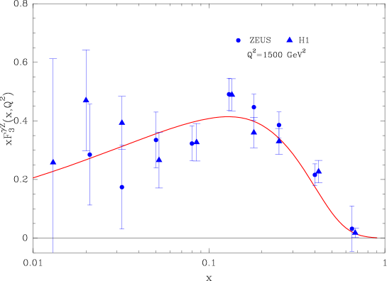
One can also test the behavior of the interference term between the photon and the $Z$ exchanges, which can be isolated in neutral current $e^{\pm}p$ collisions at high $Q^{2}$. We have to a good approximation, if sea quarks are ignored, $xF_{3}^{\gamma Z}(x,Q^{2})=\frac{x}{3}(2u_{v}+d_{v})(x,Q^{2})$ and comparison between data and prediction is shown in Fig. 10.

Figure 10: The interference term $xF_{3}^{\gamma Z}$ extracted in $e^{\pm}p$ collisions at HERA. Data are from ZEUS [57] and H1 [58], the curve is the prediction of the statistical approach.

The charged current DIS processes have been also measured accurately at HERA in an extented kinematic region. It has a serious impact on the determination of the unpolarized parton distributions by allowing a flavor separation because they involve only the $W^{\pm}$ exchange. The cross sections are expressed, at lowest order, in terms of three structure functions as follows

$$\frac{d^{2}\sigma^{e^{\pm}}_{Born}}{dxdQ^{2}} = \frac{G_{F}^{2}}{4\pi}\frac{M^{4}_{W}}{(Q^{2}+M^{2}_{W})^{2}}\left[Y_{+}F^{cc}_{2}(x,Q^{2})-y^{2}F^{cc}_{L}(x,Q^{2})\right.$$ (18)

$$\left.{\mp}Y_{-}xF^{cc}_{3}(x,Q^{2})\right]~{},$$

and the reduced cross sections are defined as

$$\tilde{\sigma}^{e^{\pm}}(x,Q^{2})=\left[\frac{G_{F}^{2}}{4\pi}\frac{M^{4}_{W}}{(Q^{2}+M^{2}_{W})^{2}}\right]^{-1}\frac{d^{2}\sigma^{cc}}{dxdQ^{2}}~{}.$$ (19)

At leading order for $e^{-}p\rightarrow\nu_{e}X$ with a longitudinally polarized beam

$$F^{cc}_{2}(x,Q^{2}) = x[u(x,Q^{2})+c(x,Q^{2})+\bar{d}(x,Q^{2})+\bar{s}(x,Q^{2})]$$

$$xF^{cc}_{3}(x,Q^{2}) = x[u(x,Q^{2})+c(x,Q^{2})-\bar{d}(x,Q^{2})-\bar{s}(x,Q^{2})]~{},$$ (20)

and for $e^{+}p\rightarrow\bar{\nu}_{e}X$

$$F^{cc}_{2}(x,Q^{2}) = x[d(x,Q^{2})+s(x,Q^{2})+\bar{u}(x,Q^{2})+\bar{c}(x,Q^{2})]$$

$$xF^{cc}_{3}(x,Q^{2}) = x[d(x,Q^{2})+s(x,Q^{2})-\bar{u}(x,Q^{2})-\bar{c}(x,Q^{2})]~{}.$$ (21)

At NLO in QCD $F^{cc}_{L}$ is non zero, but it gives negligible contribution, except at $y$ values close to 1. Our predictions for $\sigma^{cc}(x,Q^{2})$ at NLO are compared with H1 and ZEUS data in Fig. 11, as a function of $x$ in a broad range of $Q^{2}$ values.
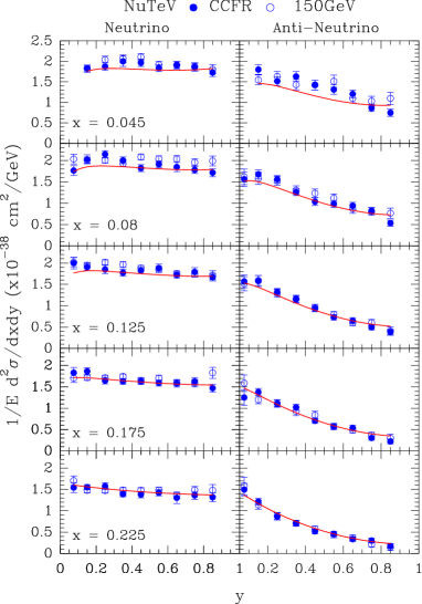
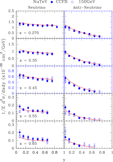
The differential inclusive neutrino and antineutrino cross sections have the following standard expressions

$$\frac{d^{2}\sigma^{\nu,(\bar{\nu})}}{dxdy} = \frac{G^{2}_{F}M_{p}E_{\nu}}{\pi(1+\frac{Q^{2}}{M^{2}_{W}})^{2}}\left[xy^{2}F_{1}^{\nu(\bar{\nu})}(x,Q^{2})+(1-y-\frac{M_{p}xy}{2E_{\nu}})F_{2}^{\nu(\bar{\nu})}(x,Q^{2})\right.$$ (22)

$$\left.\pm(y-\frac{y^{2}}{2})xF_{3}^{\nu(\bar{\nu})}(x,Q^{2})\right]\,,$$

$y$ is the fraction of total leptonic energy transfered to the hadronic system and $E_{\nu}$ is the incident neutrino energy. $F_{2}$ and $F_{3}$ are given by Eq. (20) for $\nu p$ and Eq. (21) for $\bar{\nu}p$, and $F_{1}$ is related to $F_{2}$ by

$$2xF_{1}=\frac{1+4x^{2}M^{2}_{p}/Q^{2}}{1+R}F_{2}\,,$$ (23)

where $R=\sigma_{L}/\sigma_{T}$, the ratio of the longitudinal to transverse cross sections of the W-boson production. Our results at NLO compared with the CCFR and NuTeV data are shown in Fig. 12. As expected, for fixed $x$, the $y$ dependence is rather flat for neutrino and has the characteristic $(1-y)^{2}$ behavior for antineutrino.

Figure 11: Left : Comparison of the data on the reduced charged cross section $\tilde{\sigma}^{e^{-}}(x,Q^{2})$, in $e^{-}p$ collisions as a function of $x$ and for different $Q^{2}$ values, with the results of the statistical approach. Data are from HERA [20].
Right : Same for $e^{+}p$ collisions.

Figure 12: Comparison of the data on the differential cross sections $\nu({\bar{\nu}})N$ for $E_{\nu}$ = 150 GeV, as a function of $y$ and for different $x$ values, with the results of the statistical approach. Data are from CCFR [9] and NuTeV [10].

4.2 Polarized DIS experiments

The spin-dependent structure function $g_{1}(x,Q^{2})$ has the well-known NLO QCD expression [59]

$$g_{1}(x,Q^{2}) = \frac{1}{2}\sum_{q}^{n_{f}}e_{q}^{2}[(\Delta q+\Delta\bar{q})\otimes(1+\frac{\alpha_{s}(Q^{2})}{2\pi}\delta C_{q})$$ (24)

$$+\frac{\alpha_{s}(Q^{2})}{2\pi}\Delta G\otimes\frac{\delta C_{G}}{n_{f}}],$$

$\Delta q(x,Q^{2}),\Delta\bar{q}(x,Q^{2})$ and $\Delta G(x,Q^{2})$ are quark, antiquark and gluon helicity distributions in the nucleon. $\delta C(x)_{q,G}$ are the NLO spin-dependent Wilson coefficient functions and the symbol $\otimes$ denotes the usual convolution in Bjorken $x$ space. $n_{f}$ is the number of active flavors for light quarks.
We recall that according to the results shown in Section 3, we have obtained a good flavor separation of these helicity distributions: for all $x$ and $Q^{2}$ values, $\Delta u>0$ is the largest one, $\Delta d<0$ is smaller in magnitude, $\Delta\bar{u}>0$ and $\Delta\bar{d}<0$ are approximately opposite and $\Delta s<0$, $\Delta\bar{s}<0$ are much smaller.

We now turn to the important issue concerning the asymmetries $A_{1}^{p,d,n}(x,Q^{2})$, measured in polarized DIS. We recall the definition of the asymmetry $A_{1}(x,Q^{2})$, namely

$$A_{1}(x,Q^{2})=\frac{[g_{1}(x,Q^{2})-\gamma^{2}(x,Q^{2})g_{2}(x,Q^{2})]}{F_{2}(x,Q^{2})}\frac{2x[1+R(x,Q^{2})]}{[1+\gamma^{2}(x,Q^{2})]}~{},$$ (25)

where $g_{1,2}(x,Q^{2})$ are the polarized structure functions, $\gamma^{2}(x,Q^{2})=4x^{2}M_{p}^{2}/Q^{2}$ and $R(x,Q^{2})$ is the ratio between the longitudinal and transverse photoabsorption cross sections. When $x\to 1$ for $Q^{2}=4~{}\mbox{GeV}^{2}$, $R$ is the order of 0.30 or less and $\gamma^{2}(x,Q^{2})$ is close to 1, so if the $u$ quark dominates, we have $A_{1}\sim 0.6\Delta u(x)/u(x)$, so it is unlikely to find $A_{1}\to 1$, as required by the counting rules prescription, which we don’t impose. We display in Fig. 13 the world data on $A_{1}^{p}(x,Q^{2})$ (Top) and $A_{1}^{n}(x,Q^{2})$ (Bottom), with the results of the statistical approach at $Q^{2}=4\mbox{GeV}^{2}$, up to $x=1$. Indeed we find that $A_{1}^{p,n}<1$.

Finally one important outcome of this new analysis of the polarized DIS data in the framework of the statistical approach, is the confirmation of a large positive gluon helicity distribution, which gives a significant contribution to the proton spin [2].

Figure 13: Top : Comparison of the world data on $A_{1}^{p}(x,Q^{2})$ with the result of the statistical approach at $Q^{2}=4~{}\mbox{GeV}^{2}$, including the corresponding error band.
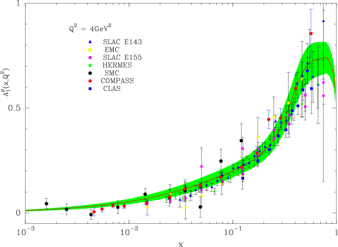
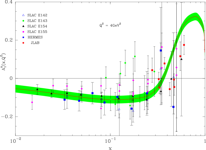
Bottom : Comparison of the world data on $A_{1}^{n}(x,Q^{2})$ with the result of the statistical approach at $Q^{2}=4~{}\mbox{GeV}^{2}$, including the corresponding error band. Data are from [22] - [33].

5 Hadronic collisions

A precise determination of parton distributions allows us to use them as input information to predict strong interaction processes, for additional tests of pertubative QCD and also for the search of new physics. Here we shall test our statistical parton distributions for the description of two inclusive reactions, single-jet and $W^{\pm}$ productions in $pp$ and $\bar{p}p$ collisions.

5.1 Single-jet production in $pp$ and $\bar{p}p$ collisions

The cross section for the production of a single-jet of rapidity $y$ and transverse momentum $p_{T}$, in a $pp$ or $\bar{p}p$ collision is given, at lowest-order (LO), by

$$E\frac{d^{3}\sigma}{dp^{3}} = \sum_{ij}\frac{1}{1+\delta_{ij}}\frac{2}{\pi}\int_{x_{0}}^{1}dx_{a}\frac{x_{a}x_{b}}{2x_{a}-x_{T}e^{y}}\times$$ (26)

$$\left[f_{i}(x_{a},Q^{2})f_{j}(x_{b},Q^{2})\frac{d\hat{\sigma}_{ij}}{d\hat{t}}(\hat{s},\hat{t},\hat{u})+(i\leftrightarrow j)\right]~{},$$

where $x_{T}=2p_{T}/\sqrt{s}$, $x_{0}=x_{T}e^{y}/(2-x_{T}e^{-y})$, $x_{b}=x_{a}x_{T}e^{-y}/(2x_{a}-x_{T}e^{y})$ and $\sqrt{s}$ is the center of mass energy of the collision. In the above sum, $i,j$ stand for initial gluon-gluon, quark-gluon and quark-quark scatterings, $d\hat{\sigma}_{ij}/d\hat{t}$ are the corresponding partonic cross sections and $Q^{2}$ is the scaling variable. The NLO QCD calculations were done using a code described in Ref. [60], based on a semi-analytical method within the ”small-cone approximation, improved recently with a jet anti-$k_{T}$ algorithm for a better definition [61] . In Fig. 14(Top) our results are compared with the data from STAR experiment at BNL-RHIC and this prediction agrees very well with the data.
Now we would like to test, in a pure hadronic collision, our new positive gluon helicity distribution, mentioned in Section 2. In a recent paper, the STAR experiment at BNL-RHIC has reported the observation, in single-jet inclusive production, of a non-vanishing positive double-helicity asymmetry $A_{LL}^{jet}$ for $5\leq p_{T}\leq 30$GeV, in the near-forward rapidity region [63]. We show in Fig. 14(Bottom) our prediction compared with these high-statistics data points and the agreement is very reasonable.

Figure 14: Top: Double-differential inclusive single-jet cross section in $pp$ collisions at $\sqrt{s}$ = 200GeV, versus $p_{T}^{jet}$, with jet radius parameter R=0.7, for $-0.8<\eta<0.8$, from STAR data, obtained with an integrated luminosity of 5.39pb^-1 [62] and the prediction from the statistical approach.
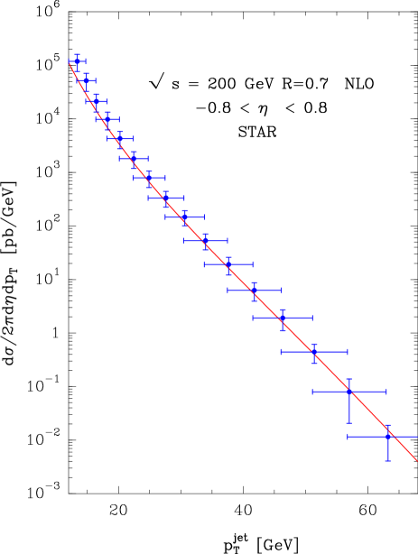
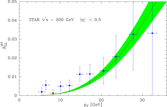
Bottom: Our predicted double-helicity asymmetry $A_{LL}^{jet}$ for single-jet production at BNL-RHIC in the near-forward rapidity region, versus $p_{T}$ and the data points from STAR [63], with the corresponding error band.

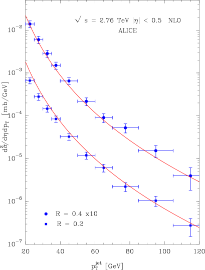
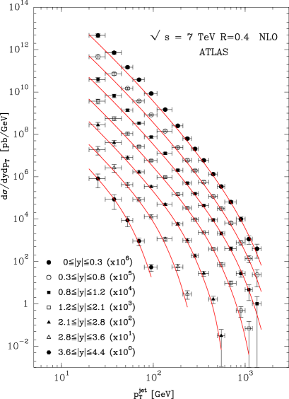
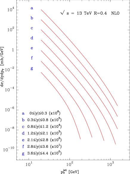
There are several data sets for the cross section of single-jet production which will allow us to test our predictions. First we show in Fig. 15(Top), the results, versus $p_{T}^{jet}$ for different rapidity bins, from D0 [64] and the results from ALICE [65] in Fig. 15(Bottom). Except ALICE, STAR and D0 are in good agreement with the statistical approach, as well as the results from ATLAS and CMS displayed in Fig. 16 at $\sqrt{s}$ = 7TeV. We are giving in Table 3 the detailed number of data points and $\chi^{2}$ for all these experiments. Given the fact that the experimental results are falling off over more than eight orders of magnitude, this is a remarkable confirmation of the Standard Model expectations, leaving no room for new physics. However some deviations might occur when LHC will reach a higher energy regime and this is why we give in Fig. 17, our predictions for the single-jet cross section at $\sqrt{s}$ = 13TeV.

Experiment	$\sqrt{s}$ TeV	$\chi^{2}$	$N_{data}$	$\chi^{2}$/d.o.f.
STAR [62]	0.2	11	16	0.67
D0 [64]	1.96	97	110	0.88
ALICE [65]	2.76	67	20	3.38
ATLAS [66]	7.0	127	88	1.45
CMS [67]	7.0	374	132	2.84

Table 3: Detailed $\chi^{2}$ prediction for the inclusive single jet production.

Figure 15: Top: Double-differential inclusive single-jet cross section in $\bar{p}p$ collisions at $\sqrt{s}$ = 1.96TeV, versus $p_{T}^{jet}$, with jet radius parameter R = 0.7, for different rapidity bins from D0 [64] and the predictions from the statistical approach Bottom: Same from ALICE [65] in $pp$ collisions at $\sqrt{s}$ = 2.76TeV, with R = 0.2, 0.4 and $|\eta|<0.5$.

Figure 16: Top: Double-differential inclusive single-jet cross section in $pp$ collisions at $\sqrt{s}$ = 7TeV, versus $p_{T}^{jet}$, with jet radius parameter R = 0.4, for different rapidity bins from ATLAS [66] and the predictions from the statistical approach
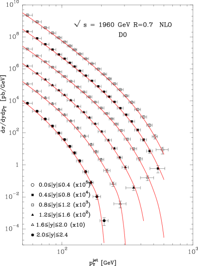
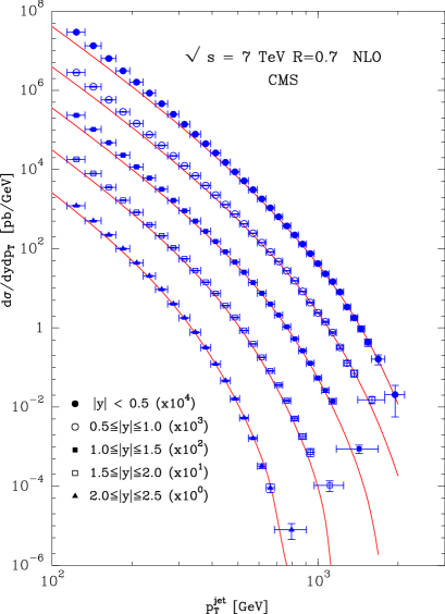
Bottom: Same from CMS [67], with R = 0.7.

Figure 17: Predicted cross sections for single-jet production in $pp$ collisions at $\sqrt{s}$ = 13TeV, versus $p_{T}^{jet}$, with jet radius parameter R = 0.4, for different rapidity bins.

5.2 $W^{\pm}$ production in $pp$ and $\bar{p}p$ collisions

Let us recall that for the $W^{\pm}$ production in $pp$ collision, the differential cross section $d\sigma_{pp}^{W^{\pm}}/dy$ can be computed directly from the Drell-Yan picture in terms of the dominant quark-antiquark fusion reactions $u\bar{d}\to W^{+}$ and $\bar{u}d\to W^{-}$. So for $W^{+}$ production, we have to LO

$$d\sigma_{pp}^{W^{+}}/dy\sim u(x_{1},M_{W}^{2})\bar{d}(x_{2},M_{W}^{2})+\bar{d}(x_{1},M_{W}^{2})u(x_{2},M_{W}^{2})~{},$$ (27)

where $x_{1,2}=M_{W}/\sqrt{s}\exp(\pm y)$, $y$ is the rapidity of the W and $\sqrt{s}$ denotes the $c.m.$ energy of the collision. For $W^{-}$ production, we have a similar expression, after quark flavors interchanged and clearly these $y$ distributions are symmetric under $y\to-y$. In the case of $\bar{p}p$ collision we have

$$d\sigma_{\bar{p}p}^{W^{+}}/dy\sim u(x_{1},M_{W}^{2})d(x_{2},M_{W}^{2})+\bar{d}(x_{1},M_{W}^{2})\bar{u}(x_{2},M_{W}^{2})~{},$$ (28)

which is no longer symmetric under $y\to-y$. However $W^{+}$ and $W^{-}$ production cross sections are simply related since we have $\frac{d\sigma_{\bar{p}p}^{W^{-}}}{dy}(y)=\frac{d\sigma_{\bar{p}p}^{W^{+}}}{dy}(-y)$.
Let us now turn to the charge asymmetry defined as

$$A(y)=\frac{\frac{d\sigma_{\bar{p}p}^{W^{+}}}{dy}(y)-\frac{d\sigma_{\bar{p}p}^{W^{-}}}{dy}(y)}{\frac{d\sigma_{\bar{p}p}^{W^{+}}}{dy}(y)+\frac{d\sigma_{\bar{p}p}^{W^{-}}}{dy}(y)}~{},$$ (29)

and clearly we have $A(y)=-A(-y)$.
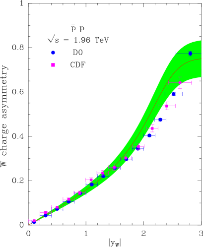
It contains very valuable informations on the light quarks distributions inside the proton and in particular on the ratio of down-to-up-quark, as noticed long time ago [68]. Although the cross sections are largely modified by NLO and NNLO QCD corrections, it turns out that these effects do not affect the LO calculation of the charge asymmetry [69]. A direct measurement of this asymmetry has been achieved at FNAL-Tevatron by CDF [70] and D0 [71] and the results are shown in Fig. 18, together with the prediction of the statistical approach. The agreement is very good in the low-$y$ region. However in the high-$y$ region the charge asymmetry might not flatten out, following the behavior of our predicted $d(x)/u(x)$ ratio in the high-$x$ region (see Fig. 4 of Ref. [5]).
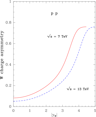
In view of forthcoming data from the LHC, we display in Fig. 19, predictions from the statistical approach at $\sqrt{s}$ = 7 and 13 TeV. In this case the $W$ charge asymmetry is symmetric in $y_{W}$ and at fixed $y_{W}$ it decreases for increasing energy.

Figure 18: The measured $W$ production charge asymmetry at FNAL-Tevatron [70, 71], versus the $W$ rapidity $y_{W}$ and the prediction from the statistical approach, including the corresponding error band.

Figure 19: The predictions from the statistical approach for the $W$ production charge asymmetry at the LHC energies, $7\mbox{TeV}$ (solid line) and $13\mbox{TeV}$ (dashed line), versus the $W$ rapidity $y_{W}$.

However, it is not always possible to reconstruct the $W$-boson and to measure the boson rapidity, because of the energy carried away by the neutrinos in leptonic $W$-boson decays. A quantity more directly accessible experimentally is the lepton charge asymmetry, defined as

$$A(\eta)=\frac{d\sigma/d\eta(W^{+}\to l^{+}\nu)-d\sigma/d\eta(W^{-}\to l^{-}\bar{\nu})}{d\sigma/d\eta(W^{+}\to l^{+}\nu)+d\sigma/d\eta(W^{-}\to l^{-}\bar{\nu})},$$ (30)

where $d\sigma/d\eta$ is the differential cross section for $W$-boson production and subsequent leptonic decay and $\eta=-\ln{[\tan{(\theta/2)}]}$ is the charged lepton pseudorapidity in the laboratory frame, with $\theta$ being the polar angle measured with respect to the beam axis.

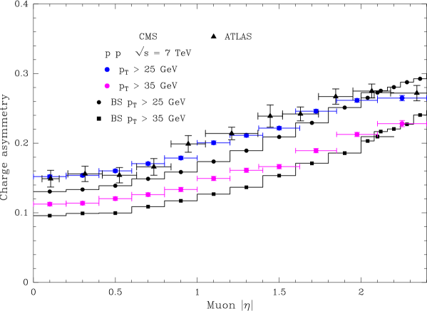
There was an earlier experimental result at the LHC from ATLAS [72], obtained with a total integrated luminosity of 31pb^-1, but more recently CMS [73] released a data sample corresponding to a total integrated luminosity of. 4.7fb^-1. We display in Fig. 20 both data sets, together with the results of our calculations, which were obtained using the FEWZ code [74]. Although the statistical approach is compatible with CMS data, a higher accuracy is required before considering that it is a very conclusive test of our PDF’s.

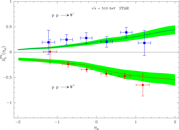
Finally we consider the process $\overrightarrow{p}p\to W^{\pm}+X\to e^{\pm}+X$, where the arrow denotes a longitudinally polarized proton and the outgoing $e^{\pm}$ have been produced by the leptonic decay of the $W^{\pm}$-boson. The parity-violating asymmetry is defined as

$$A_{L}^{PV}=\frac{d\sigma_{+}-d\sigma_{-}}{d\sigma_{+}+d\sigma_{-}}~{}.$$ (31)

Here $\sigma_{h}$ denotes the cross section where the initial proton has helicity $h$. It is an excellent tool for pinning down the quark helicity distributions, as first noticed in Ref. [75].

$A_{L}^{PV}$ was measured recently at RHIC-BNL [76] and the results are shown in Fig. 21. As explained in Ref. [6], the $W^{-}$ asymmetry is very sensitive to the sign and magnitude of $\Delta\bar{u}$, so this is another successful result of the statistical approach.

Figure 20: The $\mu$ charge asymmetry from $W$-boson decays in bins of absolute muon pseudorapidity at the LHC $7\mbox{TeV}$, with some kinematical cuts $p_{T}^{\mu}>$ 20GeV for ATLAS [72] and $p_{T}^{\mu}>$ 25, 35GeV for CMS [73] with the predictions of the statistical approach (BS).

Figure 21: The measured parity-violating helicity asymmetries $A_{L}^{PV}$ for charged-lepton production at BNL-RHIC from STAR [76], through production and decay of $W^{\pm}$-bosons versus $y_{e}$ the charged-lepton rapidity. The solid curves are the predictions of the statistical approach, including the error bands.

6 Concluding remarks

Our quantum statistical approach to parton distributions, proposed thirteen years ago, has been revisited in the light of a large set of most recent world data from spin-averaged and spin-dependent pure DIS experiments, excluding semi-inclusive DIS and hard scattering processes. The construction of the PDF allows us to obtain simultaneously the unpolarized distributions and the helicity distributions, a rather unique situation. In the current literature one finds, on the one hand, global QCD analysis of spin-averaged experiments, some including LHC data, [58, 77, 78, 79, 80, 81] to extract unpolarized distributions and, on the other hand, global QCD analysis of spin-dependent experiments [46, 47, 82, 83], to determine the helicity distributions. They don’t restrict themselves to DIS experiments, like we do, and in general their parameterizations involve many free parameters, whose total number and physical meaning are considered to be irrelevant.

Our aim in the analysis of the DIS data was to incorporate in the structure of the PDF some physical principles, like Bose-Einstein distributions for gluons and Fermi-Dirac distributions for quarks and antiquarks, which are simply related from chiral properties of QCD. This allows us to reduce the number of free parameters, some of them having a physical interpretation. The improvements we have obtained from this new version is a more accurate determination of light quarks, strange quarks, strongly related to their corresponding antiquarks, and gluon distributions. We have found a large positive gluon helicity distribution, $\Delta G(x,Q^{2})$, very similar to that coming from the results of Ref. [82] (see also Ref. [83]) and compatible with a new high energy hadron collider result. As we have seen there are several challenging questions related to large-$x$ predictions, because the large-$x$ structure of hadrons is essential for a complete picture.

The predictive power of our approach lies partly in the DIS sector, but mainly in the rich domain of hadronic collisions, up to LHC energies. We have shown that our predictions for several spin-averaged and spin-dependent processes at RHIC, Tevatron and LHC, are already in fair agreement with existing data and we expect this will be confirmed by forthcoming experiments.

References

- [1] C. Bourrely, F. Buccella and J. Soffer, Eur. Phys. J. C 23, 487 (2002)
- [2] C. Bourrely and J. Soffer, Phys. Lett. B 740, 168 (2015)
- [3] C. Bourrely, F. Buccella and J. Soffer, Phys. Lett. B 648, 39 (2007)
- [4] C. Bourrely, F. Buccella and J. Soffer, Mod. Phys. Lett. A 18, 771 (2003)
- [5] C. Bourrely, F. Buccella and J. Soffer, Eur. Phys. J. C 41, 327 (2005)
- [6] C. Bourrely, F. Buccella and J. Soffer, Phys. Lett. B 726, 296 (2013)
- [7] C. Bourrely, F. Buccella and J. Soffer, Phys. Rev. D 83, 074008 (2011)
- [8] C. Bourrely, F. Buccella and J. Soffer, Int. J. of Mod. Phys. A 28, 1350026 (2013)
- [9] U. K. Yang (CCFR/NuTeV Collaboration), Phys. Rev. Lett. 87, 251802 (2001)
- [10] M. Tzanov (NuTeV Collaboration), Phys. Rev. D 74, 012008 (2006)
- [11] G. Onengut (CHORUS Collaboration), Phys. Lett. B 632, 65 (2006)
- [12] R. Adams (E665 Collaboration), Phys. Rev. D 54, 3006 (1996)
- [13] S. Chekanov (ZEUS Collaboration), Eur. Phys. J. C 21, 443 (2001)
- [14] F.D. Aaron (H1 Collaboration), Eur. Phys. J. C 64, 561 (2009)
- [15] F.D. Aaron (H1 Collaboration), Eur. Phys. J. C 71, 1579 (2011)
- [16] M. Arneodo (NMC Collaboration) Nucl. Phys. B 483, 3 (1997)
- [17] M. Arneodo (NMC Collaboration), Nuc. Phys. B 487, 3 (1997)
- [18] P. Amaudruz (NMC Collaboration), Phys. Rev. Lett. 66, 2712 (1991)
- [19] M. Arneodo (NMC Collaboration), Phys. Rev. D 50, R1 (1994)
- [20] F.D. Aaron (H1 and ZEUS Collaborations), JHEP 1001, 109 (2010)
- [21] F.D. Aaron (H1 Collaboration), Eur. Phys. J. C 71, 1579 (2011)
- [22] A. Airapetian (HERMES Collaboration), Phys. Rev. D 71, 012003 (2005)
- [23] P.L Anthony (SLAC E155 Collaboration), Phys. Lett. B 493, 19 (2000)
- [24] B. Adeva (SMC Collaboration), Phys. Rev. D 58, 112001 (1998)
- [25] P. L. Anthony (SLAC E142 Collaboration), Phys. Rev. D 54, 6620 (1996)
- [26] J. Ashman (EMC Collaboration), Phys. Lett. B 206, 364 (1988)
- [27] J. Ashman (EMC Collaboration), Nucl. Phys. B 328, 1 (1989)
- [28] K. Abe (SLAC E143 Collaboration), Phys. Rev. D 58, 112003 (1998)
- [29] M.G. Alekseev (COMPASS Collaboration), Phys. Lett. B 690, 466 (2010)
- [30] K. Abe (SLAC E154 Collaboration), Phys. Rev. Lett. 79, 26 (1997)
- [31] X. Zheng (Jefferson Lab Hall A Collaboration), Phys. Rev. C 70, 065207 (2004)
- [32] D.S. Parno , Phys. Rev. C 91, 045506 (2015) arXiv:1406.1207 [nucl-ex]
- [33] K.V. Dharmawardane (CLAS Collaboration), Phys. Lett. B 641, 11 (2006)
- [34] A. Airapetian (HERMES Collaboration), Phys. Rev. D 75, 012007 (2007)
- [35] V.Yu. Alexakhin (COMPASS Collaboration), Phys. Lett. B 647, 8 (2007)
- [36] P.L. Anthony (SLAC E155 Collaboration), Phys. Lett. B 463, 339 (1999)
- [37] G.P. Salam and J. Rojo, Comput. Phys. Commun. 180, 120 (2009) (arXiv:0804.3755 [hep-ph])
- [38] F. James and M. Roos, CERN Program Library Long Writeup D506 (1994)
- [39] S. Alekhin, J. Blümlein and S. Moch, Phys. Rev. D 86, 054009 (2012) and references therein
- [40] A.D. Martin, W. J. Stirling, R. S. Thorne and G. Watt, Eur. Phys. J. C 63, 189 (2009)
- [41] R.S. Thorne, Phys. Rev. D 85, 054017 (2012)
- [42] K.A. Olive et al. (Particle Data Group) Chin. Phys. C 38, 090001 (2014)
- [43] A. Airapetian et al. (HERMES Collaboration), Phys. Rev. D 75, 012007 (2007) and Erratum ibid., D 76, 039901 (2007)
- [44] A. Airapetian et al. (HERMES Collaboration), JHEP 1008, 130 (2010)
- [45] M. Stolarski (COMPASS Collaboration), preliminary results presented at DIS 2014.
- [46] D. de Florian, R. Sassot, M. Stratmann and W. Vogelsang, Phys. Rev. Lett. 101, 072001 (2008); Phys. Rev. D 80, 034030 (2009)
- [47] R. D. Ball et al. (NNPDF Collaboration), Nucl. Phys. B 874, 36 (2013); J. Blümlein and H. Böttcher, Nucl. Phys. B 841, 205 (2010); E. Leader, A. V. Sidorov and D. B. Stamenov, Phys. Rev. D 83, 114018 (2010); M. Hirai and S. Kumano, Nucl. Phys. B 813, 106 (2009); P. Jimenez-Delgado, A. Accardi and W. Melnitchouk, Phys. Rev. D 89, 034025 (2014)
- [48] A. Airapetian et al. (HERMES Collaboration), JHEP 1105, 125 (2011)
- [49] J.J. Aubert et al. (EMC Collaboration), Nucl. Phys. B 259, 189 (1985)
- [50] A.C. Benvenuti et al. (BCDMS Collaboration), Phys. Lett. B 223, 485 (1989)
- [51] M. Arneodo et al. (NMC Collaboration), Nucl. Phys. B 371, 3 (1992)
- [52] N. Baillie et al. (CLAS Collaboration), Phys. Rev. Lett. 108, 142001 (2012), Erratum-ibid 108, 199902 (2012)
- [53] S. Moch and J.A.M. Vermaseren, Nucl. Phys. B 573, 853 (2000) and references therein
- [54] G. Altarelli and G. Martinelli, Phys. Lett. B 76, 89 (1978)
- [55] S. Chekanov et al. (ZEUS Collaboration), Phys. Lett. B 682, 8 (2009)
- [56] V. Andreev (H1 Collaboration), Eur. Phys. J. C 74, 2814 (2014)
- [57] H. Abramowicz et al. (ZEUS Collaboration), Phys. Rev. D 87, 052014 (2013)
- [58] F.D. Aaron (H1 Collaboration), JHEP 1209, 061 (2012)
- [59] W. Vogelsang, Phys. Rev. D 54, 2023 (1996)
- [60] B. Jager, M. Stratmann and W. Vogelsang, Phys. Rev. D 70, 034010 (2004)
- [61] A. Mukherjee and W. Vogelsang, Phys. Rev. D 86, 094009 (2012)
- [62] B. Abelev et al. (STAR Collaboration), Phys. Rev. Lett. 97, 252001 (2006); see also T. Sakuma, MIT Thesis (2009)
- [63] L. Adamczyk et al. (STAR Collaboration), arXiv:1405.5134 [hep-ex].
- [64] V.M. Abazov (D0 Collaboration), Phys. Rev. D 85, 052006 (2012)
- [65] B. Abelev et al. (ALICE Collaboration), Phys. Lett. B 722, 262 (2013)
- [66] G. Aad et al. (ATLAS Collaboration), arXiv:1410.8857 [hep-ex]
- [67] S. Chatrchyan (CMS Collaboration), Phys. Rev. D 87, 112002 (2013); Erratum-ibid, 119902
- [68] E.L. Berger, F. Halzen, C.S. Kim and S. Willenbrock, Phys. Rev. D 40, 83 (1989); Erratum-ibid 3789
- [69] Ch. Anastasiou, L. Dixon, K. Melnikov and F. Petriello, Phys. Rev. D 69, 094008 (2004)
- [70] T. Aaltonen et al. (CDF Collaboration), Phys. Rev. Lett. 102, 181801 (2009)
- [71] V.M. Abazov et al. (D0 Collaboration), Phys. Rev. Lett. 112, 151803 (2014)
- [72] G. Aad et al. (ATLAS Collaboration), Phys. Rev. 85, 072004 (2012)
- [73] S. Chatrchyan (CMS Collaboration), Phys. Rev. D 90, 032004 (2014)
- [74] R. Gavin et al., Comput. Phys. Commun. 182, 2388 (2011)
- [75] C. Bourrely and J. Soffer, Phys. Lett. B 314, 132 (1993)
- [76] L. Adamczyk et al. (STAR Collaboration), Phys. Rev. Lett. 113, 072301 (2014)
- [77] L.A. Harland-Lang, A.D. Martin, P. Motylinski and R.S. Thorne, arXiv:1412.3989v1 [hep-ph] and references therein
- [78] R.D. Ball et al. (NNPDF Collaboration) arXiv:1410.8849v2 [hep-ph]
- [79] H.L. Lai , Phys. Rev. D 82, 074024 (2010)
- [80] S. Alekhin, J. Blümlein and S. Moch, Phys. Rev. D 89, 054028 (2014) and references therein
- [81] P. Jimenez-Delgado and E. Reya, Phys. Rev. D 89, 074049 (2014)
- [82] D. de Florian, R. Sassot, M. Stratmann and W. Vogelsang, Phys. Rev. Lett. 113, 012001 (2014)
- [83] E. R. Nocera et al. (NNPDF Collaboration), arXiv:1406.5539v2 [hep-ph]