Why Is The Neutrino Oscillation Formula Expanded In $\Delta m_{21}^{2}/\Delta m_{31}^{2}$ Still Accurate Near The Solar Resonance In Matter?

Abstract

The conventional approximate formula for neutrino oscillation in matter which is obtained from the expansion in terms of the ratio of mass square differences $\alpha=\Delta m_{21}^{2}/\Delta m_{31}^{2}\approx 0.03$, first proposed by Cervera, et al and Freund, turns out to be an accurate formula for accelerator neutrino experiments. Originally it required the neutrino energy to be well above the solar resonance to validate the expansion but it is found to be still very accurate when the formula is extrapolated to the resonance, which is practically important for the T2K experiment. This paper shows that the accuracy is guaranteed by cancellations of branch cut singularities and also, for the first time, analytically computes the actual error of the formula. The actual error implies that the original requirement can be safely removed in current experiments.

1 Introduction

In long-baseline(LBL) neutrino experiments, the matter effectWolfenstein (1978); Mikheev and Smirnov (1985, 1986) is usually not negligible. For current LBL accelerator neutrino experiments such as T2KAbe et al. (2013a, 2014), MINOSAdamson et al. (2011) and NOvAAyres et al. (2004); Patterson (2013) where the matter densities are almost constant, there is a useful approximate formula for the transition probability. Taking the same notations as PDG, the formula isOlive et al. (2014)

$$P(\nu_{\mu}\rightarrow\nu_{e}) = 4s_{13}^{2}c_{13}^{2}s_{23}^{2}\frac{\sin^{2}(1-A)\Delta}{(1-A)^{2}}$$ (1)

$$+8\alpha\frac{J_{CP}}{s_{\delta}}\cos(\Delta+\delta)\frac{\sin A\Delta}{A}\frac{\sin(1-A)\Delta}{1-A}$$

$$+4\alpha^{2}s_{12}^{2}c_{12}^{2}c_{23}^{2}\frac{\sin^{2}A\Delta}{A^{2}}$$

where

$$A\equiv 2\sqrt{2}G_{F}N_{e}E/\Delta m_{31}^{2},\thinspace\alpha\equiv\Delta m_{21}^{2}/\Delta m_{31}^{2}\approx 0.03,$$ (2)

and $\Delta\equiv\Delta m_{31}^{2}L/(4E)$. $N_{e}$ is the electron number density in matter, about $1.4\textrm{cm}^{-3}N_{A}$ in the Earth’s crust.

The formula was originally derived in Cervera et al. (2000); Freund (2001) as a series expansion in $\alpha$. But the problem is that due to the non-perturbative behavior near the solar resonance, the expansion is expected to be valid only when the neutrino energy is well above the solar resonance,

$$E\gg 0.34\textrm{GeV}\frac{\Delta m_{21}^{2}}{7.6\times 10^{-5}\textrm{eV}^{2}}\frac{1.4\textrm{cm}^{-3}N_{A}}{N_{e}}.$$ (3)

This was emphasized in ref.Freund (2001), because the approximation $\alpha/A\ll 1$ was used when the formula was derived. We will reformulate the derivation of the formula in section 2 to show the problem more explicitly but here we take the solar mixing angle $\theta_{12}$ as a good example to show the problem. The effective $\sin 2\theta_{12}$ in matter, denoted as $\sin 2\theta_{12}^{m}$, expanded in $\alpha$ to first order, is Freund (2001)

$$\sin 2\theta_{12}^{m}\sim\alpha/A.$$ (4)

The solar resonance is at $A=\alpha\cos 2\theta_{12}\approx 0.4\alpha$ so near the solar resonance $\sin 2\theta_{12}^{m}$ is quite likely to be larger than 1. As will be shown in section 2, $\sin 2\theta_{12}^{m}>1$ does appear in the expansion when the energy is lower than $0.34\textrm{GeV}$, which makes the calculation invalid. Originally, $\sin 2\theta_{12}^{m}$ in the calculation was expected not only less than 1 but also small, i.e. $\sin 2\theta_{12}^{m}\ll 1$, otherwise the unitarity of the effective mixing matrix will be badly violated, thereby invalidating the calculation.

Despite the claimed bound (3) in Freund (2001), in practice this formula works well below the bound (see figures 6, 7 presented later in this paper). For example T2K has used this formula in their recent publicationAbe et al. (2013b) because eq.(1) exhibits excellent accuracy near the solar resonance .

So (3) is most likely not the true bound of validity. We would like to know to what extent the formula is accurate or valid. The main goal of this paper, is to mathematically demonstrate that there is no lower bound of $A$ for the domain of validity. We will provide explicit errors of the formula, among which the main error related to the matter effect is only $\mathcal{O}(s_{13}^{2}\alpha A\Delta^{2})$. This implies that the formula is still accurate when $A$ is close to $\alpha$ and one may apply (1) below the bound.

Note that a higher order calculation in the original perturbative approach will not work since the series in $\alpha/A$ can not converge at the resonance if the branch cut singularity is not treated carefully. Actually a higher order correction to the formula (1) is computed in ref.Asano and Minakata (2011) but the correction blows up when taking the vacuum limit $A\rightarrow 0$. Thus it can not give a correct estimation when $A$ is small. This is due to a lack of careful treatment of the branch cut singularity related to the solar resonance.

Branch cuts in the oscillation system with the matter effect are essentially related to level crossings Akhmedov et al. (2008); Blennow and Smirnov (2013), but less noticed before. Note that the three eigenvalues of the oscillation system come from the same cubic equation but they are different. The difference originates from the different branches in the square roots and cubic roots in the general solutions of a cubic equation. At a level crossing two of the eigenvalues are very close to each other which makes the problem quite non-perturbative and this just corresponds to the starting point of the branch cuts, which are called branch cut singularities. The branch cut singularities are essentially origins of all non-perturbativities in the oscillation system. In this paper, we will remove the singularity corresponding to the solar resonance in our analytic calculation by transformation of the eigenvalues to some singularity-free variables and compute the $S$-matrix using the Cayley-Hamilton theorem. In this way the conventional formula will be proven to be accurate below the bound (3). The relation between the branch cut singularities and level crossings will be discussed in detail and thus improve our understanding of the matter effect in neutrino oscillationAkhmedov et al. (2001, 2007); Xing (2013); Chiu et al. (2010); Takamura and Kimura (2006); Arafune et al. (1997); Blennow and Ohlsson (2005); Ohlsson and Winter (2003); Ohlsson et al. (2013); Schwetz (2007); Yokomakura et al. (2002); Smirnov (2014); Freund et al. (2000); Zhang (2007).

As a byproduct of our analysis, a new approximate formula is derived in this paper, with better accuracy. Though the exact form is a little more complicated than (1), for practical use in neutrino simulation, it is useful and covers most aspects. This is important considering that simulation of LBL experiments and performing $\chi^{2}$-fits require a fast and simple method to compute a large number of oscillation probabilities. Therefore even though the numerical calculation is always viable, there are still many studies on analytic approximation formulae for neutrino oscillation in matterAkhmedov et al. (2004); Honda et al. (2006); Agarwalla et al. (2014); Zhou (2011); Takamura et al. (2004, 2005); Harrison and Scott (2002); Kimura et al. (2002a, b); Ohlsson (2001); Yasuda (2014); Asano and Minakata (2011); Minakata and Parke (2015).

This paper is organized as follows. In section 2, we reformulate the original derivation of the formula (1) and numerically show the accuracy of the $\alpha$-expansion in the case of T2K. We will see that the $\alpha$-expansion for some effective parameters is actually invalid below $0.34\textrm{GeV}$ in T2K while the final result of the probability is very accurate. Then in section 3 from the viewpoint of singularities, we show that non-differentiable singularities in many parameters originate from the branch cut and result in the failure of the $\alpha$-expansion. In section 4 we solve the problem rigorously and then compute the analytical error of (1). Based on the calculation in section 4, we also propose an alternative to the conventional formula. Their accuracies are numerically verified, which will be shown in section 5. Finally we conclude in section 6.

2 The $\alpha$-expansion and the accidental accuracy

In this section, we first introduce analytic diagonalization of the $3\times 3$ effective Hamiltonian, which has early been done by Zaglauer and Schwarzer Zaglauer and Schwarzer (1988) without any approximation. Then we show the $\alpha$-expansion of the result from Freund’s calculationFreund (2001) and compare the approximate result with the exact result (though complicated but numerically programmable) to see how much it deviates from the exact result. We will show that the $\alpha$-expansion result of effective neutrino parameters are quite inaccurate and even invalid near the solar resonance but the final result (i.e. the assembled oscillation probability) from these parameters is very accurate.

Neutrino oscillation in matter is subjected to the Schrödinger equation in the flavor space,

$$i\frac{d}{dL}|\nu(L)\rangle=H|\nu(L)\rangle,$$ (5)

where $|\nu(L)\rangle$ denotes the flavor state of the evolving neutrino at a distance of $L$ from the source and $H$ is the Hamiltonian represented by the $3\times 3$ matrix in the standard neutrino oscillation framework,

$$H=\frac{1}{2E}U.\left(\begin{array}[]{ccc}m_{1}^{2}\\ &m_{2}^{2}\\ &&m_{3}^{2}\end{array}\right).U^{\dagger}+\sqrt{2}G_{F}N_{e}\left(\begin{array}[]{ccc}1\\ &0\\ &&0\end{array}\right).$$ (6)

Here $U$ and $m_{i}$’s are neutrino mixing matrix and masses in vacuum respectively. The second term in eq.(6) comes from the matter effect. Without the second term (i.e. $N_{e}=0$), the solution of (5) is quite simple since the first term has already been diagonalized. So in vacuum, the transition amplitude of $\nu_{\alpha}\rightarrow\nu_{\beta}$ is just

$$S_{\alpha\beta}=U_{\alpha 1}U_{\beta 1}^{*}+U_{\alpha 2}U_{\beta 2}^{*}e^{i\alpha\Delta}+U_{\alpha 3}U_{\beta 3}^{*}e^{i\Delta}.$$ (7)

Here $S_{\alpha\beta}$ is usually referred to as the $S$-matrix in neutrino oscillation. For neutrino oscillation in matter, we need to diagonalize (6) to obtain the effective mixing matrix $\tilde{U}$ and the effective neutrino masses $\tilde{m}_{k}$, defined as

$$H=\frac{1}{2E}\tilde{U}diag(\tilde{m}_{1}^{2},\tilde{m}_{2}^{2},\tilde{m}_{3}^{2})\tilde{U}^{\dagger}.$$ (8)

Then $\tilde{U}$ and $\tilde{m}_{k}$, combined in the way similar to (7), gives the $S$-matrix in matter.

The $3\times 3$ matrix $H$ can be analytically diagonalized by solving first the eigenvalues and then the corresponding eigenvectors, though the computation is complicated.

The process can be a little simplified if we extract a dimensionless matrix $M$ from

$$H=\frac{m_{1}^{2}}{2E}+\frac{\Delta m_{31}^{2}}{2E}M,$$ (9)

and define

$$M_{d}=U^{\dagger}MU.$$ (10)

Then $M_{d}$ is

$$M_{d}=\left(\begin{array}[]{ccc}0\\ &\alpha\\ &&1\end{array}\right)+Au^{T}.u,$$ (11)

where $u\equiv(U_{e1},U_{e2},U_{e3})$ is the first row of $U$ and is real by proper rephasing $U$. The cubic equation for the eigenvalues of $M_{d}$ is

$$\lambda^{3}+b\lambda^{2}+c\lambda+d=0,$$ (12)

with

$$b=-1-A-\alpha;\thinspace c=A-Au_{3}^{2}+\alpha+A\alpha-Au_{2}^{2}\alpha;\thinspace d=-A\alpha u_{1}^{2}.$$ (13)

The eigenvalues of $M_{d}$ (Note that $M$ has the same eigenvalues as $M_{d}$) solved from eq.(12) are

$$\lambda_{k+1}=-\frac{1}{3}(b+e^{-2k\pi i/3}\Delta_{3}+e^{2k\pi i/3}\overline{\Delta_{3}}),$$ (14)

where $k=0,1,2$ and

$$\Delta_{0}=b^{2}-3c;\Delta_{1}=2b^{3}-9bc+27d;\Delta_{3}=\left(\frac{\Delta_{1}+i\sqrt{4\Delta_{0}^{3}-\Delta_{1}^{2}}}{2}\right)^{\frac{1}{3}}.$$ (15)

Then the effective neutrino masses defined in eq.(8) are given by

$$\tilde{m}_{k}^{2}=m_{1}^{2}+\Delta m_{31}^{2}\lambda_{k},$$ (16)

which can be expressed in terms of $\alpha$ and $A$ explicitly according to eqs.(13), (14) and (15).

Then $\tilde{U}$ can be computed by solving the corresponding eigenvectors of $\lambda_{k}$. The reader may refer to Zaglauer and Schwarzer (1988) for the full form of eigenvectors. Once $\tilde{U}$ is computed, we can extract effective mixing angles from the standard parametrization of $\tilde{U}$. All effective parameters (masses and mixing angles) expanded in $\alpha$ are given belowFreund (2001):

$$\lambda_{1} = \frac{1}{2}(1+A-C)+\frac{\alpha(C+1-A\cos 2\theta_{13})s_{12}^{2}}{2C}+\mathcal{O}(\alpha^{2}),$$ (17)

$$\lambda_{2} = \alpha c_{12}^{2}+\mathcal{O}(\alpha^{2}),$$ (18)

$$\lambda_{3} = \frac{1}{2}(1+A+C)+\frac{\alpha(C-1+A\cos 2\theta_{13})s_{12}^{2}}{2C}+\mathcal{O}(\alpha^{2}),$$ (19)

where

$$C=\sqrt{(1-A)^{2}+4As_{13}^{2}}.$$ (20)

The effective mixing angles in matter are (we use a superscript ^m to distinguish them from vacuum parameters)

$$\sin^{2}2\theta_{13}^{m} \approx \frac{\sin^{2}2\theta_{13}}{C^{2}}+\alpha\frac{2A(\cos 2\theta_{13}-A)s_{12}^{2}\sin^{2}2\theta_{13}}{C^{4}},$$ (21)

$$\sin 2\theta_{12}^{m} \approx \frac{\sqrt{2}\alpha C\sin 2\theta_{12}}{Ac_{13}\sqrt{C(-A+C+\cos 2\theta_{13})}},$$ (22)

$$\sin 2\theta_{23}^{m} \approx \sin 2\theta_{23}+\alpha\cos\delta\frac{2A\sin 2\theta_{12}s_{13}\cos 2\theta_{23}}{1+C-A\cos 2\theta_{13}},$$ (23)

$$\sin\delta^{m} \approx \sin\delta(1-\alpha\frac{\cos\delta}{\tan 2\theta_{23}}\frac{2A\sin 2\theta_{12}s_{13}}{1+C-A\cos 2\theta_{13}}).$$ (24)

In vacuum it is straightforward to get the expansion

$$P^{\textrm{vac}}=4s_{13}^{2}c_{13}^{2}s_{23}^{2}\sin^{2}\Delta+8\frac{J_{CP}}{s_{\delta}}\alpha\Delta\cos(\Delta+\delta)\sin\Delta+4s_{12}^{2}c_{12}^{2}c_{23}^{2}\alpha^{2}\Delta^{2}.$$ (25)

So one can replace the corresponding vacuum parameters in (25) with the effective parameters in matter given above. This will produce the conventional formula (1).

Figure 1: Compare the approximate formula of $\sin 2\theta_{12}^{m}$ with the exact solution. This figure shows the invalidity of the $\alpha$-expansion of $\sin 2\theta_{12}^{m}$ in the case of T2K. When $E<0.5$GeV, it becomes inaccurate and for $E<0.35$ GeV the result is completely invalid since the sine value should not be larger than $1$(the gray region).

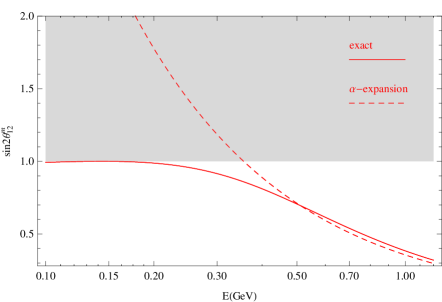
Note that the above $\alpha$-expansion of effective parameters requires not only $\alpha\ll 1$ but also $\alpha/A\ll 1$. If we look at the effective mixing angles in (21-24), we find that the $\alpha$-expansion of $\sin 2\theta_{12}^{m}$ may have a problem at $\alpha/A\sim 1$. In (22) we see $\sin 2\theta_{12}^{m}\sim\alpha/A$ which implies the correction from $\alpha$ is amplified by $1/A$, so the expansion may be not accurate if $A$ is small. We compare it with the exact value from Zaglauer and Schwarzer (1988) in figure 1, where the energy range is $0.1-1.2$GeV and matter density is 1.3$\textrm{g/}\textrm{cm}^{3}$ (the case of the T2K experiment). From figure 1 we see the expansion formula fits the exact solution well only at $E>0.5$ GeV but deviates from it quickly when $E<0.5$GeV. More seriously, when the energy goes below 0.35 GeV then $\sin 2\theta_{12}^{m}$ will be larger than $1$ (the gray region). This is because the unitarity of $\tilde{U}$ is badly violated.

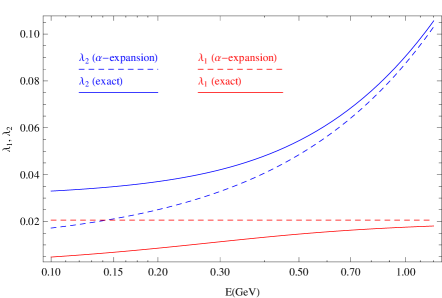
The other parameters suffering from the same problem are $\lambda_{1}$ and $\lambda_{2}$. We plot them with the exact solutions in figure 2. We see that below 0.3 GeV the effective mass square difference $\Delta\tilde{m}_{21}^{2}=m_{3}^{2}(\lambda_{2}-\lambda_{1})$ from the exact solution (solid curves) can be several times that of the $\alpha$-expansion (dashed curves), which also implies invalidity of the $\alpha$-expansion at low energies.

Figure 2: Compare the approximate formula of the eigenvalues $\lambda_{1}$ and $\lambda_{2}$ with the exact solution.

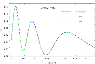
But interestingly, the formula of oscillation probability assembled from these inaccurate and even invalid pieces is very accurate, as shown in figure 3 where we use the same energy range and matter density as figure 1 and figure 2.

Figure 3: The plot shows that the conventional formula (blue solid curve) given by (1) is very accurate when used in T2K, in contrast with figure 1 and figure 2 where those effective parameters used to compute the probability are very inaccurate. All three order contributions ($\alpha^{0}$, $\alpha^{1}$ and $\alpha^{2}$) are also plotted (dashed curves) to show that all of them are indispensable to make (1) accurate in T2K.

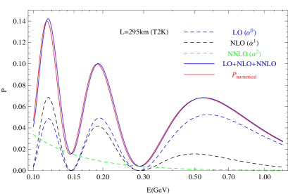
One argument might be that, the accuracy of $P$ is because $\sin 2\theta_{12}^{m}$ does not appear at the leading order (LO) of (1), but only at the next-to-leading order (NLO) and the next-to-next-to-leading order (NNLO) which are of order $\alpha^{1}$ and $\alpha^{2}$, respectively. This suppresses the effect of the inaccuracy from $\sin 2\theta_{12}^{m}$ shown in figure 1. But in figure 3 we see that at the second and third peaks (from right to left), the NLO and NNLO are comparable to the LO so the accuracy can not be explained by the NLO suppression.

It might be expected that the calculation at a higher order of $\alpha$ can explain this by finding some cancellations between errors. However, at a higher order, the accuracy in figures 1,2 turns out to be improved very little. Actually, as will be discussed in the next section, there is an underlying problem that some variables in the calculation are not differentiable at $\alpha=A=0$. For these variables, the expansion series including $\alpha/A$ can not even converge if $\alpha/A\gtrsim 1$. That is why a higher order calculation can not solve the accuracy problem.

3 Non-differentiabilities, singularities and branch cuts in the oscillating system

To reveal the key problem in the expansion, we start from an oversimplified but heuristic problem, series expansion of the following function

$$g(\alpha,A)=\sqrt{\alpha^{2}+A^{2}}.$$ (26)

If $\alpha$ is small, but $A$ is relatively not, then we can expand it in $\alpha$,

$$g(\alpha,A)=A+\frac{\alpha^{2}}{2A}+\alpha\mathcal{O}(\frac{\alpha^{3}}{A^{3}}).$$ (27)

Here we see $\alpha/A\ll 1$ is necessary to make eq.(27) accurate. If $A$ is much smaller than $\alpha$, then we can expand it in $A$ as $g(\alpha,A)=\alpha+A^{2}/(2\alpha)+\cdots$. But what if $A$ is close to $\alpha$? One may think that if A is close to $\alpha$, then both are small so we can make a double expansion of the function,

$$g(\alpha,A)=c_{0}+c_{1}\alpha+c_{2}A+\mathcal{O}(\alpha^{2},\alpha A,A^{2}),$$ (28)

where $c_{0}=g(0,0)$, $c_{1}$ and $c_{2}$ are the partial derivatives $\partial_{\alpha}g$ and $\partial_{A}g$ at $\alpha=A=0$. However, we cannot expand $\sqrt{\alpha^{2}+A^{2}}$ in this way because the partial derivatives $c_{1}$ and $c_{2}$ do not exist (as one can check explicitly). Geometrically this is easy to understand since $g=\sqrt{\alpha^{2}+A^{2}}$ is a cone in the $\alpha-A-g$ space. Expansion at the tip of the cone will certainly fail.

Actually the function (26) does exist in the eigenvalues of the oscillation system so in the original derivation of (1) $\alpha/A\ll 1$ has to be assumed. If we use formulae derived from such an expansion but simply ignore the condition $\alpha/A\ll 1$, then we are at the risk of getting total wrong results, such as $\sin 2\theta_{12}^{m}$>1 shown in Fig.1.

So basically the question is why for the oscillation probablity this problematic expansion works very well. This will be answered next by branch cut singularities.

First we look at the functions $\lambda_{k}(\alpha)$ which are defined by the exact solution of eigenvalues (14) and vary with $\alpha$, as shown in figure 4. Note that we consider $\lambda$’s as functions of $\alpha$ rather than $A$ (or $E$), since they are expanded with respect to $\alpha$.

Figure 4: The three eigenvalues given by eq.(14) as a function of $\alpha$. In the left plot, the matter effect parameter is $A=0.1$, corresponding to $E=1.2$GeV. In the right plot we take the limit $A\rightarrow 0$.

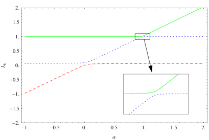
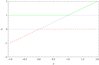
The left plot in figure 4 shows that the eigenvalues can be very close to another at level crossings (corresponding to resonances), but they never really go across another. They turn to different directions at level crossings which implies the behavior near the resonance is quite non-perturbative.

As we suppress $A$ close to zero, the curvatures at those turning points in figure 4 become larger and larger. Finally the curvatures go to infinite when $A\rightarrow 0$, which makes the curves turn suddenly at some points, then some singularities emerge. The right plot in figure 4 shows the $A\rightarrow 0$ limit. In this limit, the eigenvalues are continuous but not differentiable functions of $\alpha$.

Figure 5: Singularity in the eigenvalues and its origin from branch cut singularity. In the left plot the eigenvalues $\lambda_{1}$ and $\lambda_{2}$ from (14), as functions of $\alpha$ and $A$, have a singularity at (0,0). The singularity originates from the branch cut in (15). In the right plot we show the branch cut singularity of $\pm\sqrt{z}$ where $z=x+iy$.

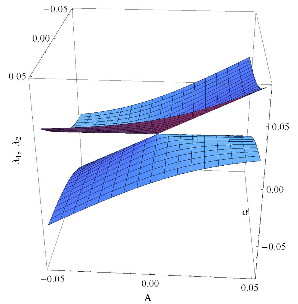
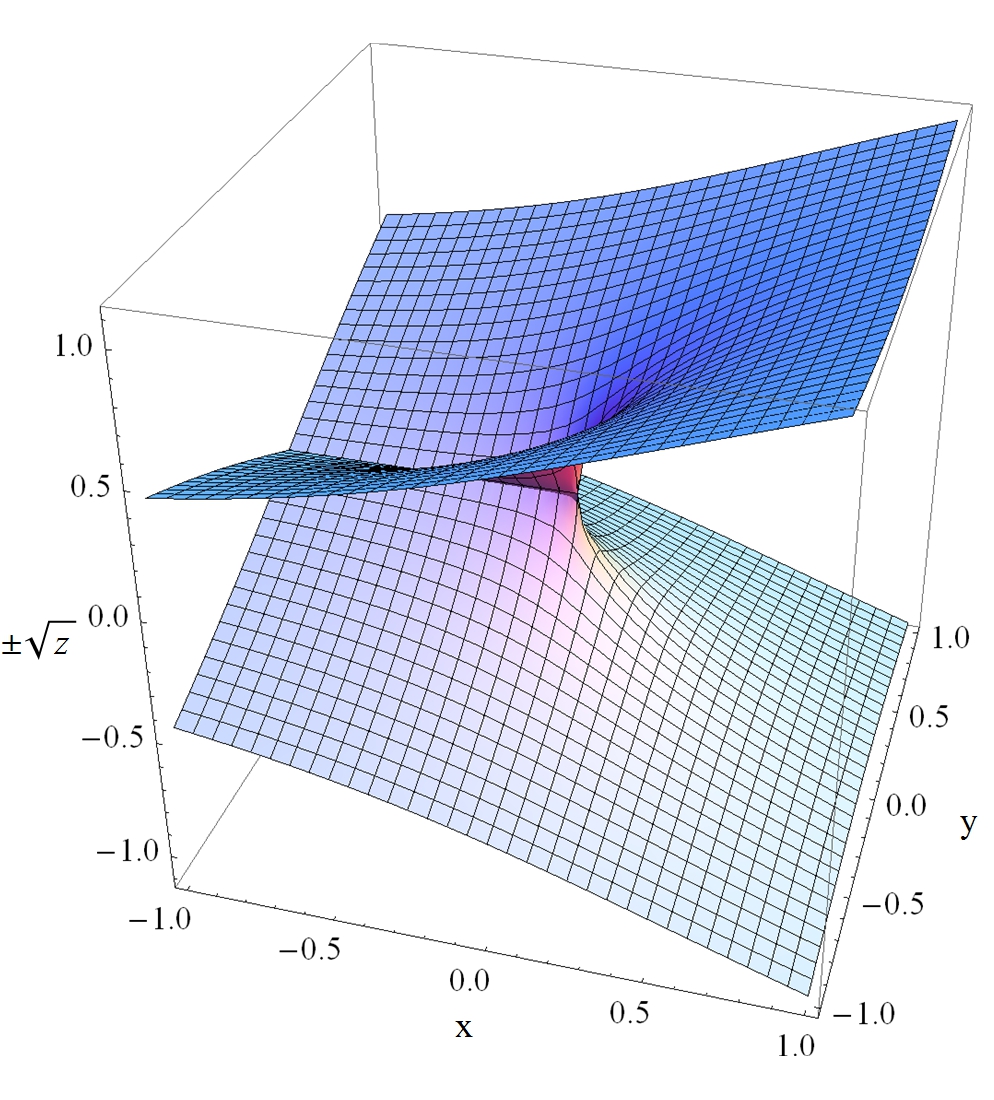
In the left plot of figure 5, we plot $\lambda_{1}$ and $\lambda_{2}$ as functions of $\alpha$ and $A$. It shows that there is a singularity (here we mean non-differentiable singularity) in the eigenvalues. The singularity is intrinsic and can not be removed by proper ordering of eigenvalues. So this implies that double expansion in $\alpha$ and $A$ does not work.

The intrinsic singularity in figure 5 is the kernel of the non-perturbativity problem in the oscillation system. It actually comes from a branch cut singularity. From eqs. (14) and (15) we see that $\lambda_{1,2,3}$ can be analytically expressed in terms of $b$, $c$ and $d$ and then further in terms of $\alpha$, $A$ and $u$ according to (13). They look like smooth analytic functions everywhere but they are actually not. Note that there is a square root and a cubic root in (15). Functions like $\sqrt{z}$ or $z^{1/3}$ have branch cut singularities which make them not analytic on the complex plane.

In the right plot in figure 5 we show the two branches of $\pm\sqrt{z}$ where $z\equiv x+iy$ connecting with each other at the branch cut (the line $y=0$ for $x<0$). At $x=0$ which is the end of the branch cut, there is a singularity. As one can check from (14) and (15), the branch cut singularity just corresponds to the singularity in the eigenvalues shown in the left plot.

4 Solution

Identifying that the singularity in the eigenvalues originates from the branch cut singularity makes a crucial step to solve the problem, since all branch cut singularities can be easily removed if the multi-branches collapse to one. For example, the branch cut singularity in $\sqrt{z}$ will disappear when it is squared, i.e. $(\sqrt{z})^{2}$ makes the two branches collapse and is singularity-free. Once the singularity is removed, $\alpha/A$ will not appear any more because $1/A$ will be absorbed by some continuous and smooth functions which we will see below. After the singularity problem is solved, we will mathematically show the conventional formula is accurate near the solar resonance.

The solution of the singularity problem can be summarized by the three key steps below:

1. Use the Cayley-Hamilton theoremMoler and Van Loan (1978); Ohlsson and Snellman (2000a, b) to express the $S$-matrix only in terms of the eigenvalues $\lambda_{1,2,3}$. The eigenvectors are not needed.

2. The singularity still exists in the eigenvalues but can be partially removed by the transformation

   $$\lambda_{\pm}=\frac{1}{2}(\lambda_{1}\pm\lambda_{2}),$$ (29)

   where it will be shown that $\lambda_{+}$ and $\lambda_{-}^{2}$ are singularity-free, though the singularity still exists in $\lambda_{-}$ since it is a branch cut singularity.

3. It turns out that $\lambda_{-}$ only appears in cosine function and the following function

   $$f(x)\equiv\frac{\sin x}{x},$$ (30)

   where $x$ is proportional to $\lambda_{-}$. Note that $f(x)$ is smooth everywhere, even at $x=0$. Since $f(x)=1-\frac{x^{2}}{6}+\frac{x^{4}}{120}+...$ and $\cos x=1-\frac{x^{2}}{2}+\frac{x^{4}}{24}+...$ are actually functions of $x^{2}\propto\lambda_{-}^{2}$ which is singularity-free, the singularity is removed.

In short, we will first make the $S$-matrix only depend on $(\lambda_{1},\lambda_{2},\lambda_{3})$ and then after the transformation from $(\lambda_{1},\lambda_{2},\lambda_{3})$ to $(\lambda_{-}^{2},\lambda_{+},\lambda_{3})$, the singularity in the $S$-matrix will be explicitly removed. Next we will show the calculation in detail.

The Cayley-Hamilton theorem is a theorem in linear algebra which states that if $p(\lambda)$ is the characteristic polynomial of a matrix $A$ [for example the left-handed side of eq.(12)], then substituting the matrix $A$ for $\lambda$ in this polynomial results in the zero matrix, i.e. $p(A)=0.$ Take the example of eq.(12), this means $M^{3}+bM^{2}+cM+d=0$ or

$$M^{3}=-(bM^{2}+cM+d).$$ (31)

This implies $e^{M}=I+M+M^{2}/2!+...$ can be expressed by a polynomial of $M$ with finite terms since all $M^{n}$ with $n\geq 3$ can be converted to linear combinations of $I,M,M^{2}$ by eq.(31). So we have

$$e^{-itM}=s_{0}I+s_{1}M+s_{2}M^{2},$$ (32)

where we put a $-it$ to be used later. The coefficient $s_{0}$, $s_{1}$ and $s_{2}$ can be determined in various methodsMoler and Van Loan (1978) such as the Lagrange interpolation or the Newton interpolation. They have been computed in Ohlsson and Snellman (2000a, b),

$$s_{0} = \frac{-1}{\Delta_{\lambda}}[e^{-it\lambda_{3}}\lambda_{1}\lambda_{2}(\lambda_{1}-\lambda_{2})+e^{-it\lambda_{1}}\lambda_{2}\lambda_{3}(\lambda_{2}-\lambda_{3})+e^{-it\lambda_{2}}\lambda_{1}\lambda_{3}(\lambda_{3}-\lambda_{1})],$$ (33)

$$s_{1} = \frac{1}{\Delta_{\lambda}}[e^{-it\lambda_{3}}(\lambda_{1}^{2}-\lambda_{2}^{2})+e^{-it\lambda_{1}}(\lambda_{2}^{2}-\lambda_{3}^{2})+e^{-it\lambda_{2}}(\lambda_{3}^{2}-\lambda_{1}^{2})],$$ (34)

$$s_{2} = \frac{-1}{\Delta_{\lambda}}[e^{-it\lambda_{3}}(\lambda_{1}-\lambda_{2})+e^{-it\lambda_{1}}(\lambda_{2}-\lambda_{3})+e^{-it\lambda_{2}}(\lambda_{3}-\lambda_{1})],$$ (35)

where

$$\Delta_{\lambda}\equiv(\lambda_{1}-\lambda_{2})(\lambda_{2}-\lambda_{3})(\lambda_{3}-\lambda_{1}).$$ (36)

From eq.(5) and (9), the $S$-matrix is

$$S=e^{-iHL}=e^{-i\frac{m_{1}^{2}L}{2E}}e^{-2i\Delta M},$$ (37)

where

$$M=U\left(\begin{array}[]{ccc}0\\ &\alpha\\ &&1\end{array}\right)U^{\dagger}+\left(\begin{array}[]{ccc}A\\ &0\\ &&0\end{array}\right).$$ (38)

So we can identify $t=2\Delta$ to use eq.(32) directly.

Now the transition amplitude of $\nu_{\mu}\rightarrow\nu_{e}$ is $S_{e\mu}=s_{0}I_{12}+s_{1}M_{12}+s_{2}(M^{2})_{12}$ but because $I$ is an identity matrix, $S_{e\mu}$ can be written as two terms

$$S_{e\mu}=s_{1}M_{12}+s_{2}(M^{2})_{12},$$ (39)

which implies we do not need to compute $s_{0}$ for the appearance probability.

The denominator $\Delta_{\lambda}$ in $s_{1}$ and $s_{2}$ is possible to be zero, but we will show next that $s_{1}$ and $s_{2}$ are not divergent at $\Delta_{\lambda}=0$ and smooth (differentiable) everywhere. For example the singularity from $\lambda_{1}-\lambda_{2}=0$ can be removed by the transformation $\lambda_{\pm}=\frac{1}{2}(\lambda_{1}\pm\lambda_{2})$. This singularity is the only one that confronts us in the energy range of current experiments.

According to Vieta’s formulas for a cubic equation,

$$\lambda_{1}+\lambda_{2}+\lambda_{3}=-b,\thinspace\lambda_{1}\lambda_{2}\lambda_{3}=-d,$$ (40)

we have $\lambda_{1}+\lambda_{2}=-b-\lambda_{3}$ and $\lambda_{1}\lambda_{2}=-d\lambda_{3}^{-1}$. Therefore

$$\lambda_{+}=\frac{1}{2}(-b-\lambda_{3}),\thinspace\lambda_{-}^{2}=\lambda_{+}^{2}+d\lambda_{3}^{-1},$$ (41)

where $b$, $d$ are apparently free from the singularity [as shown in eq.(13)] and $\lambda_{3}$ is also singularity-free (shown in figure 4, see also the proof in the Appendix). So $\lambda_{+}$ and $\lambda_{-}^{2}$ are singularity-free. Note that, however, $\lambda_{-}$ has a singularity originating from the branch cut singularity, which can be seen from figure 5.

After the transformation $\lambda_{\pm}=\frac{1}{2}(\lambda_{1}\pm\lambda_{2})$, $s_{1}$ and $s_{2}$ are given by

$$s_{1}=\frac{-2\lambda_{+}e^{-it\lambda_{3}}+e^{-it\lambda_{+}}[2\lambda_{+}\cos(\lambda_{-}t)+it(\lambda_{+}^{2}+\lambda_{-}^{2}-\lambda_{3}^{2})f(\lambda_{-}t)]}{\lambda_{3}^{2}-2\lambda_{+}\lambda_{3}-d\lambda_{3}^{-1}},$$ (42)

$$s_{2}=\frac{e^{-it\lambda_{3}}+e^{-it\lambda_{+}}[-\cos(\lambda_{-}t)+it(\lambda_{3}-\lambda_{+})f(\lambda_{-}t)]}{\lambda_{3}^{2}-2\lambda_{+}\lambda_{3}-d\lambda_{3}^{-1}}.$$ (43)

We see they depend only on $\lambda_{3},$ $\lambda_{+}$ , $\lambda_{-}$ and $d$ which are all continuous and smooth functions except for $\lambda_{-}$. But since $\lambda_{-}$ only appears in $\cos(\lambda_{-}t)$ and $f(\lambda_{-}t)$ which are actually functions of $\lambda_{-}^{2}$ ( note that $\cos(x)=1-\frac{x^{2}}{2}+\frac{x^{4}}{24}+...$ and $f(x)=1-\frac{x^{2}}{6}+\frac{x^{4}}{120}+...$), we come to the conclusion that $s_{1}$ and $s_{2}$ are continuous and smooth functions of $\alpha$ and $A$.

Now that we have expressed the $S$-matrix in terms of $(\lambda_{3},\lambda_{+},\lambda_{-}^{2})$ and thus removed the singularity, expansion in $\alpha$ will not suffer from any problems. The $\alpha/A$ appears in section 2 will not appear any more if we use eqs.(42-43) to compute the probability.

Define

$$p=U_{e3}U_{\mu 3}^{*},\thinspace q=U_{e2}U_{\mu 2}^{*},$$ (44)

we have

$$S_{e\mu}=p[s_{1}+s_{2}(1+A)]+q\alpha[s_{1}+s_{2}(\alpha+A)].$$ (45)

We call the two terms in eq.(45) as $p$ term and $q$ term respectively. From eqs.(42-43) we have

$$p\textrm{ term} = \frac{p}{\lambda_{3}^{2}-2\lambda_{+}\lambda_{3}-d\lambda_{3}^{-1}}\left[e^{-it\lambda_{3}}(\lambda_{3}-\alpha)-e^{-it\lambda_{+}}\cos(\lambda_{-}t)(\lambda_{3}-\alpha)\right.$$ (46)

$$\left.+ite^{-it\lambda_{+}}f(\lambda_{-}t)(\lambda_{+}\lambda_{3}+\alpha\lambda_{+}-d-\alpha\lambda_{3})\right],$$

$$q\textrm{ term} = \frac{q\alpha}{\lambda_{3}^{2}-2\lambda_{+}\lambda_{3}-d\lambda_{3}^{-1}}\left[e^{-it\lambda_{3}}(\lambda_{3}-1)-e^{-it\lambda_{+}}\cos(\lambda_{-}t)(\lambda_{3}-1)\right.$$ (47)

$$\left.-ite^{-it\lambda_{+}}f(\lambda_{-}t)(\lambda_{3}^{2}-2\lambda_{+}\lambda_{3}-d\lambda_{3}^{-1}+(\lambda_{3}-1)(\lambda_{3}-\lambda_{+}))\right].$$

So far we have not taken any approximation. Then we will use the approximation

$$\lambda_{3}=1+\mathcal{O}(s_{13}^{2}A),$$ (48)

which is derived in the Appendix. With this approximation, from eq.(41) we have

$$2\lambda_{+}=A+\alpha+\mathcal{O}(s_{13}^{2}A),\thinspace\lambda_{-}^{2}=\lambda_{+}^{2}-\frac{A\alpha c_{12}^{2}c_{13}^{2}}{1+\mathcal{O}(s_{13}^{2}A)}.$$ (49)

Since the $p$ term and $q$ term have been expressed in terms of singularity-free quantities $\lambda_{3}$, $\lambda_{+}$ and $\lambda_{-}^{2}$, we can use (48,49) to compute them. The calculation is straightforward (see the Appendix) and the result is

$$p\textrm{ term}=p\frac{e^{-2i\Delta}-e^{-2iA\Delta}}{1-A}+\mathcal{O}(\Delta s_{13}^{3}A)+\mathcal{O}(\Delta^{2}s_{13}\alpha A),$$ (50)

$$q\textrm{ term}=-2iq\alpha e^{-i(A+\alpha)\Delta}\frac{\sin(\bar{A}\Delta)}{\bar{A}}+\mathcal{O}(\Delta\alpha s_{13}^{2}A),$$ (51)

where

$$\bar{A}\equiv\sqrt{(A+\alpha)^{2}-4A\alpha c_{12}^{2}c_{13}^{2}}.$$ (52)

The oscillation probability is

$$|p\textrm{ term}+q\textrm{ term}|^{2}$$ (53)

$$= |p\frac{e^{-2i\Delta}-e^{-2iA\Delta}}{1-A}-2iq\alpha e^{-i(A+\alpha)\Delta}\frac{\sin(\bar{A}\Delta)}{\bar{A}}+\mathcal{O}(\Delta s_{13}^{3}A)+\mathcal{O}(\Delta^{2}s_{13}\alpha A)|^{2}$$

$$= P^{(A)}+\mathcal{O}(s_{13}^{4}A\Delta)+\mathcal{O}(s_{13}^{2}\alpha A\Delta^{2}),$$

where $P^{(A)}$ is defined as

$$P^{(A)}=|p\frac{e^{-2i\Delta}-e^{-2iA\Delta}}{1-A}-2iq\alpha e^{-i(A+\alpha)\Delta}\frac{\sin(\bar{A}\Delta)}{\bar{A}}|^{2}.$$ (54)

To derive (1), we need to expand the modulus squared of (54),

$$P^{(A)}=|p\textrm{ term}|^{2}+2\textrm{Re}[\overline{p\textrm{ term}}\times q\textrm{ term}]+|q\textrm{ term}|^{2},$$ (55)

where $|p\textrm{ term}|^{2}$, $|q\textrm{ term}|^{2}$ and the cross term are computed in the appendix and the result is

$$|p\textrm{ term}|^{2}=4s_{13}^{2}c_{13}^{2}s_{23}^{2}\frac{\sin^{2}(1-A)\Delta}{(1-A)^{2}},$$ (56)

$$|q\textrm{ term}|^{2}=4\alpha^{2}s_{12}^{2}c_{12}^{2}c_{23}^{2}\frac{\sin^{2}(A\Delta)}{A^{2}}+\mathcal{O}(\alpha^{4}\Delta^{4})+\mathcal{O}(A\alpha^{3}\Delta^{4})+\mathcal{O}(\alpha^{2}s_{13}\Delta^{2})),$$ (57)

$$2\textrm{Re}[\overline{p\textrm{ term}}\times q\textrm{ term}]=8\alpha\frac{J_{CP}}{s_{\delta}}\cos(\Delta+\delta)\frac{\sin A\Delta}{A}\frac{\sin(1-A)\Delta}{1-A}+\mathcal{O}(\alpha s_{13}^{2}\Delta)+\mathcal{O}(s_{13}\alpha^{2}\Delta).$$ (58)

Now the conventional formula (1) can be analytically justified near and below the solar resonance. Here we denote it as $P^{(B)}$ . We can see that the first and last terms of $P^{B}$ just correspond to eqs.(56,57) respectively and the middle term in $P^{(B)}$ corresponds to the cross term (58). Combine the analytic errors, we have

$$P^{(B)}-P^{(A)}=\mathcal{O}(s_{13}^{2}\alpha\Delta)+\mathcal{O}(s_{13}\alpha^{2}\Delta^{2})+\mathcal{O}(\alpha^{3}A\Delta^{4})+\mathcal{O}(\alpha^{4}\Delta^{4}),$$ (59)

which implies that the conventional formula is accurate up to the $\mathcal{O}$-terms above and the $\mathcal{O}$-terms in (53). We see there is no $\alpha/A$ in all these $\mathcal{O}$’s, so we draw the conclusion that the bound (3) which originally requires $\alpha/A\ll 1$ can be safely removed. The conventional formula is still accurate without this bound, as long as these $\mathcal{O}$-terms are small.

According to eq.(53), the error of $P^{(A)}$ is $\delta P^{(A)}=\mathcal{O}(s_{13}^{4}A\Delta)+\mathcal{O}(s_{13}^{2}\alpha A\Delta^{2})$. Taking T2K as an example, for $E=0.25$GeV which is below the conventional domain of validity, we have $A\simeq 0.02$ and $\Delta\simeq 3.7$. This gives $s_{13}^{2}\alpha A\Delta^{2}\simeq 2\times 10^{-4}$ and $s_{13}^{4}A\Delta\simeq 4\times 10^{-5}$. The error is very small and the dominant correction would be $\mathcal{O}(s_{13}^{2}\alpha A\Delta^{2})$ if we want to improve the accuracy. Actually, if we only concern ourselves with the $\Delta\gtrsim 1$ region, then $\mathcal{O}(s_{13}^{2}\alpha A\Delta^{2})$ is larger than $\mathcal{O}(s_{13}^{4}A\Delta)$ since $s_{13}^{2}\alpha\simeq s_{13}^{4}$. Therefore we expect that typically $\mathcal{O}(s_{13}^{2}\alpha A\Delta^{2})$ is the principal source of the error of $P^{(A)}$. For the same set of parameter values, the four terms in eq.(59) have the values, $s_{13}^{2}\alpha\Delta\simeq 3\times 10^{-3}$, $s_{13}\alpha^{2}\Delta^{2}\simeq 2\times 10^{-3}$ and $\alpha^{3}A\Delta^{4}\simeq\alpha^{4}\Delta^{4}\simeq 1\times 10^{-4}$. So the dominant errors of $P^{(B)}$ are $\mathcal{O}(s_{13}^{2}\alpha\Delta)$ and $\mathcal{O}(s_{13}\alpha^{2}\Delta^{2})$. Note that they do not depend on $A$, which implies that the main source of inaccuracy of $P^{(B)}$ is not due to inadequately accounting for the matter effect contribution, but rather than due to an insufficient expansion of the small phase $\alpha\Delta$. Though the phase $\alpha\Delta$ is small, terms quadratic in $\alpha\Delta$ would not be negligible if we want to improve its accuracy. In conclusion, the dominant errors of $P^{(A)}$ and $P^{(B)}$ are given by $\mathcal{O}(s_{13}^{2}\alpha A\Delta^{2})$ and $\mathcal{O}(s_{13}^{2}\alpha\Delta)+\mathcal{O}(s_{13}\alpha^{2}\Delta^{2})$, respectively.

5 Numerical verification

As our study of the problem is originally motivated by the fact that T2K covers the solar resonance, we would like to numerically verify our analysis in that case first. The matter density in T2K is $\rho=2.6\textrm{g}/\textrm{cm}^{3}$Abe et al. (2013b) so we take the electron density to be $N_{e}=1.3N_{A}/\textrm{cm}^{3}$ under the assumption that for matter $Z/A=1/2$ in average.

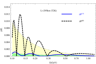
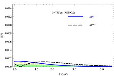
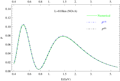
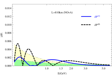
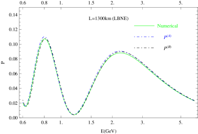
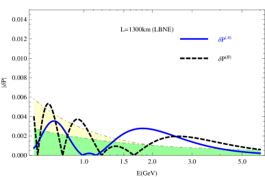
Figure 6 shows that both $P^{(A)}$ and $P^{(B)}$ are accurate enough for practical use while the new formula $P^{(A)}$ has better accuracy than the conventional formula $P^{(B)}$. We also plot the analytic errors according to (53) and (59) in the right panel of figure 6, using light green and yellow shades. The actual residuals defined as $|\delta P|=|P-P_{\textrm{numerical}}|$ where $P_{\textrm{numerical}}$ is the numerical solution are well compatible with analytic estimation, which implies the errors are correctly estimated. Therefore figure 6 verifies both $P^{(A,B)}$ and $\delta P^{(A,B)}$ in the T2K case.

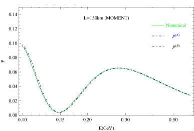
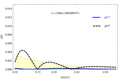
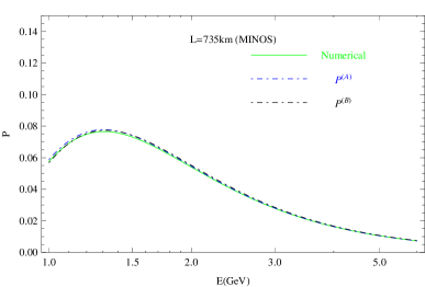
Besides T2K, we also show the accuracies of these formulae in other accelerator neutrino experiments. The information of the baselines and neutrino energies are listed in table 1 and for simplicity we take the same matter density as T2K for all the other experiments, since the neutrino beams in these experiments only go though the earth crust. We see again that in current or future accelerator neutrino experiments, the formulae are accurate enough for practical use and the errors are well described by our analytic estimation.

Figure 6: A comparison of the approximate oscillation formulae with the numerical solution to (5) in the T2K case. The left plot shows that all these approximate formulae are very accurate and the errors are negligible for practical use. The right plot shows that the residuals defined as $|\delta P|=|P-P_{\textrm{numerical}}|$ are consistent with our analytic estimation of the error, which are represented by green and yellow shades for $\delta P^{(A)}$ and $\delta P^{(B)}$ respectively.

Experiments	$L$/km	$E$/GeV	$A(E/\textrm{GeV})$	Refs
MOMENT	150	$\sim 0.3$	$0.024$	Cao et al. (2014)
T2K	295	$0.6\thinspace(0.1\rightarrow 1.2)$	$0.048\thinspace(0.008\rightarrow 0.096)$	Abe et al. (2013a, 2014)
MINOS	735	$3\thinspace(1\rightarrow 6)$	$0.24\thinspace(0.08\rightarrow 0.48)$	Adamson et al. (2011)
NOvA	810	$\sim 2$	$0.16$	Ayres et al. (2004); Patterson (2013)
LBNE	1300	$\sim 2.5$	$0.20$	Adams et al. (2013)

Table 1: Baseline lengths and neutrino energies of current and future accelerator neutrino experiments. For T2K and MINOS there are both peaks and ranges (in parentheses) of neutrino energies according to the references while for the other experiments we only show the general energies. The electron density is $N_{e}=1.3N_{A}/\textrm{cm}^{3}$ in our calculation, so we also show the values of $A$ corresponding to the energies.

Figure 7: Similar plots to figure 6 but for some other accelerator neutrino experiments. For more details, see the T2K case in figure 6.

Although computers are becoming more powerful, it is still desirable to have efficient methods of computation. For example, the $\chi^{2}$-fit in a high dimensional parameter space (including both oscillation parameters and experiment parameters) is always extremely time-consuming. When nuisance parameters are being marginalized, the likelihood function has to be invoked an enormous amount of times to complete a sub-process of minimization (only for the frequentist treatment, the Bayesian approach usually needs much more computations). The package GLoBES Huber et al. (2005, 2007) which was designed for simulation of neutrino oscillation experiments has optimized the diagonalization procedure Kopp (2008) combining the QL decomposition with additional developed algorithms. This is not necessary for oscillations in constant density matter, where a simple analytical formula performs better (GLoBES allows users to replace the probability engine with a user-defined function). In this case, we recommend the use of $P^{(A)}$ instead. A simple test on Mathematica 8.0 with Intel Core i7 CPU shows that $10^{5}$ evaluations of $P^{(A)}$ and $P^{(B)}$ cost $4.7$ and $5.6$ seconds, which implies $P^{(A)}$ can be computed at a speed not slower than $P^{(B)}$.

Finally there is one issue related to the solar resonance to be discussed. Strictly speaking, the matter effect can be safely regarded as a small perturbative effect only if $2\sqrt{2}G_{F}N_{e}E$ is much less than $\Delta m_{21}^{2}$ ($A\ll\alpha$), i.e. only the region between the vacuum limit and the solar resonance can be regarded as the truly small-$A$ region, where no physics can be changed greatly by the matter effect. Typically LBL accelerator neutrino experiments are in the region between the solar resonance and the atmospheric resonance which we can refer to as medium-$A$ region. Note that originally $A$ can not be treated perturbatively in the medium-$A$ regionFreund (2001). From the small-$A$ region to the medium-$A$ region, the solar mixing will experience a resonance. It is interesting that, according to the formulae we derived , the contribution from the matter effect passes through the resonance gradually without showing any resonances, despite the solar mixing being affected drastically in that region (note that the solar mixing has sizable contributions to these experiments). In other words, the region with a perturbative matter correction can be extended from the small-$A$ region to the medium-$A$ region for current LBL accelerator neutrino experiments.

6 Conclusion

The conventional formula obtained by an expansion in the mass hierarchy parameter $\alpha=\Delta m_{21}^{2}/\Delta m_{31}^{2}\approx 0.03$ turns out to be very accurate near the solar resonance, as shown in figure 3 though the effective masses and effective mixing angles computed in the $\alpha$-expansion are inaccurate or even invalid at this region, as shown in figure 1 and figure 2. So it is interesting that the intermediate inaccuracies cancel each other out in the final result.

We have shown that the inaccuracies are because the expansion is too close to the branch cut singularity in the eigenvalues. This singularity is inherent in the eigenvalues so it cannot be removed by interchanging eigenvalues. But certain combinations of them such as their sum of the eigenvalues $\lambda_{1}+\lambda_{2}$ do not have the singularity, and the oscillation probability only depends on these singularity-free combinations. By computing the probability in this way, we have analytically proven that the conventional formula is still accurate near the solar resonance.

A new oscillation formula $P^{(A)}$ in (54) which might be practically useful is derived when we try to prove the accuracy of the conventional one. Both the conventional and the new formulae are very accurate in various accelerator neutrino experiments for baseline lengths varying from $150$km (MOMENT) to $1300$km (LBNE), as shown in figures 6 and 7. We have also estimated the analytic errors for these formulae.

Appendix A Some details of analytic calculations

A.1 Simplify the $p$ term and $q$ term

Here we show how to simplify the $p$ term and $q$ term step by step. All the approximations in the calculation should be analytically treated so we use $\mathcal{O}()$ instead of $\approx$.

The first result we will derive is eq.(48). Note that the cubic equation (12) has the following identity

$$b+c+d=As_{13}^{2}(\alpha-1)-1,$$ (60)

which provides a fast way to compute $\lambda_{3}$ as follow. We assume $\lambda_{3}=1+x$ with $x\ll 1$ and replace the $\lambda$ in the cubic equation (12) with $1+x$. Then the leading order vanishes and the next-to-leading order(NLO) gives

$$3x+x(2b+c)+\mathcal{O}(x^{2})=As_{13}^{2}(1-\alpha),$$ (61)

which implies $x=\mathcal{O}(s_{13}^{2}A)$ while the explicit form of $x$ is not important here.

Therefore from eq.(41) we have

$$2\lambda_{+}=A+\alpha+x,\thinspace\lambda_{-}^{2}=\lambda_{+}^{2}-\lambda_{1}\lambda_{2},\thinspace\lambda_{1}\lambda_{2}=\frac{A\alpha u_{1}^{2}}{1+x},$$ (62)

so the $q$ term can be greatly simplified,

$$q\textrm{ term} = \frac{q\alpha[\mathcal{O}(\Delta x)+ite^{-it\lambda_{+}}f(\lambda_{-}t)(\lambda_{3}^{2}-2\lambda_{+}\lambda_{3}-d\lambda_{3}^{-1}+x(\lambda_{3}-\lambda_{+}))]}{\lambda_{3}^{2}-2\lambda_{+}\lambda_{3}-d\lambda_{3}^{-1}}$$ (63)

$$= -itq\alpha e^{-it\lambda_{+}}f(\lambda_{-}t)+\mathcal{O}(\alpha\Delta x)$$

$$= -2iq\alpha e^{-i(A+\alpha+x)\Delta}\sin(\bar{A}\Delta)/\bar{A}+\mathcal{O}(\alpha\Delta s_{13}^{2}A),$$

where $\bar{A}\equiv\sqrt{(A+\alpha)^{2}-4A\alpha c_{12}^{2}c_{13}^{2}}$ or $\bar{A}^{2}=4\lambda_{-}^{2}$.

$$p\textrm{ term} = \frac{p}{(1-A)(1-\alpha)+\mathcal{O}(x)+\mathcal{O}(\alpha A)}\left[e^{-it}(1-\alpha)-e^{-it\lambda_{+}}\cos(\lambda_{-}t)(1-\alpha)+\mathcal{O}(x)\right.$$ (64)

$$\left.+ite^{-it\lambda_{+}}f(\lambda_{-}t)\left((1-\alpha)(A-\alpha)/2+\mathcal{O}(\alpha A)+\mathcal{O}(\alpha x)+\mathcal{O}(\lambda_{+}x)\right)\right]$$

$$= \frac{p\left[e^{-it}(1-\alpha)-e^{-it\lambda_{+}}\cos(\lambda_{-}t)(1-\alpha)+ite^{-it\lambda_{+}}f(\lambda_{-}t)(1-\alpha)(A-\alpha)/2\right]}{(1-A)(1-\alpha)}$$

$$+p\left[\mathcal{O}(\Delta x)+\mathcal{O}(\Delta\alpha A)\right]$$

$$= \frac{p}{1-A}\left[e^{-it}-e^{-it\lambda_{+}}\cos(\lambda_{-}t)+ite^{-it\lambda_{+}}f(\lambda_{-}t)\frac{A-\alpha}{2}\right]$$

$$+p\left[\mathcal{O}(\Delta x)+\mathcal{O}(\Delta\alpha A)\right].$$

Since $\cos(\lambda_{-}t)$ and $f(\lambda_{-}t)$ only depend on $\lambda_{-}^{2}=(\alpha-A)^{2}/4-\alpha A(1-u_{1}^{2})$ we have

$$\cos(\lambda_{-}t)-itf(\lambda_{-}t)\frac{A-\alpha}{2}=\cos(\frac{\alpha-A}{2}t)-itf(\frac{\alpha-A}{2}t)\frac{A-\alpha}{2}+\mathcal{O}(\alpha A\Delta^{2}).$$

So finally we get

$$p\textrm{ term}=\frac{p}{1-A}\left[e^{-it}-e^{-itA}\right]+\mathcal{O}(s_{13}^{3}A\Delta)+\mathcal{O}(s_{13}\alpha A\Delta^{2}).$$ (65)

A.2 Calculate $P^{(B)}-P^{(A)}$

After expanding the square in $P^{(A)}$, we see the square term of $p$ equals to the leading term in $P^{(B)}$. As for the square term of $q$, since we have

$$q=s_{12}c_{13}c_{12}c_{23}+\mathcal{O}(s_{13}),$$ (66)

so the differences of the corresponding term in $P^{(B)}$ and the $q$ square term is

$$4\alpha^{2}s_{12}^{2}c_{12}^{2}c_{23}^{2}\frac{\sin^{2}(A\Delta)}{A^{2}}-(q\textrm{ square term})$$ (67)

$$= 4\alpha^{2}\left[s_{12}^{2}c_{12}^{2}c_{23}^{2}(\frac{\sin^{2}(A\Delta)}{A^{2}}-\frac{\sin^{2}(\bar{A}\Delta)}{\bar{A}^{2}})+\mathcal{O}(s_{13}\Delta^{2})\right]$$

$$= 4\alpha^{2}\left[2\Delta^{2}\frac{1}{6}(\bar{A}^{2}-A^{2})+\mathcal{O}(s_{13}\Delta^{2})\right]$$

$$= \mathcal{O}(\alpha^{4}\Delta^{4})+\mathcal{O}(A\alpha^{3}\Delta^{4})+\mathcal{O}(\alpha^{2}s_{13}\Delta^{2})),$$

where we have used the following approximation for $f(x)\equiv\frac{1}{x}\sin x$

$$f(\bar{A}\Delta)-f(A\Delta)=-\frac{1}{6}(\bar{A}^{2}\Delta^{2}-A^{2}\Delta^{2})+\mathcal{O}(A^{4}\Delta^{4},\bar{A}^{4}\Delta^{4}).$$

The remaining term is the cross term, computed as follows

$$2\textrm{Re}[\overline{p\textrm{ term}}\times q\textrm{ term}]$$

$$= 2\textrm{Re}[-2i\alpha\bar{p}q\frac{e^{2i\Delta}-e^{2iA\Delta}}{1-A}e^{-i(A+\alpha)\Delta}\frac{\sin(\bar{A}\Delta)}{\bar{A}}]$$

$$= 2\textrm{Re}[4\alpha(\frac{J_{CP}}{s_{\delta}}+\mathcal{O}(s_{13}^{2}))e^{i(\Delta-\alpha\Delta+\delta)}\frac{\sin[(1-A)\Delta]}{1-A}\frac{\sin(\bar{A}\Delta)}{\bar{A}}]$$

$$= 8\alpha[\frac{J_{CP}}{s_{\delta}}+\mathcal{O}(s_{13}^{2})][\cos(\Delta+\delta)+\mathcal{O}(\Delta\alpha)]\frac{\sin[(1-A)\Delta]}{1-A}[\frac{\sin(A\Delta)}{A}+\mathcal{O}(\alpha A\Delta^{3})+\mathcal{O}(\Delta^{3}\alpha^{2})]$$

$$= 8\alpha\frac{J_{CP}}{s_{\delta}}\cos(\Delta+\delta)\frac{\sin(A\Delta)}{A}\frac{\sin[(1-A)\Delta]}{1-A}$$ (70)

$$+\mathcal{O}(\alpha s_{13}^{2}\Delta)+\mathcal{O}(s_{13}\alpha^{2}\Delta)+\frac{1}{6}s_{13}\mathcal{O}(\alpha^{3}\Delta^{3},\alpha^{2}A\Delta^{3}),$$

where $p=s_{13}c_{13}s_{23}e^{-i\delta}$ has been used. Combine the result from eqs.(67) and (70), we have

$$P^{(B)}-P^{(A)}=\mathcal{O}(s_{13}^{2}\alpha\Delta)+\mathcal{O}(s_{13}\alpha^{2}\Delta^{2})+\mathcal{O}(\alpha^{3}A\Delta^{4})+\mathcal{O}(\alpha^{4}\Delta^{4}).$$ (71)