On the asymmetry of electroproduction of pions in double longitudinally polarized process
Abstract
We study the azimuthal asymmetry in double polarized semi-inclusive pion production by considering dynamical twist-3 effects. In particular, we evaluate the role of the transverse momentum dependent distributions and on the asymmetry. Using two different sets of spectator model results for these distributions, we predict the asymmetry of , , and at the kinematic configuration available at CLAS, HERMES and COMPASS. Our estimates show that the asymmetries are positive for all the pions and could be accessed by CLAS and HERMES. We also find that gives the dominant contribution to the asymmetry, while the contribution of is almost negligible.
pacs:
12.39.-x, 13.60.-r, 13.88.+eI Introduction
Nowadays it is very clear that a better understanding on the nucleon structure can be achieved if one goes beyond the collinear picture to take into account the transverse degree of freedom of partons. Early investigation Cahn on the unpolarized semi-inclusive deep inelastic scattering (SIDIS) demonstrated that the intrinsic transverse motion of quarks can give rise to a asymmetric distribution of the final state hadron. This mechanism, usually called as the Cahn effect, provides a useful tool to probe the partonic transverse momentum which is still less understood so far, although the effect appears kinematically at the subleading order of inverse hard scale. The same idea was then explored further by several experimental and theoretical studies Ashman:1991cj ; Aubert:1983cz ; Arneodo:zpc34 ; Adams:1993hs ; Mkrtchyan:2007sr ; Osipenko:2008aa ; Airapetian:2012yg ; Adolph:2014npb ; Anselmino:2005prd ; Schweitzer:2010tt ; Boglione:2011 to give constraints on the transverse structure of nucleon, i.e., the effect was applied Anselmino:2005prd ; Schweitzer:2010tt to extract the average values of the intrinsic transverse momenta of quarks inside the nucleon from SIDIS Ashman:1991cj ; Aubert:1983cz ; Arneodo:zpc34 ; Adams:1993hs or Drell-Yan data Conway:1989fs .
Recently, in a new study Anselmino:2006yc the Cahn effect was extended to the case of double longitudinally polarized SIDIS, prediciting a similar azmithual asymmetry that originates from the transverse momentum dependent (TMD) helicity distribution function . Due to the positive value of and quark dominance, the asymmetry based on the Cahn effect was found to be negative for both the charged and neutral pions in the case of proton target.
In this work, we will study the azimuthal asymmetry in double longitudinally polarized SIDIS in an alternative approach, that is, to employ dynamical twist-3 effects. As shown in Ref. Bacchetta:0611265 , the polarized structure function that associated with the asymmetry can be expressed in terms of the twist-3 TMD distribution/fragmentation function combined with the twist-2 fragmentation/distribution function. Particularly, two twist-3 TMD distributions appear in the convolutions: the T-even distribution and the T-odd distribution . The former one can be decomposed into the following form via the equation of motion relation Mulders:1995dh
| (1) |
Taking the component from in the above equation is equivalent to adopting the Cahn effect. In this study we will consider the effect of the entire twist-3 distribution . In addition, we also take into account the contribution of coupled with the Collins fragmentation function Collins:1993npb . We calculate these two TMD distributions of valence quarks inside the proton by employing the spectator diquark model and predict the corresponding asymmetry for charged and neutral pions at the kinematics of JLab, HERMES and COMPASS. We note that sizable dynamical twist-3 effects may also appear in other processes which involve different polarizations of the lepton beam and the nucleon target Airapetian:2005jc ; hermes07 ; Alekseev:2010dm ; Aghasyan:2011ha ; Gohn:2014zbz ; Parsamyan:2014uda ; Metz:2004je ; Bacchetta:2004zf ; Mao:2012dk ; Song:2013sja ; Song:2014sja ; Lu:2014fva ; Mao:2014aoa .
II Model Calculations on the twist-3 TMD distributions and
In this section, we briefly present our calculation on the distributions and using the spectator model Jakob:1997npa ; Brodsky:2000ii ; Brodsky:2002cx ; jy02 ; Bacchetta:plb578 ; Gamberg:2006ru ; Bacchetta:2008af ; Lu:2012gu We will consider the contributions from both the scalar diquark and the vector diquark. In the case of vector diquark components, we use two approaches for comparison. The main differences between them are the form for the vector diquark propagator, as well as the flavor separation for and valence quarks.
The gauge-invariant quark-quark correlator for a longitudinally polarized nucleon in SIDIS reads:
| (2) |
Here the light-cone coordinate is employed, s are the gauge links ensuring the gauge invariance of the operator, and and are the momenta of the struck quark and the target nucleon, respectively. The distributions and thus can be obtained from the correlator (2) using the traces Bacchetta:0611265 ; Goeke:2005hb
| (3) | ||||
| (4) |
First we consider the contribution from the scalar diquark. In the lowest order, the correlator may be calculated by suppressing the gauge link in the operator. After some algebra, we arrive at the expression for the correlator:
| (5) |
Here is the normalization constant, and the notation has the form
| (6) |
with being the cutoff parameter for the quark momentum and the scalar diquark mass.
The lowest order result in Eq. (5) can be used to calculate T-even distributions. However, it leads to a vanishing result for T-odd distributions. In order to yield a nonzero contribution from the correlator, one has to consider the effect of the gauge links Brodsky:2002cx ; jy02 ; Collins:2002plb , or the rescattering between the struck quark and the spectator diquark. Here we expand the gange-links to the first nontrivial order, which corresponds to the one gluon exchange approximation. At this order, the correlator has the form:
| (7) |
with , and being the vertex between the gluon and the scalar diquark:
| (8) |
Substituting (7) into (4) and (5) into (3), we obtain the following expressions for and from the scalar diquark component:
| (9) | ||||
| (10) |
We note that the result in (9) has already been given in Ref. Jakob:1997npa .
The correlator contributed by the vector diquark can be obtained in the similar way which was applied to calculate and . Here we cast the expressions for the correlator from the vector diquark component at the lowest order:
| (11) |
and at the one-loop level:
| (12) |
respectively. In Eqs. (11) and (12), we have used to denote the propagator of the vector diquark, which corresponds to the sum of its polarization vectors. Also, denotes the vertex between the gluon and the vector diquark
| (13) |
In literature, different choices have been made for . As shown in Ref. Bacchetta:2008af , different form of generally leads to different result of the correlator. In this work, we will consider two choices for for comparison. The first one has the form:
| (14) |
which is motivated by the light-cone formalism Brodsky:2000ii for the vector diquarks. Applying the propagator (14), we obtain the corresponding contributions to and from the axial-vector diquark component:
| (15) | ||||
| (16) |
and we denote them as the Set I results of .
The second form for the vector diquark propagator employed in our calculation is
| (17) |
which has been applied in Ref. Bacchetta:plb578 . Similarly, using (17) we obtain alternative expressions for and :
| (18) | ||||
| (19) |
which we denote as Set II results.
In order to obtain the flavor dependence of the TMD distributions, one should assign the relation between the quark flavors and the diquark types. In Ref. Bacchetta:2008af , a general relation is introduced:
| (20) |
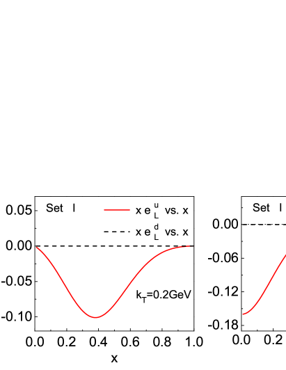
where and represent the vector isoscalar diquark and the vector isovector diquark , respectively, and , and are the parameters of the model. These parameters as well as the mass parameters (such as the diquark masses , cut-off parameters ) are fitted from the ZEUS unpolarized parton distribution functions zeus and GRSV01 polarized parton distribution functions grsv01 . We combine Eqs. (9), (10), (15), and (16) to obtain the Set I distributions and with and . For the strong coupling appearing in the expressions for , we choose . In the left panels of Figs. 1 and 2, we plot the -dependence (at ) of the functions and timed with for and quarks in Set I. We also plot the -dependence (at ) of the distributions in the right panels of Figs. 1 and 2.

Different from Eq. (20), another kind of flavor separation has been employed previously Jakob:1997npa ; Bacchetta:plb578 :
| (21) |
where the coefficients , and in front of are obtained from the SU(4) spin-flavor symmetry of the proton wave function. In this model, the mass parameters for different types of vector diquarks are the same, and we apply the values for the parameters from Ref. Bacchetta:plb578 . Using the relation (21), together with the expressions (9), (10), (19) and (18) , we obtain another set of TMD distributions, which we denote as Set II distributions. The corresponding numerical results are plotted in Figs. 3 and 4.


Comparing Fig. 1 with Fig. 3 and Fig. 2 with Fig. 4, we can see that the sizes of the TMD distributions in Set I are different from those in Set II. In both sets, the signs of and turn to be negative in the specified kinematics ( and GeV). Also, the size of the T-even distribution is generally larger than that of the T-odd distribution . This is understandable since T-odd distributions are yielded from the higher order expansion of gauge link. The distribution has also been calculated Avakian:2010br in the Bag model. We find that the tendency of the dependence of in our calculation agrees with the result in Ref. Avakian:2010br , that is, there is a node in the intermediate region. This behavior may be explained by the so called Lorentz invariance relation Avakian:2010br ; Mulders:1995dh ; Teckentrup:2009tk . We also point out that our result for agrees with the time reversal constraint for distributions .
III Predictions on the asymmetry for charged and neutral pions in polarized SIDIS
In this section, we perform phenomenological analysis on the asymmetry for pions in SIDIS:
| (22) |
Here the arrow denotes the longitudinally polarization of the beam or proton target, and stand for the momenta of the incoming and outgoing leptons, and and denote the momenta of the target nucleon and the final-state hadron, respectively. The kinematics of SIDIS can be expressed by the following invariant variables
| (23) |
with the momentum of the virtual photon, and the invariant mass of the hadronic final state. The reference frame adopted in this work is shown in Fig. 5, in which the momentum of the virtual photon is along the axis, and the longitudinal polarization of the target is along the opposite direction of axis. Thus, we will not consider the contribution from the transverse component of the polarization, which involves the TMD distribution . In this frame, the transverse momentum of the final hadron with respect to the fragmenting quark is denoted by , and the azimuthal angle of the hadron around the virtual photon is defined as .

The differential cross section of SIDIS by scattering a longitudinally polarized lepton beam off a longitudinally polarized target can be expressed as Bacchetta:0611265
| (24) |
here and are the spin-averaged and spin-dependent structure functions, respectively, and the ratio of the longitudinal and transverse photon flux is defined by . The ellipsis stands for the leading-twist double-spin asymmetry Anselmino:2006yc ; Lu:2012ez which will not be analyzed in this work.

By exploiting the notation
| (25) |
we express the structure functions and as Bacchetta:0611265
| (26) | ||||
| (27) |
Here, we introduce the unit vector and use denote the mass of the final hadron. As we restrict our scope on the role of the twist-3 distributions in , in Eq. (27) we have suppressed the terms containing the twist-3 fragmentation functions and .
The asymmetry as a function of can be cast into
| (28) |
where the kinematical factor is defined as
| (29) |
In a similar way, we can define the -dependent and the -dependent asymmetries.


In order to estimate the numerical results of , we apply the model results of and obtained in the previous section . As for the Collins function appearing in Eq. (27), we adopt the parametrization (the standard set) from Ref. Anselmino:2013vqa . To obtain the Collins function for neutral pion, we employ the following isospin relation:
| (30) |
For the TMD fragmentation function , which couples with the distribution , we assume its dependence has a Gaussian form
| (31) |
where is the integrated fragmentation function , for which we adopt the leading order set of the DSS parametrization Florian:2007prd . For the Gaussian width , we choose its numerical value as GeV2, following the fitted result in Ref. Anselmino:2005prd . Finally, in our calculation, we consider the kinematical constraints on the intrinsic transverse momentum of the initial quarks given in Ref. Boglione:2011 .
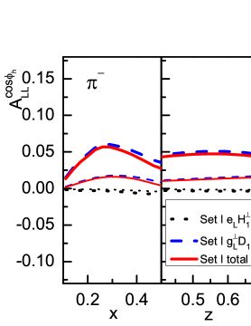
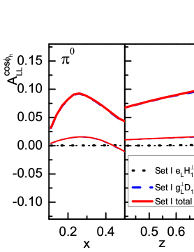
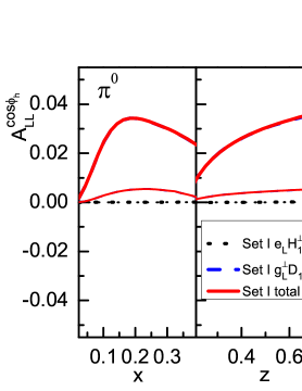
We apply the following kinematics to estimate the asymmetry at CLAS:
In the left, central, and right panels of Fig. 6, we plot the asymmetry for , and as functions of , , and . The thick and thin curves correspond to the asymmetries that calculated from the TMD distributions of Set I and Set II, respectively. The dotted curves show the asymmetries contributed by , the dashed curves show those contributed by , while the solid curves denote the total contribution. We find that the asymmetries calculated from both sets of TMD distributions are positive for all three pions. Also, It is clear that the asymmetries contributed by the T-even distribution dominate, and those contributed by are almost negligible. The asymmetries calculated from Set I TMD distributions are about 5 to 10 percent in magnitude, and are several times larger than those from Set II distributions.
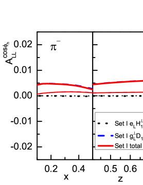
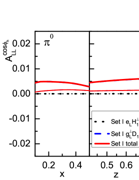
Using the two sets of TMD distributions, we also predict the asymmetry at HERMES with a 27.6 GeV positron beam off a proton target Airapetian:2005jc :
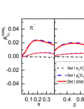
and at COMPASS with a 160 GeV muon beam scattered off a deuteron target Alekseev:2010dm :
In Figs. 7 and 8, we show our prediction on the asymmetry for charged and neutral pions at HERMES and COMPASS, respectively. We find that the asymmetry at HERMES is smaller than that at CLAS. Again, the T-even distribution gives the dominant contribution. The asymmetries for all pions from the two sets of TMD distributions at COMPASS are consistent with zero (less than 0.5%).
IV Conclusion
In this work, we investigated the azimuthal asymmetry in the double longitudinally polarized SIDIS. Particularly, we focused on the role of the genuine twist-3 TMD distributions and ignored the contribution from the twist-3 fragmentation functions. To give a quantitative estimate on the asymmetry for different pions, we calculated and of the valence quarks within the framework of spectator model. We considered two different forms for the propagator of the vector diquark as well as different choices on the flavor separation to obtain two sets of TMD distributions, which were used to predict the asymmetry for , and at the kinematics of CLAS, HERMES and COMPASS. We found that the asymmetries from both sets of TMD distributions are sizable at CLAS, while at HERMES only the asymmetry from the distribution of Set I is measurable. Therefore, it would be feasible to access the asymmetry at least at CLAS. We also found that the predicted asymmetries are positive for all the pions. This is different from the estimate Anselmino:2006yc based on the Cahn effect, which predicts negative asymmetries for pions, although the magnitude of the asymmetry in our calculation is consistent with the result in Ref. Anselmino:2006yc . A positive asymmetry thus can be viewed as a clear signal of dynamical twist-3 effect that is different from the Cahn effect. Furthermore, our study shows that the main contribution to the asymmetry is from the T-even distribution , while the contribution from the T-odd distribution almost vanishes. Future experimental data on the azimuthal asymmetry in the double longitudinally polarized reaction will clarify the role of the twist-3 TMD distributions.
Acknowledgements
This work is partially supported by the National Natural Science Foundation of China (Grants No. 11120101004, No. 11005018, and No. 11035003), and by the Qing Lan Project (China). W.M. is supported by the Scientific Research Foundation of the Graduate School of SEU (Grant No. YBJJ1336).
References
- (1) R.N. Cahn, Phys. Lett. B 78, 269 (1978); R.N. Cahn, Phys. Rev. D 40, 3107 (1989).
- (2) J. Ashman et al. [European Muon Collaboration], Z. Phys. C 52, 361 (1991).
- (3) J. J. Aubert et al. [European Muon Collaboration], Phys. Lett. B 130, 118 (1983).
- (4) M. Arneodo et al., Z. Phys. C 34, 277 (1987).
- (5) M. R. Adams et al. [E665 Collaboration], Phys. Rev. D 48, 5057 (1993).
- (6) H. Mkrtchyan, P. E. Bosted, G. S. Adams, A. Ahmidouch, T. Angelescu, J. Arrington, R. Asaturyan and O. K. Baker et al., Phys. Lett. B 665, 20 (2008) [arXiv:0709.3020 [hep-ph]].
- (7) M. Osipenko et al. [CLAS Collaboration], Phys. Rev. D 80, 032004 (2009) [arXiv:0809.1153 [hep-ex]].
- (8) A. Airapetian et al. [HERMES Collaboration], Phys. Rev. D 87, no. 1, 012010 (2013) [arXiv:1204.4161 [hep-ex]].
- (9) C. Adolph et al. (COMPASS Collaboration), Nucl. Phys. B886, 311 (2014).
- (10) M. Anselmino, M. Boglione, U. D’Alesio, A. Kotzinian, F. Murgia, and A. Prokudin, Phys. Rev. D 71, 074006 (2005).
- (11) P. Schweitzer, T. Teckentrup and A. Metz, Phys. Rev. D 81, 094019 (2010) [arXiv:1003.2190 [hep-ph]].
- (12) M. Boglione, S. Melis, and A. Prokudin, Phys. Rev. D 84, 034033 (2011).
- (13) J. S. Conway, et al., Phys. Rev. D 39, 92 (1989).
- (14) M. Anselmino, A. Efremov, A. Kotzinian and B. Parsamyan, Phys. Rev. D 74, 074015 (2006).
- (15) A. Bacchetta, M. Diehl, K. Goeke, A. Metz, P.J. Mulders, and M. Schlegel, J. High Energy Phys. 02 (2007) 093.
- (16) P. J. Mulders and R. D. Tangerman, Nucl. Phys. B 461, 197 (1996) [Erratum-ibid. B 484, 538 (1997)] [hep-ph/9510301].
- (17) J.C. Collins, Nucl. Phys. B396, 161 (1993).
- (18) A. Airapetian et al. (HERMES Collaboration), Phys. Lett. B622, 14 (2005).
- (19) A. Airapetian et al. (HERMES Collaboration), Phys. Lett. B 648, 164 (2007).
- (20) M.G. Alekseev et al. (COMPASS Collaboration), Eur. Phys. J. C 70, 39 (2010)
- (21) M. Aghasyan et al., Phys. Lett. B 704, 397 (2011).
- (22) W. Gohn et al. [CLAS Collaboration], Phys. Rev. D 89, no. 7, 072011 (2014) [arXiv:1402.4097 [hep-ex]].
- (23) B. Parsamyan, EPJ Web Conf. 85, 02019 (2015) [arXiv:1411.1568 [hep-ex]].
- (24) A. Metz and M. Schlegel, Eur. Phys. J. A 22, 489 (2004).
- (25) A. Bacchetta, P. J. Mulders and F. Pijlman, Phys. Lett. B 595, 309 (2004) [hep-ph/0405154].
- (26) W. Mao and Z. Lu, Phys. Rev. D 87, 014012 (2013).
- (27) Y.-k. Song, J.-h. Gao, Z.-t. Liang, and X.-N. Wang, Phys. Rev. D 89, 014005 (2014).
- (28) Y.-k. Song, Z.-t. Liang, and X.-N. Wang, Phys. Rev. D 89, 117501 (2014).
- (29) Z. Lu, Phys. Rev. D 90, 014037 (2014).
- (30) W. Mao, Z. Lu, and B.-Q. Ma, Phys. Rev. D 90, 014048 (2014).
- (31) R. Jakob, P.J. Mulders, and J. Rodrigues, Nucl. Phys. A626, 937 (1997).
- (32) S.J. Brodsky, D.S. Hwang, B.-Q. Ma, and I. Schmidt, Nucl. Phys. B593, 311 (2001).
- (33) S.J. Brodsky, D.S. Hwang, and I. Schmidt, Phys. Lett. B 530, 99 (2002).
- (34) X. Ji and F. Yuan, Phys. Lett. B 543, 66 (2002).
- (35) A. Bacchetta, A. Schäfer, and J.J Yang, Phys. Lett. B 578, 109 (2004).
- (36) L.P. Gamberg, D.S. Hwang, A. Metz, M. Schlegel, Phys. Lett. B 639, 508-512 (2006).
- (37) A. Bacchetta, F. Conti, and M. Radici, Phys. Rev. D 78, 074010 (2008).
- (38) Z. Lu and I. Schmidt, Phys. Lett. B 712, 451 (2012).
- (39) K. Goeke, A. Metz, and M. Schlegel, Phys. Lett. B 618, 90 (2005).
- (40) J.C. Collins, Phys. Lett. B 536, 43 (2002).
- (41) S. Chekanov et al. (ZEUS Collaboration), Phys. Rev. D 67, 012007 (2003).
- (42) M. Glück, E. Reya, M. Stratmann, and W. Vogelsang, Phys. Rev. D 63, 094005 (2001).
- (43) H. Avakian, A. V. Efremov, P. Schweitzer and F. Yuan, Phys. Rev. D 81, 074035 (2010) [arXiv:1001.5467 [hep-ph]].
- (44) T. Teckentrup, A. Metz and P. Schweitzer, Mod. Phys. Lett. A 24 (2009) 2950 [arXiv:0910.2567 [hep-ph]].
- (45) Z. Lu and B. Q. Ma, Phys. Rev. D 87, no. 3, 034037 (2013) [arXiv:1212.6864 [hep-ph]].
- (46) M. Anselmino, M. Boglione, U. D’Alesio, S. Melis, F. Murgia and A. Prokudin, Phys. Rev. D 87, 094019 (2013).
- (47) D. de Florian, R. Sassot, and M. Stratmann, Phys. Rev. D 75, 114010 (2007).