Unraveling Quantum Annealers using Classical Hardness
Abstract
Recent advances in quantum technology have led to the development and manufacturing of experimental programmable quantum annealing optimizers that contain hundreds of quantum bits. These optimizers, named ‘D-Wave’ chips, promise to solve practical optimization problems potentially faster than conventional ‘classical’ computers. Attempts to quantify the quantum nature of these chips have been met with both excitement and skepticism but have also brought up numerous fundamental questions pertaining to the distinguishability of quantum annealers from their classical thermal counterparts. Here, we propose a general method aimed at answering these, and apply it to experimentally study the D-Wave chip. Inspired by spin-glass theory, we generate optimization problems with a wide spectrum of ‘classical hardness’, which we also define. By investigating the chip’s response to classical hardness, we surprisingly find that the chip’s performance scales unfavorably as compared to several analogous classical algorithms. We detect, quantify and discuss purely classical effects that possibly mask the quantum behavior of the chip.
I Introduction
Interest in quantum computing originates in the potential of quantum computers to solve certain computational problems much faster than is possible classically, due to the unique properties of Quantum Mechanics Shor (1994); Grover (1997). The implications of having at our disposal reliable quantum computing devices are obviously tremendous. The actual implementation of quantum computing devices is however hindered by many challenging difficulties, the most prominent being the control or removal of quantum decoherence Schlosshauer (2004). In the past few years, quantum technology has matured to the point where limited, task-specific, non-universal quantum devices such as quantum communication systems, quantum random number generators and quantum simulators, are being built, possessing capabilities that exceed those of corresponding classical computers.
Recently, a programmable quantum annealing machine, known as the D-Wave chip Johnson et al. (2011), has been built whose goal is to minimize the cost functions of classically-hard optimization problems presumably by adiabatically quenching quantum fluctuations. If found useful, the chip could be regarded as a prototype for general-purpose quantum optimizers, due to the broad range of hard theoretical and practical problems that may be encoded on it.
The capabilities, performance and underlying physical mechanism driving the D-Wave chip have generated fair amounts of curiosity, interest, debate and controversy within the Quantum Computing community and beyond, as to the true nature of the device and its potential to exhibit clear “quantum signatures”. While some studies have concluded that the behavior of the chip is consistent with quantum open-system Lindbladian dynamics Albash et al. (2012) or indirectly observed entanglement Lanting et al. (2014), other studies contesting these Smolin and Smith ; Shin et al. (2014) pointed to the existence of simple, purely classical, models capable of exhibiting the main characteristics of the chip.
Nonetheless, the debate around the quantum nature of the chip has raised several fundamental questions pertaining to the manner in which quantum devices should be characterized in the absence of clear practical “signatures” such as (quantum) speedups Ronnow et al. (2014); Boixo et al. (2014). Since quantum annealers are meant to utilize an altogether different mechanism for solving optimization problems than traditional classical devices, methods for quantifying this difference are expected to serve as important theoretical tools while also having vast practical implications.
Here, we propose a method that partly solves the above question by providing a technique to characterize, or measure, the “classicality” of quantum annealers. This is done by studying the algorithmic performance of quantum annealers on sets of optimization problems possessing quantifiable, varying degrees of “thermal” or “classical” hardness, which we also define for this purpose. To illustrate the potential of the proposed technique, we apply it to the experimental quantum annealing optimizer, the D-Wave Two (DW2) chip.
We observe several distinctive phenomena that reveal a strong correlation between the performance of the chip and classical hardness: i) The D-Wave chip’s typical time-to-solution () as a function of classical hardness scales differently, in fact worse, than that of thermal classical algorithms. Specifically, we find that the chip does very poorly on problem instances exhibiting a phenomenon known as “temperature chaos”. ii) Fluctuations in success probability between programming cycles become larger with increasing hardness, pointing to the fact that encoding errors become more pronounced and destructive with increasing hardness. iii) The success probabilities obtained from harder instances are affected more than easy instances by changes in the duration of the anneals.
Analyzing the above findings, we identify two major probable causes for the chip’s observed “sub-classical” performance, namely i) that its temperature may not be low enough, and ii) that encoding errors become more pronounced with increasing hardness. We further offer experiments and simulations designed to detect and subsequently rectify these so as to enhance the chip’s capabilities.
II Classical Hardness, temperature chaos and parallel tempering
In order to study the manner in which the performance of quantum annealers correlates with ‘classical hardness’, it is important to first accurately establish the meaning of classical hardness. For that purpose, we refer to spin-glass theory Young (1998), which deals with spin glasses— disordered, frustrated spin systems that may be viewed as prototypical classically-hard (also called NP-hard) optimization problems, that are so challenging that specialized hardware has been built to simulate them Belletti et al. (2008, 2009); Baity-Jesi et al. (2014).
Currently, the (classical) method of choice to study general spin-glass problems is Parallel Tempering (PT, also known as ‘exchange Monte Carlo’) Hukushima and Nemoto (1996); Marinari (1998). PT is a refinement of the celebrated yet somewhat outdated Simulated Annealing algorithm Kirkpatrick et al. (1983), that finds optimal assignments (i.e., the ground-state configurations) of given discrete-variable cost functions. It is therefore only natural to make use of the performance of PT to characterize and quantify classical hardness.
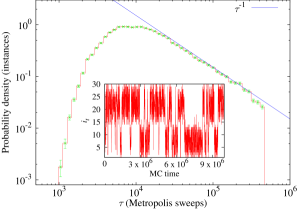
In PT simulations, one considers copies of an -spin system at temperatures , where each copy undergoes Metropolis spin-flip updates independently of other copies. In addition, copies with neighboring temperatures regularly attempt to swap their temperatures with probabilities that satisfy detailed balance Sokal (1997). In this way, each copy performs a temperature random-walk (see inset of Fig 1). At high temperatures, free-energy barriers are easily overcome, allowing for a global exploration of configuration space. At lower temperatures on the other hand, the local minima are explored in more detail. A ‘healthy’ PT simulation requires an unimpeded temperature flow: The total length of the simulation should be longer than the temperature ‘mixing time’ Fernandez et al. (2009a); Alvarez Baños et al. (2010). The time may be thought of as the average time it takes each copy to fully traverse the temperature mesh, indicating equilibration of the simulation. Therefore, instances with large are harder to equilibrate, which motivates our definition of the mixing time as the classical hardness of a given instance.
Despite the popularity of PT, it has also become apparent that not all the spin-glass problems can be efficiently solved by the algorithm Alvarez Baños et al. (2010); Fernandez et al. (2013). The reason is a phenomenon that has become known as Temperature Chaos (TC). TC McKay et al. (1982); Bray and Moore (1987); Banavar and Bray (1987); Kondor (1989); Kondor and Végsö (1993); Billoire and Marinari (2000); Rizzo (2001); Mulet et al. (2001); Billoire and Marinari (2002); Krzakala and Martin (2002); Rizzo and Crisanti (2003); Parisi and Rizzo (2010); Sasaki et al. (2005); Katzgraber and Krzakala (2007); Fernandez et al. (2013); Billoire (2014) consists of a sequence of first-order phase transitions that a given spin-glass instance experiences upon lowering its temperature, whereby the dominant configurations minimizing the free energy above the critical temperatures are vastly different than those below them (Fig. 2 depicts such a phase that is ‘rounded’ due to the finite size of the system). A given instance may experience zero, one or more transitions at random temperatures, making the study of TC excruciatingly difficult Sasaki et al. (2005); Katzgraber and Krzakala (2007); Fernandez et al. (2013); Billoire (2014). Such TC transitions hinder the PT temperature flow, significantly prolonging the mixing time . In practice Fernandez et al. (2013), it is found that for small systems the large majority of the instances do not suffer any TC transitions and are ‘easy’ (i.e., they are characterized by short mixing times). However, for a minor fraction of them, turns out to be inordinately large. Moreover, the larger the system is, the larger the fraction of long- samples becomes. In the large limit, these are the short- samples that become exponentially rare in Rizzo and Crisanti (2003); Fernandez et al. (2013). This provides further motivation for studying TC instances of optimization problems on moderately small experimental devices (even if they are rare).

III Temperature chaos and quantum annealers
With the advent of quantum annealers, which presumably offer non-thermal mechanisms for finding ground states, it has become only natural to ask whether quantum annealers can be used to solve ‘TC-ridden’ optimization problems faster than classical techniques such as PT. In this context, the question of how the performance of quantum annealers depends on the ‘classical hardness’ becomes of fundamental interest: If indeed quantum annealers exploit quantum phenomena such as tunneling to traverse energy barriers, one may hope that they will not be as sensitive to the thermal hardness (as defined above) of the optimization problems they solve. As we shall see next, having a practical definition for classical hardness allows us to address the above questions directly.
To illustrate this, in what follows we apply the ideas introduced above to the DW2 quantum annealing optimizer in order to infer its degree of ‘classicality’. We accomplish this by first generating an ensemble of instances that are directly embeddable on the DW2 ‘Chimera’ architecture [the reader is referred to Appendix C for a detailed description of the Chimera lattice and the D-wave chip and its properties]. The chip on which we perform our study is an array of 512 superconducting flux qubits of which only 476 are functional, operating at a temperature of mK. The DW2 chip is designed to solve a very specific type of problems, namely, Ising-type optimization problems, by adiabatically transitioning the system Hamiltonian from an initial transverse-field Hamiltonian to a final classical programmable cost function of a typical spin glass. The latter is given by the Ising Hamiltonian:
| (1) |
The Ising spins, are the variables to be optimized over, and the sets and are programmable parameters of the cost function. Here, denotes a sum over all the active edges of the Chimera graph. For simplicity, we conduct our study on randomly-generated problem instances with and random, equiprobable couplings (in our energy units ).
Initially, it is not clear whether the task of finding thermally-hard instances on the Chimera is feasible. While on the one hand TC has been observed in spin-glasses on the square lattice Thomas et al. (2011), which has the same spatial dimension, , as the Chimera Katzgraber et al. (2014), it has also been found that typical Chimera-embeddable instances are easy to solve Ronnow et al. (2014); Boixo et al. (2014); Katzgraber et al. (2014). As discussed above, system size plays a significant role in this context, as an -spin Chimera may simply be too small to have instances exhibiting TC.111For instance, on the square lattice one needs to reach spins for TC to be the rule rather than the exception Thomas et al. (2011). Taking a brute-force approach to resolve this issue, we generated random problem instances (each characterized by a different set of ), analyzing each one by running them on a state-of-the-art PT algorithm until equilibration was reached (Appendix B). This allowed for the calculation of the instances’ classical hardness, namely their temperature mixing times (for more details, see Appendix A, below). The resulting distribution of over the instances is shown in Fig. 1. While most instances equilibrate rather quickly (after some MC steps), we find that the distribution has a ‘tail’ of hard samples with revealing that hard instances, although rare, do exist (we estimate that 2 samples in have ).
To study the DW2 chip, we grouped together instances with similar classical hardness, i.e., similar mixing times, for and . For each such ‘generation’ of , we randomly picked 100 representative instances for running on the chip (only 14 instances with were found). As a convergence test of PT on the selected instances, we verified that the ground-state energies reached by PT are the true ones by means of an exact solver.
At the purely classical level, we found, as anticipated Fernandez et al. (2013), that classically hard instances differ from easy instances from a thermodynamic point of view as well. Specifically, large instances were found to exhibit sharp changes in the average energy at random critical temperatures, consistently with the occurrence of TC (see Fig. 2). For such instances, the true ground states are present during the simulations only below the TC critical temperatures. As the inset shows, the larger is, the lower these critical temperatures typically are. Furthermore, classically-hard instances were found to differ from easier ones in terms of their energy landscape: While for easy instances minimally-excited states typically reside only a few spin flips away from ground state configurations, for classically hard instances, this is not the case (see Appendix B).
IV Classicality of the “D-Wave Two” chip
Having sorted and analyzed the randomly-generated instances, we turned to experimentally test the performance of the D-Wave chip on these (for details see Appendix A and C.4). Our experiments consisted of programming the chip to solve each of the 414 instances over a dense mesh of annealing times in the available range of . The number of attempts, or anneals, that each instance was run for each choice of ranged between and . By calculating the success probability of the annealer for each instance and annealing time, a typical time-to-solution was obtained for each hardness-group, or ‘-generation’ (see Appendix A). Interestingly, we found that for easy samples () the success probability depends only marginally on , pointing to the annealer reaching its asymptotic performance on these. As instances become harder, the sensitivity of success probability to increases significantly. Nonetheless, for all hardness groups, the typical is found to be shortest at the minimally-allowed annealing time of s (see Appendix C.4 for a more detailed discussion).
The main results of our investigation are summarized in Fig. 3 depicting the typical time to solution of the DW2 chip (averaged over instances of same hardness groups, see Appendix A) as a function of classical hardness, or ‘-generation’. As is clear from the figure, the performance of the chip was found to correlate strongly with the ‘thermal hardness’ parameter, indicating the significant role thermal hardness plays in the annealing process. Interestingly, the chip’s response was found to be affected by thermal hardness even more than PT, i.e., more strongly than the classical thermal response: While for PT the time-to-solution scales as , the scaling of the D-Wave chip was found to scale as , with . This scaling is rather surprising given that for quantum annealers to perform better than classical ones, one would expect these to be less susceptible to thermal hardness, not more. Nonetheless, it is clear that the notion of classical hardness is very relevant to the D-wave chip.

To complete the picture, we have also tested our instances on the Hamze-de Freitas-Selby (HFS) algorithm Hamze and de Freitas (2004); Selby (2014), which is the fastest classical algorithm to date for Chimera-type instances. Even though the HFS algorithm is a ‘non-thermal’ algorithm (i.e., it does not make use of a temperature parameter), we have found the concept of classical hardness to be very relevant here as well. For the HFS algorithm, we find a scaling of with , implying that the algorithm is significantly less susceptible to thermal hardness than PT.222It is worth pointing out that the typical runtime for the HFS algorithm on the hardest, , group problems was found to be s on an Intel Xeon CPU E5462 @ 2.80GHz, which to our knowledge makes these the hardest known Chimera-type instances to date.
V Analysis of findings
The above somewhat less-than-favorable performance of the experimental D-wave chip on thermally-hard problems is not necessarily a manifestation of the intrinsic limitations of quantum annealing, i.e., it does not necessarily imply that the ‘quantum landscape’ of the tested problems is harder to traverse than the classical one (although this may sometimes be the case Hen and Young (2011); Farhi et al. (2012)). A careful analysis of the results suggests in fact at least two different more probable ‘classical’ causes for the chip’s performance.
First, as already discussed above and succinctly captured in Fig. 2, temperature is expected to play a key role in DW2 success on instances exhibiting TC. This is because for these, the ground state configurations minimize the free energy only below the lowest critical TC temperature. Even though the working temperature of the DW2 chip is rather low, namely mK, the crucial figure of merit is the ratio of coupling to temperature [recall Eq. (1)]. Although the nominal value for the chip is , any inhomogeneity of the temperature across the chip may render the ratio higher kin , possibly driving it above typical TC critical temperatures.333We refer to the physical temperature of the chip. However, non-equilibrium systems (e.g., supercooled liquids or glasses) can be characterized by two temperatures Cugliandolo et al. (1997): On the one hand, the physical temperature which rules fast degrees of freedom that equilibrate. On the other hand, the ‘effective’ temperature refers to slow degrees of freedom that remain out of equilibrium. We are currently investigating whether or not the DW2 chip can analogously be characterized by two such temperatures.
Another possible cause for the above scaling may be due to the analog nature of the chip. The programming of the coupling parameters and magnetic fields is prone to statistical and systematic errors (also referred to as intrinsic control errors, or ICE). The couplings actually encoded in DW2 are , where is a random error (, according to the chip’s manufacturer). Unfortunately, even tiny changes in coupling values are known to potentially change the ground-state configurations of spin glasses in a dramatic manner Nifle and Hilhorst (1992); Ney-Nifle (1998); Krzakala and Bouchaud (2005); Katzgraber and Krzakala (2007). We refer to this effect as ‘coupling chaos’ (or -chaos, for short). For an -bit system, -chaos seems to become significant for . Empirically Krzakala and Bouchaud (2005); Katzgraber and Krzakala (2007) , being the spatial dimension of the system. Note, however, that these estimates refer only to typical instances and small whereas the assessment of the effects of -chaos on thermally-hard instances remains an important open problem for classical spin glasses.
Here, we empirically quantify the effects of -chaos by taking advantage
of the many programming cycles and gauge choices each instance has
been annealed with (typically between 200 and 2000). Calculating a success probability for each cycle, we compute the probability distribution of
over different cycles for each instance Fernandez et al. (2013); Billoire (2014). We find that while
for some instances is essentially insensitive to programming
errors, for other instances (even within the same thermal hardness
group), varies significantly, spanning several orders of
magnitude. This is illustrated in Fig. 4 which
presents some results based on a straightforward percentile analysis
of these distributions. For instance #1 in the figure,
the th percentile probability is , whereas
the probability at the th percentile is
. Hence the ratio
is close to one. Conversely, for instance #35, the values are ,
and the ratio is , i.e., the
success probability drops by an order of magnitude. The inset of
Fig. 4 shows the typical ratio as a function
of classical hardness, demonstrating the strong correlation between
thermal hardness and the devastating effects of -chaos caused by ICE, namely that
the larger is, the more probable it is to find instances for
which varies wildly between programming cycles.

VI Discussion
We have devised a method for quantifying the ‘classicality’ of quantum annealers by studying their performance on sets of instances characterized by different degrees of thermal hardness, which we have defined for that purpose as the mixing (or equilibration) time of classical thermal algorithms (namely, PT) on these. We find that the 2D-like Chimera architecture used in the D-Wave chips does give rise to thermally very-hard, albeit rare, instances. Specifically, we have found samples that exhibit temperature chaos, and as a such have very long mixing times, i.e., they are classically exceptionally hard to solve.
Applying our method to an experimental quantum annealing optimizer, the DW2 chip, we have found that its performance is more susceptible to changes in thermal hardness than classical algorithms. This is in contrast with the performance of the best-known state-of-the-art classical solver on Chimera graphs, the ‘non-thermal’ HFS algorithm, which scales (unsurprisingly) better. Our results are not meant to suggest that the DW2 chip is not a quantum annealer, but rather that its quantum properties may be significantly masked by much-undesired classical effects.
We have identified and quantified two probable causes for the observed behavior: A possibly too high temperature, or more probably, -chaos, the random errors stemming from the digital-to-analog conversion in the programming of the coupling parameters. One may hope that the scaling of current DW2 chips would significantly improve if one or both of the above issues are resolved. Clearly, lowering the temperature of the chip and/or reducing the error involved in the programming of its parameters are both technologically very ambitious goals, in which case error correcting techniques may prove very useful Pudenz et al. (2014). We believe that quantum Monte Carlo simulations of the device will be instrumental in the understanding of the roles that temperature and magnitude of programming errors play in the performance of the chip (and of its classical counterparts). In turn, this will help sharpening the most pressing technological challenges facing the fabrication of these and other future quantum optimizing devices, paving the way to obtaining a long-awaited insights as to the difference between quantum and classical hardness in the context of optimization. We are currently pursuing these approaches.
Acknowledgments
We thank Luis Antonio Fernández and David Yllanes for providing us with their analysis program for the PT correlation function. We also thank Marco Baity-Jesi for helping us to prepare the figures.
We are indebted to Mohammad Amin, Luis Antonio Fernández, Enzo Marinari, Denis Navarro, Giorgio Parisi, Federico Ricci-Tersenghi and Juan Jesús Ruiz-Lorenzo for discussions.
We thank Luis Antonio Fernández, Daniel Lidar, Felipe LLanes-Estrada, David Yllanes and Peter Young for their reading of a preliminary version of the manuscript.
We thank D-Wave Systems Inc. for granting us access to the chip.
We acknowledge the use of algorithms and source code for a classic solver, devised and written by Alex Selby, available for public usage at https://github.com/alex1770/QUBO-Chimera.
IH acknowledges support by ARO grant number W911NF-12-1-0523. VMM was supported by MINECO (Spain) through research contract No FIS2012-35719-C02.
Appendix A Methods
Computation of the mixing time .— Because we follow Ref. Alvarez Baños et al. (2010), we just briefly summarize here the main steps of the procedure. Considering one of the system copies in the PT simulation, let us denote the temperature of copy at Monte Carlo time by , where (see inset of Fig. 1). At equilibrium, the probability distribution for is uniform (namely, ) hence the exact expectation value of is . From the general theory of Markov Chain Monte Carlo Sokal (1997), it follows that the equilibrium time-correlation function may be written as a sum of exponentially decaying terms:
The mixing time is the largest ‘eigen-time’
. We compute numerically the correlation function
and fit it to the decay of two exponential
functions (so we extract the dominant time scale and a
sub-leading time scale). The procedure is described in full in Ref. Alvarez Baños et al. (2010).
D-wave data acquisition and analysis.—
Data acquisition:
In what follows we briefly summarize the steps of the experimental setup and data acquisition for the anneals performed on the 414 randomly-generated instances in the various thermal-hardness groups.
-
1.
The couplings of each of the 414 instances have been encoded onto the D-Wave chip using many different choices of annealing times in the allowed range of s s.
-
2.
For each instance and each choice of the following process has been repeated hundreds to thousands of times:
-
(a)
First, a random ‘gauge’ has been chosen for the instance. A gauge transformation does not change the properties of the optimization problem but has some effect on the performance of the chip which follows from the imperfections of the device that break the gauge symmetry. The different gauges are applied by transforming the original instance , , to the original cost function Eq. (1). The above gauge transformations correspond to the change in configuration spin values. Here, the gauge parameters were chosen randomly.
-
(b)
The chip was then programmed with the gauge-transformed instance (inevitably adding programming bias errors, as mentioned in the main text).
-
(c)
The instance was then solved, or annealed, times within the programming cycle/with the chosen gauge. We chose , the maximally allowed amount.
-
(d)
After the anneals were performed, the number of successes , i.e., the number of times a minimizing configuration had been found, was recorded. The probability of success for the instance, for that particular gauge/programming cycle and annealing time was then estimated as . Note, that in cases where the probability of success is of the order of , the probability will be a rather noisy estimate (see data analysis, below, for a procedure to mitigate this problem).
-
(e)
If the prefixed number of cycles for the current instance and has not been reached, return to (2a) and choose a new gauge.
-
(a)
Data analysis and time-to-solution estimates:
The analysis of the data acquisition process described above proceeded as follows.
-
1.
For each instance and each annealing time, the total number of hits was calculated, where sums over all the gauge/programming cycles. Denoting as the total number of annealing attempts, the probability of success for any particular instance and anneal time was then calculated as .
-
2.
The above probability was then converted into an average time-to-solution for that instance and according to , where the special case of designates an estimate of an infinite , where in practice the true probability lies below the resolution threshold of .
-
3.
A typical runtime for a hardness group was then obtained by taking the median over all minimal values of all the instances in the group.
Appendix B Instance generation and analysis
B.1 The Parallel Tempering simulations
We briefly outline the technical details of the Parallel Tempering (PT) simulations and subsequent analysis performed on the randomly generated instances. The reader is referred to Ref. Alvarez Baños et al. (2010) for further details.
To run the simulations, we employed multi-spin coding Newman and Barkema (1999), a simple yet efficient form of parallel computation, that allows the simultaneous simulations of a large number of problem instances. The name multi-spin follows from the fact that our dynamic variables are binary, , and thus can be coded in a single bit. Hence, one may code the -th spin corresponding to independent instances in a single -bit computer word. Using streaming extensions, can be as large as , nowadays.444Simulations were run on a standard Intel(R) Xeon(R) processors (E5-2690 0 @ 2.90GHz). The advantages of simulating in parallel 256 instances are obvious, if we want to study a huge number of problems in our quest for these rare instances displaying Temperature Chaos. In fact, we have simulated a total of problem instances.
The temperature grid of the PT simulations consisted of temperatures. Temperatures with indices were evenly distributed in the range , while lower temperatures in the range (indices ) have been added in order to detect temperature chaos effects.555In our simulations, the minimal temperature value corresponds effectively to zero temperature. This follows from the minimal energy gap of our instances being together with our use of a 64-bit (pseudo) random-number generator Fernandez et al. (2009b). Setting such that it obeys , our Metropolis simulations at effectively become equivalent to simulations. Ergodicity was maintained by the temperature-swap part of the PT.
For each instance, we ran four independent simulations (i.e., four replicas) per temperature, where an elementary Monte Carlo step consisted of 10 full lattice Metropolis sweeps, followed by a PT temperature swap attempt. Since the Chimera lattice is bipartite, Metropolis sweeps have been carried out on alternating partitions at each step.
The calculation of the mixing time was conducted in three stages, or rounds (see also Ref. Alvarez Baños et al. (2010)). In the first stage, all instances were simulated for a total of elementary Monte Carlo steps (i.e., each system was simulated for full-lattice Metropolis sweep). At the end of each round the mixing time was computed (measured in units of full-lattice Metropolis sweeps). As can also be read off Fig. 1 of the main text, the first-round of simulations was adequate for the equilibration of most instances, namely, for problems of -generations and . The second round of simulations was set to last 10 times longer, consisting of elementary Monte Carlo steps, or full-lattice Metropolis sweeps per system. These longer simulations were reserved only to the hardest instances corresponding to -generations of or larger.666The criterion for selecting the hardest instances to qualify for subsequent rounds of simulations was done by assigning a figure of merit for each instance based on the performance of its system copies. For each of the copies, the fraction of Monte Carlo time spent at the higher-temperatures regions, namely with , was calculated where the figure of merit was chosen to be the smallest of these fractions, which was used as an indication for how trapped the instance is in the low-temperatures region. The 256 worse-scoring instances of these were further simulated for elementary Monte Carlo steps (or full-lattice Metropolis sweeps per system). This simulation lasted 10 days on our fastest CPU [Intel(R) Core(TM) i7-4770K CPU @ 3.50GHz]. From it, we obtained 14 extremely hard problem instances, belonging to -generation .
B.2 Spin-overlap analysis
Here, we briefly extend the analysis of the energy landscapes of thermally-hard problems, initiated in Fig. 2 of the main text. To do so, we make use of the notion of ‘spin-overlap’, which plays a major role in any spin glass investigation (see, e.g., Ref. Young (1998)). The spin overlap between two -spin configurations and is defined as
| (3) |
where is the Hamming distance between the two configurations, i.e., the number of spins by which the two configurations differ. For two identical configurations we get and while for two configurations differing by a global spin flip (i.e., for all ) we have and . Since the instances we study all have , their Hamiltonians possess a global bit-flip symmetry. For any configuration , its spin-reversed configuration has the same energy. We have therefore chosen to consider the more informative measure of the absolute value of the overlap, . In this case, the maximum meaningful Hamming distance between any two configurations is .
We utilized spin overlaps to investigate the energy landscapes of the various instances in the following way. During the PT simulations, 12000 spin configurations of each instance were stored on disk, corresponding to 100 evenly spaced check-points in Monte Carlo time where every check-point contains configurations. Of those, ground-state (GS) configurations777 For a spin-glass, the ground state is typically highly degenerate even in two dimensions Barahona et al. (1982). Empirically, we find that this high-degeneracy is also present on the 2D-like Chimera Katzgraber et al. (2014). and minimally-excited (ES) states were picked out for further analysis. Our analysis consisted of examining the probability distributions of overlaps between (i) randomly chosen GS configurations and randomly chosen ES configurations [GS-ES, solid blue curves in Fig. 5 of Extended Data (ED)] and (ii) pairs of randomly chosen GS configurations (GS-GS, dashed red curves in Fig. 5). Two extremal cases were encountered. For easy instances (Fig. 5–top), the probability density for GS-GS overlaps is very similar to the probability density for GS-ES overlaps. This is expected in cases where ES states are trivially connected to GS states via one spin-flip. Conversely, for hard instances (Fig. 5–bottom), the probability densities for GS-GS overlaps and for GS-ES overlaps differ significantly, indicating that the vast majority of the ES states encountered during the simulations are not trivially connected to typical GS configurations but are rather very distant from them.
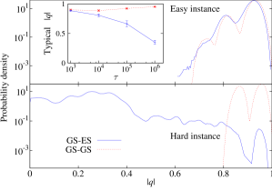
The top and bottom panels of Fig. 5 describe only two representative instances, however the above depiction was also found to be valid in the general case, as is confirmed by calculation of the typical for all the instances in each of the hardness groups.888In order to define a typical , we follow a two-steps procedure. First, we obtain a typical for each instance by computing the median overlap [e.g. for the easy instance in the top panel of Fig. 5 , while for the hard instance in the bottom panel ]. Second, we average over all the instances in a -generation, by computing the median over the instance medians. As the inset of Fig. 5 shows, the harder instances are, the further away minimally excited states are from ground states.
Appendix C The D-Wave Two Chip
C.1 The Chimera
The Chimera graph of the D-Wave Two (DW2) chip used in this study is shown in Fig. 6. The chip is an array of unit cells where each unit cell is a balanced bipartite graph of superconducting flux qubits. In the ideal Chimera graph the degree of each (internal) vertex is . On our chip, only a subset of 476 qubits, is functional. The temperature of the device mK.

The chip is designed to solve a very specific type of problems, namely, Ising-type optimization
problems where the cost function is that of the Ising Hamiltonian [see Eq. (1) of the main text]. The Ising spins,
are the variables to be optimized over and the sets
and are the programmable parameters of the cost
function. In addition, denotes a sum over all
active edges of the Chimera graph.
C.2 The D-Wave Two annealing schedule
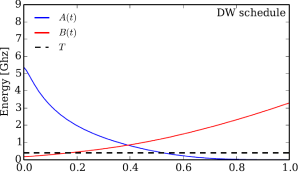
The DW2 performs the annealing by implementing the time-dependent Hamiltonian
| (4) |
with where the allowed range of annealing times , due to engineering restrictions, is between s and s. The annealing schedules and used in the device are shown in Fig. 7. There are four annealing lines, and their synchronization becomes harder for faster annealers. The filtering of the input control lines introduces some additional distortion in the annealing control.
C.3 Gauge averaging on the D-Wave device
Calibration inaccuracies stemming mainly from the digital to analog conversions of the problem parameters, cause the couplings and realized on the DW2 chip to be slightly different from the intended programmed values (with a typical variation). Therefore, instances encoded on the device will be generally different from the intended instances. Additionally, other, more systematic biases exist which cause spins to prefer one orientation over another regardless of the encoded parameters. To neutralize these effects, it is advantageous to perform multiple annealing rounds (or ‘programming cycles’) on the device, where each such cycle corresponds to a different encoding or ‘gauge’ of the same problem instance onto the couplers of the device Ronnow et al. (2014). To realize these different encodings, we use a gauge freedom in realizing the Ising spin glass: for each qubit we can freely define which of the two qubits states corresponds to and . More formally this corresponds to a gauge transformation that changes spins , with and the couplings as and . The simulations are invariant under such a gauge transformation, but due to calibration errors which break the gauge symmetry, the results returned by the DW2 are not.
C.4 Performance of the DW2 chip as a function of annealing time
Since the DW2 chip is a putative quantum annealer, it is only natural to ask how its performance, namely, the typical time-to-solution it yields, depends on annealing time . Ideally, the longer is, the better the performance we expect Kadowaki and Nishimori (1998). However, in practice, decohering interactions with the environment are present which become more pronounced with longer running times of the annealing process. It is therefore plausible to assume that there is an optimal for which is shortest Ronnow et al. (2014).
Analysis of the dependence of success probabilities, or equivalently times to solution, on annealing time is found to be heavily blurred, or masked, by fluctuations in the success probability between different programming cycles. These fluctuations, which become more pronounced for harder instances, stem from the noisy encoding of the instance parameters already discussed above. Any meaningful analysis of the dependence of success probability on annealing time must therefore successfully average out these effects therefore requires many rounds of anneals. Unfortunately (see data acquisition in Appendix A) the number of annealing attempts for a given DW2 programming cycle is proportional to , ranging from , to As a consequence, the minimal success probability that can be measured from a programming cycle is just . While this limitation is not serious for easy instances (i.e., those of the group), for hard instances a typical success probability is much smaller than . This problem can be alleviated by running the DW2 chip on the same instance (and ) multiple number of times (with a different gauge for each cycle, but with held fixed), and then averaging the resulting over programming cycles. In this way, the minimal success probability that can be measured is . For in the hundreds typically, typical numbers for the minimal measurable success probability were
However, we have found that the above minimal-probability thresholds are still too high for our hardest problems, . To overcome this problem, we groups the success probabilities into annealing-time windows: and for (where in the largest-time interval, above, we also included the ms data).
At this point, the success probability needs to be averaged over the problem instances of a given -generation. Given the extreme problem-to-problem fluctuations, percentiles have been calculated. In Fig. 8–top we show the th percentile (i.e., the median) as a function of probability. Unfortunately, in spite of our efforts to increase the experimental sensitivity, the measured success probability yielded zero for more than a half of the instances with and . Hence, we show Fig. 8–bottom the results for the th percentile.

In all cases, we found that a power law description
| (5) |
is adequate, although the exponent depends significantly both on and on the percentile considered (see Fig 9). The trends are very clear. For easy instances, barely depends on (yielding ). In fact, the exponent increases with increasing , meaning that the harder the instance is, the more it typically benefits from increasing .
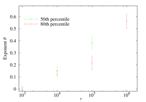
Recalling that time to solution is given by , we find that the exponent in Eq. (5) is less than 1 for all hardness groups, i.e., that the shorter the annealing time is, the shorter the time-to-solution becomes. Since however this trend can not hold all the way down to , these results therefore imply that there exist for each group an optimal annealing time that is however below the shortest-accessible s. Furthermore, the increase of with hardness group can be interpreted as the harder the instances are, the longer the typical optimal annealing time is, consistently with what one would expect from a quantum annealer. It is important to note at this point that the highly-fluctuating success probability, stemming from programming errors, unfortunately does note allow for a more sensitive analysis and that more robust results could be obtained if the programing errors leading to -chaos were to be reduced.
References
- Shor (1994) P. W. Shor, in Proc. 35th Symp. on Foundations of Computer Science, edited by S. Goldwasser (1994) p. 124.
- Grover (1997) L. K. Grover, Phys. Rev. Lett. 79, 325 (1997).
- Schlosshauer (2004) M. Schlosshauer, Rev. Mod. Phys. 76, 1267 (2004).
- Johnson et al. (2011) M. W. Johnson et al., Nature 473, 194 (2011).
- Albash et al. (2012) T. Albash, S. Boixo, D. A. Lidar, and P. Zanardi, New Journal of Physics 14, 123016 (2012).
- Lanting et al. (2014) T. Lanting, A. J. Przybysz, A. Y. Smirnov, F. M. Spedalieri, M. H. Amin, A. J. Berkley, R. Harris, F. Altomare, S. Boixo, P. Bunyk, N. Dickson, C. Enderud, J. P. Hilton, E. Hoskinson, M. W. Johnson, E. Ladizinsky, N. Ladizinsky, R. Neufeld, T. Oh, I. Perminov, C. Rich, M. C. Thom, E. Tolkacheva, S. Uchaikin, A. B. Wilson, and G. Rose, Phys. Rev. X 4, 021041 (2014).
- (7) J. A. Smolin and G. Smith, “Classical signature of quantum annealing,” ArXiv:1305.4904.
- Shin et al. (2014) S. W. Shin, G. Smith, J. A. Smolin, and U. Vazirani, arXiv:1401.7087 (2014).
- Ronnow et al. (2014) T. F. Ronnow, Z. Wang, J. Job, S. Boixo, S. V. Isakov, D. Wecker, J. M. Martinis, D. A. Lidar, and M. Troyer, Science 345, 420 (2014).
- Boixo et al. (2014) S. Boixo, T. F. Ronnow, S. V. Isakov, Z. Wang, D. Wecker, D. A. Lidar, J. M. Martinis, and M. Troyer, Nat Phys 10, 218 (2014).
- Young (1998) A. P. Young, ed., Spin Glasses and Random Fields (World Scientific, Singapore, 1998).
- Belletti et al. (2008) F. Belletti, M. Cotallo, A. Cruz, L. A. Fernandez, A. Gordillo, A. Maiorano, F. Mantovani, E. Marinari, V. Martin-Mayor, A. Muñoz Sudupe, D. Navarro, S. Perez-Gaviro, J. J. Ruiz-Lorenzo, S. F. Schifano, D. Sciretti, A. Tarancon, R. Tripiccione, and J. L. Velasco (Janus Collaboration), Comp. Phys. Comm. 178, 208 (2008), arXiv:0704.3573 .
- Belletti et al. (2009) F. Belletti, M. Guidetti, A. Maiorano, F. Mantovani, S. F. Schifano, R. Tripiccione, M. Cotallo, S. Perez-Gaviro, D. Sciretti, J. L. Velasco, A. Cruz, D. Navarro, A. Tarancon, L. A. Fernandez, V. Martin-Mayor, A. Muñoz-Sudupe, D. Yllanes, A. Gordillo-Guerrero, J. J. Ruiz-Lorenzo, E. Marinari, G. Parisi, M. Rossi, and G. Zanier (Janus Collaboration), Computing in Science and Engineering 11, 48 (2009).
- Baity-Jesi et al. (2014) M. Baity-Jesi, R. A. Baños, A. Cruz, L. A. Fernandez, J. M. Gil-Narvion, A. Gordillo-Guerrero, D. Iniguez, A. Maiorano, F. Mantovani, E. Marinari, V. Martin-Mayor, J. Monforte-Garcia, A. Muñoz Sudupe, D. Navarro, G. Parisi, S. Perez-Gaviro, M. Pivanti, F. Ricci-Tersenghi, J. J. Ruiz-Lorenzo, S. F. Schifano, B. Seoane, A. Tarancon, R. Tripiccione, and D. Yllanes (Janus Collaboration), Comp. Phys. Comm 185, 550 (2014), arXiv:1310.1032 .
- Hukushima and Nemoto (1996) K. Hukushima and K. Nemoto, J. Phys. Soc. Japan 65, 1604 (1996), arXiv:cond-mat/9512035 .
- Marinari (1998) E. Marinari, in Advances in Computer Simulation, edited by J. Kertész and I. Kondor (Springer-Verlag, 1998) p. 50, (arXiv:cond-mat/9612010).
- Kirkpatrick et al. (1983) S. Kirkpatrick, C. D. Gelatt, Jr., and M. P. Vecchi, Science 220, 671 (1983).
- Sokal (1997) A. Sokal, in Functional Integration: Basics and Applications, edited by C. DeWitt-Morette, P. Cartier, and A. Folacci (Plenum, 1997).
- Fernandez et al. (2009a) L. A. Fernandez, V. Martin-Mayor, S. Perez-Gaviro, A. Tarancon, and A. P. Young, Phys. Rev. B 80, 024422 (2009a).
- Alvarez Baños et al. (2010) R. Alvarez Baños, A. Cruz, L. A. Fernandez, J. M. Gil-Narvion, A. Gordillo-Guerrero, M. Guidetti, A. Maiorano, F. Mantovani, E. Marinari, V. Martin-Mayor, J. Monforte-Garcia, A. Muñoz Sudupe, D. Navarro, G. Parisi, S. Perez-Gaviro, J. J. Ruiz-Lorenzo, S. F. Schifano, B. Seoane, A. Tarancon, R. Tripiccione, and D. Yllanes (Janus Collaboration), J. Stat. Mech. 2010, P06026 (2010), arXiv:1003.2569 .
- Fernandez et al. (2013) L. A. Fernandez, V. Martin-Mayor, G. Parisi, and B. Seoane, EPL 103, 67003 (2013), arXiv:1307.2361 .
- McKay et al. (1982) S. R. McKay, A. N. Berker, and S. Kirkpatrick, Phys. Rev. Lett. 48, 767 (1982).
- Bray and Moore (1987) A. J. Bray and M. A. Moore, Phys. Rev. Lett. 58, 57 (1987).
- Banavar and Bray (1987) J. R. Banavar and A. J. Bray, Phys. Rev. B 35, 8888 (1987).
- Kondor (1989) I. Kondor, J. Phys. A 22, L163 (1989).
- Kondor and Végsö (1993) I. Kondor and Végsö, J. Phys. A 26, L641 (1993).
- Billoire and Marinari (2000) A. Billoire and E. Marinari, J. Phys. A 33, L265 (2000).
- Rizzo (2001) T. Rizzo, J. Phys. 34, 5531 (2001).
- Mulet et al. (2001) R. Mulet, A. Pagnani, and G. Parisi, Phys. Rev. B 63, 184438 (2001).
- Billoire and Marinari (2002) A. Billoire and E. Marinari, Europhys. Lett. 60, 775 (2002).
- Krzakala and Martin (2002) F. Krzakala and O. C. Martin, Eur. Phys. J. 28, 199 (2002).
- Rizzo and Crisanti (2003) T. Rizzo and A. Crisanti, Phys. Rev. Lett. 90, 137201 (2003).
- Parisi and Rizzo (2010) G. Parisi and T. Rizzo, J. Phys. A 43, 235003 (2010).
- Sasaki et al. (2005) M. Sasaki, K. Hukushima, H. Yoshino, and H. Takayama, Phys. Rev. Lett. 95, 267203 (2005).
- Katzgraber and Krzakala (2007) H. G. Katzgraber and F. Krzakala, Phys. Rev. Lett. 98, 017201 (2007).
- Billoire (2014) A. Billoire, J. Stat. Mech. 2014, P04016 (2014), arXiv:1401.4341 .
- Thomas et al. (2011) C. K. Thomas, D. A. Huse, and A. A. Middleton, Phys. Rev. Lett. 107, 047203 (2011), arXiv:1103.1946 .
- Katzgraber et al. (2014) H. G. Katzgraber, F. Hamze, and R. S. Andrist, Phys. Rev. X 4, 021008 (2014).
- Hamze and de Freitas (2004) F. Hamze and N. de Freitas, in Proceedings of the 20th Conference on Uncertainty in Artificial Intelligence, UAI ’04 (AUAI Press, Arlington, Virginia, United States, 2004) pp. 243–250.
- Selby (2014) A. Selby, “Efficient subgraph-based sampling of Ising-type models with frustration,” (2014), arXiv:1409.3934.
- Hen and Young (2011) I. Hen and A. P. Young, Phys. Rev. E. 84, 061152 (2011), arXiv:1109.6872v2 .
- Farhi et al. (2012) E. Farhi, D. Gosset, I. Hen, A. W. Sandvik, P. Shor, A. P. Young, and F. Zamponi, Phys. Rev. A 86, 052334 (2012), (arXiv:1208.3757 ).
- (43) Jamie King, Private Communication (2014).
- Cugliandolo et al. (1997) L. F. Cugliandolo, J. Kurchan, and L. Peliti, Phys. Rev. E 55, 3898 (1997).
- Nifle and Hilhorst (1992) M. Nifle and H. J. Hilhorst, Phys. Rev. Lett. 68, 2992 (1992).
- Ney-Nifle (1998) M. Ney-Nifle, Phys. Rev. B 57, 492 (1998).
- Krzakala and Bouchaud (2005) F. Krzakala and J. P. Bouchaud, Europhys. Lett. 72, 472 (2005).
- Pudenz et al. (2014) K. L. Pudenz, T. Albash, and D. A. Lidar, Nature Communications 5, 3243 (2014).
- Newman and Barkema (1999) M. E. J. Newman and G. T. Barkema, Monte Carlo Methods in Statistical Physics (Oxford University Press Inc., New York, USA, 1999).
- Fernandez et al. (2009b) L. A. Fernandez, V. Martin-Mayor, and D. Yllanes, Nucl. Phys. B 807, 424 (2009b).
- Barahona et al. (1982) F. Barahona, T. Maynard, R. Rammal, and J. P. Uhry, J. Phys. A 15, 673 (1982).
- Kadowaki and Nishimori (1998) T. Kadowaki and H. Nishimori, Phys. Rev. E 58, 5355 (1998).