Efficient batchwise dropout training using submatrices

Abstract

Dropout is a popular technique for regularizing artificial neural networks. Dropout networks are generally trained by minibatch gradient descent with a dropout mask turning off some of the units—a different pattern of dropout is applied to every sample in the minibatch. We explore a very simple alternative to the dropout mask. Instead of masking dropped out units by setting them to zero, we perform matrix multiplication using a submatrix of the weight matrix—unneeded hidden units are never calculated. Performing dropout batchwise, so that one pattern of dropout is used for each sample in a minibatch, we can substantially reduce training times. Batchwise dropout can be used with fully-connected and convolutional neural networks.

1 Independent versus batchwise dropout

Dropout is a technique to regularize artificial neural networks—it prevents overfitting [8]. A fully connected network with two hidden layers of 80 units each can learn to classify the MNIST training set perfectly in about 20 training epochs—unfortunately the test error is quite high, about 2%. Increasing the number of hidden units by a factor of 10 and using dropout results in a lower test error, about 1.1%. The dropout network takes longer to train in two senses: each training epoch takes several times longer, and the number of training epochs needed increases too. We consider a technique for speeding up training with dropout—it can substantially reduce the time needed per epoch.

Consider a very simple $\ell$-layer fully connected neural network with dropout. To train it with a minibatch of $b$ samples, the forward pass is described by the equations:

$$x_{k+1}=[x_{k}\cdot d_{k}]\times W_{k}\qquad k=0,\dots,\ell-1.$$

Here $x_{k}$ is a $b\times n_{k}$ matrix of input/hidden/output units, $d_{k}$ is a $b\times n_{k}$ dropout-mask matrix of independent Bernoulli($1-p_{k}$) random variables, $p_{k}$ denotes the probability of dropping out units in level $k$, and $W_{k}$ is an $n_{k}\times n_{k+1}$ matrix of weights connecting level $k$ with level $k+1$. We are using $\cdot$ for (Hadamard) element-wise multiplication and $\times$ for matrix multiplication. We have forgotten to include non-linear functions (e.g. the rectifier function for the hidden units, and softmax for the output units) but for the introduction we will keep the network as simple as possible.

The network can be trained using the backpropagation algorithm to calculate the gradients of a cost function (e.g. negative log-likelihood) with respect to the $W_{k}$:

$$\frac{\partial\mathrm{cost}}{\partial W_{k}} =[x_{k}\cdot d_{k}]^{\mathsf{T}}\times\frac{\partial\mathrm{cost}}{\partial x_{k+1}}$$

$$\frac{\partial\mathrm{cost}}{\partial x_{k}} =\left(\frac{\partial\mathrm{cost}}{\partial x_{k+1}}\times W_{k}^{\mathrm{\mathsf{T}}}\right)\cdot d_{k}.$$

With dropout training, we are trying to minimize the cost function averaged over an ensemble of closely related networks. However, networks typically contain thousands of hidden units, so the size of the ensemble is much larger than the number of training samples that can possibly be ‘seen’ during training. This suggests that the independence of the rows of the dropout mask matrices $d_{k}$ might not be terribly important; the success of dropout simply cannot depend on exploring a large fraction of the available dropout masks. Some machine learning libraries such as Pylearn2 allow dropout to be applied batchwise instead of independently. This is done by replacing $d_{k}$ with a $1\times n_{k}$ row matrix of independent Bernoulli$(1-p_{k})$ random variables, and then copying it vertically $b$ times to get the right shape.

To be practical, it is important that each training minibatch can be processed quickly. A crude way of estimating the processing time is to count the number of floating point multiplication operations needed (naively) to evaluate the $\times$ matrix multiplications specified above:

$$\sum_{k=0}^{\ell-1}\underbrace{b\times n_{k}\times n_{k+1}}_{\mathrm{forwards}}+\underbrace{n_{k}\times b\times n_{k+1}}_{\partial\mathrm{cost/\partial}W}+\underbrace{b\times n_{k+1}\times n_{k}}_{\mathrm{backwards}}.$$

However, when we take into account the effect of the dropout mask, we see that many of these multiplications are unnecessary. The $(i,j)$-th element of the $W_{k}$ weight matrix effectively ‘drops-out’ of the calculations if unit $i$ is dropped in level $k$, or if unit $j$ is dropped in level $k+1$. Applying 50% dropout in levels $k$ and $k+1$ renders 75% of the multiplications unnecessary.

If we apply dropout independently, then the parts of $W_{k}$ that disappear are different for each sample. This makes it effectively impossible to take advantage of the redundancy—it is slower to check if a multiplication is necessary than to just do the multiplication. However, if we apply dropout batchwise, then it becomes easy to take advantage of the redundancy. We can literally drop-out redundant parts of the calculations.

The binary $1\times n_{k}$ batchwise dropout matrices $d_{k}$ naturally define submatrices of the weight and hidden-unit matrices. Let $x_{k}^{\mathrm{dropout}}:=x_{k}[\,:\,,d_{k}]$ denote the submatrix of $x_{k}$ consisting of the level-$k$ hidden units that survive dropout. Let $W_{k}^{\mathrm{dropout}}:=W_{k}[d_{k},d_{k+1}]$ denote the submatrix of $W_{k}$ consisting of weights that connect active units in level $k$ to active units in level $k+1$. The network can then be trained using the equations:

$$x_{k+1}^{\mathrm{dropout}} =x_{k}^{\mathrm{dropout}}\times W_{k}^{\mathrm{dropout}}$$

$$\frac{\partial\mathrm{cost}}{\partial W_{k}^{\mathrm{dropout}}} =(x_{k}^{\mathrm{dropout}})^{\mathsf{T}}\times\frac{\partial\mathrm{cost}}{\partial x_{k+1}^{\mathrm{dropout}}}$$

$$\frac{\partial\mathrm{cost}}{\partial x_{k}^{\mathrm{dropout}}} =\frac{\partial\mathrm{cost}}{\partial x_{k+1}^{\mathrm{dropout}}}\times(W_{k}^{\mathrm{dropout}})^{\mathsf{T}}$$

The redundant multiplications have been eliminated. There is an additional benefit in terms of memory needed to store the hidden units: $x_{k}^{\mathrm{dropout}}$ needs less space than $x_{k}$. In Section 2 we look at the performance improvement that can be achieved using CUDA/CUBLAS code running on a GPU. Roughly speaking, processing a minibatch with 50% batchwise dropout takes as long as training a 50% smaller network on the same data. This explains the nearly overlapping pairs of lines in Figure 1.

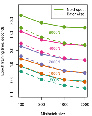
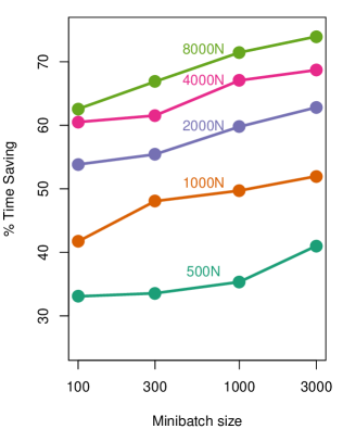
Figure 1: Left: MNIST training time for three layer networks (log scales) on an NVIDIA GeForce GTX 780 graphics card. Right: Percentage reduction in training times moving from no dropout to batchwise dropout. The time saving for the 500N network with minibatches of size 100 increases from 33% to 42% if you instead compare batchwise dropout with independent dropout.

We should emphasize that batchwise dropout only improves performance during training; during testing the full $W_{k}$ matrix is used as normal, scaled by a factor of $1-p_{k}$. However, machine learning research is often constrained by long training times and high costs of equipment. In Section 3 we show that all other things being equal, batchwise dropout is similar to independent dropout, but faster. Moreover, with the increase in speed, all other things do not have to be equal. With the same resources, batchwise dropout can be used to

• increase the number of training epochs,

• increase the number of hidden units,

• increase the number of validation runs used to optimize “hyper-parameters”, or

• to train a number of independent copies of the network to form a committee.

These possibilities will often be useful as ways of improving generalization/reducing test error.

In Section 4 we look at batchwise dropout for convolutional networks. Dropout for convolutional networks is more complicated as weights are shared across spatial locations. A minibatch passing up through a convolutional network might be represented at an intermediate hidden layer by an array of size $100\times 32\times 12\times 12$: 100 samples, the output of 32 convolutional filters, at each of $12\times 12$ spatial locations. It is conventional to use a dropout mask with shape $100\times 32\times 12\times 12$; we will call this independent dropout. In contrast, if we want to apply batchwise dropout efficiently by adapting the submatrix trick, then we will effectively be using a dropout mask with shape $1\times 32\times 1\times 1$. This looks like a significant change: we are modifying the ensemble over which the average cost is optimized. During training, the error rates are higher. However, testing the networks gives very similar error rates.

1.1 Fast dropout

We might have called batchwise dropout fast dropout but that name is already taken [11]. Fast dropout is very different approach to solving the problem of training large neural network quickly without overfitting. We discuss some of the differences of the two techniques in the appendix.

2 Implementation

In theory, for $n\times n$ matrices, addition is an $\mathrm{O}(n^{2})$ operation, and multiplication is $\mathrm{O}(n^{2.37...})$ by the Coppersmith–Winograd algorithm. This suggests that the bulk of our processing time should be spent doing matrix multiplication, and that a performance improvement of about 60% should be possible compared to networks using independent dropout, or no dropout at all. In practice, SGEMM functions use Strassen’s algorithm or naive matrix multiplication, so performance improvement of up to 75% should be possible.

We implemented batchwise dropout for fully-connected and convolutional neural networks using CUDA/CUBLAS. We found that using the highly optimized cublasSgemm function to do the bulk of the work, with CUDA kernels used to form the submatrices $W_{k}^{\mathrm{dropout}}$ and to update the $W_{k}$ using $\partial\mathrm{cost}/\partial W_{k}^{\mathrm{dropout}}$, worked well. Better performance may well be obtained by writing a SGEMM-like matrix multiplication function that understands submatrices.

For large networks and minibatches, we found that batchwise dropout was substantially faster, see Figure 1. The approximate overlap of some of the lines on the left indicates that 50% batchwise dropout reduces the training time in a similar manner to halving the number of hidden units.

The graph on the right show the time saving obtained by using submatrices to implement dropout. Note that for consistency with the left hand side, the graph compares batchwise dropout with dropout-free networks, not with networks using independent dropout. The need to implement dropout masks for independent dropout means that Figure 1 slightly undersells the performance benefits of batchwise dropout as an alternative to independent dropout.

For smaller networks, the performance improvement is lower—bandwidth issues result in the GPU being under utilized. If you were implementing batchwise dropout for CPUs, you would expect to see greater performance gains for smaller networks as CPUs have a lower processing-power to bandwidth ratio.

2.1 Efficiency tweaks

If you have $n=2000$ hidden units and you drop out $p=50$% of them, then the number of dropped units is approximately $np=1000$, but with some small variation as you are really dealing with a Binomial$(n,p)$ random variable—its standard deviation is $\sqrt{np(1-p)}=22.4$. The sizes of the submatrices $W_{k}^{\mathrm{dropout}}$ and $x_{k}^{\mathrm{dropout}}$ are therefore slightly random. In the interests of efficiency and simplicity, it is convenient to remove this randomness. An alternative to dropping each unit independently with probability $p$ is to drop a subset of exactly $np$ of the hidden units, uniformly at random from the set of all $\binom{n}{np}$ such subsets. It is still the case that each unit is dropped out with probability $p$. However, within a hidden layer we no longer have strict independence regarding which units are dropped out. The probability of dropping out the first two hidden units changes very slightly, from

$$p^{2}=0.25\qquad\mathrm{to}\qquad\frac{np}{n}\cdot\frac{np-1}{n-1}=0.24987....$$

Also, we used a modified form of NAG-momentum minibatch gradient descent [9]. After each minibatch, we only updated the elements of $W_{k}^{\mathrm{dropout}}$, not all the element of $W_{k}$. With $v_{k}$ and $v_{k}^{\mathrm{dropout}}$ denoting the momentum matrix/submatrix corresponding to $W_{k}$ and $W_{k}^{\mathrm{dropout}}$, our update was

$$v_{k}^{\mathrm{dropout}} \leftarrow\mu v_{k}^{\mathrm{dropout}}-\varepsilon(1-\mu)\partial\mathrm{cost}/\partial W_{k}^{\mathrm{dropout}}$$

$$W_{k}^{\mathrm{dropout}} \leftarrow W_{k}^{\mathrm{dropout}}+v_{k}^{\mathrm{dropout}}.$$

The momentum still functions as an autoregressive process, smoothing out the gradients, we are just reducing the rate of decay $\mu$ by a factor of $(1-p_{k})(1-p_{k+1})$.

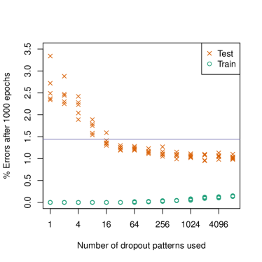
Figure 2: Dropout networks trained using a restricted the number of dropout patterns (each $\times$ is from an independent experiment). The blue line marks the test error for a network with half as many hidden units trained without dropout.

3 Results for fully-connected networks

The fact that batchwise dropout takes less time per training epoch would count for nothing if a much larger number of epochs was needed to train the network, or if a large number of validation runs were needed to optimize the training process. We have carried out a number of simple experiment to compare independent and batchwise dropout. In many cases we could have produced better results by increasing the training time, annealing the learning rate, using validation to adjust the learning process, etc. We choose not to do this as the primary motivation for batchwise dropout is efficiency, and excessive use of fine-tuning is not efficient.

For datasets, we used:

• The MNIST set of $28\times 28$ pixel handwritten digits.

• The CIFAR-10 dataset of 32x32 pixel color pictures ([4]).

• An artificial dataset designed to be easy to overfit.

Following [8], for MNIST and CIFAR-10 we trained networks with 20% dropout in the input layer, and 50% dropout in the hidden layers. For the artificial dataset we increased the input-layer dropout to 50% as this reduced the test error. In some cases, we have used relatively small networks so that we would have time to train a number of independent copies of the networks. This was useful in order to see if the apparent differences between batchwise and independent dropout are significant or just noise.

3.1 MNIST

Our first experiment explores the effect of dramatically restricting the number of dropout patterns seen during training. Consider a network with three hidden layers of size 1000, trained for 1000 epochs using minibatches of size 100. The number of distinct dropout patterns, $2^{3784}$, is so large that we can assume that we will never generate the same dropout mask twice. During independent dropout training we will see 60 million different dropout patterns, during batchwise dropout training we will see 100 times fewer dropout patterns.

For both types of dropout, we trained 12 independent networks for 1000 epochs, with batches of size 100. For batchwise dropout we got a mean test error of 1.04% [range (0.92%,1.1%), s.d. 0.057%] and for independent dropout we got a mean test errors of 1.03% [range (0.98%,1.08%), s.d. 0.033%]. The difference in the mean test errors is not statistically significant.

To explore further the reduction in the number of dropout patterns seen, we changed our code for (pseudo)randomly generating batchwise dropout patterns to restrict the number of distinct dropout patterns used. We modified it to have period $n$ minibatches, with $n=1,2,4,8,\dots$; see Figure 2. For $n=1$ this corresponds to only ever using one dropout mask, so that 50% of the network’s 3000 hidden weights are never actually trained (and 20% of the 784 input features are ignored). During training this corresponds to training a dropout-free network with half as many hidden units—the test error for such a network is marked by a blue line in Figure 2. The error during testing is higher than the blue line because the untrained weights add noise to the network.

If $n$ is less than thirteen, is it likely that some of the networks 3000 hidden units are dropped out every time and so receive no training. If $n$ is in the range thirteen to fifty, then it is likely that every hidden unit receives some training, but some pairs of hidden units in adjacent layers will not get the chance to interact during training, so the corresponding connection weight is untrained. As the number of dropout masks increases into the hundreds, we see that it is quickly a case of diminishing returns.

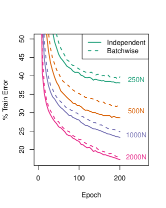
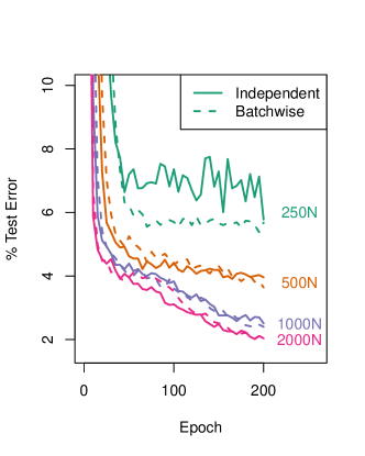
Figure 3: Artificial dataset. 100 classes each corresponding to noisy observations of a one dimensional manifold in $\{0,1\}^{1000}$.

3.2 Artificial dataset

To test the effect of changing network size, we created an artificial dataset. It has 100 classes, each containing 1000 training samples and 100 test samples. Each class is defined using an independent random walk of length 1000 in the discrete cube $\{0,1\}^{1000}$. For each class we generated the random walk, and then used it to produce the training and test samples by randomly picking points along the length of walk (giving binary sequences of length 1000) and then randomly flipping 40% of the bits. We trained three layer networks with $n\in\{250,500,1000,2000\}$ hidden units per layer with minibatches of size 100. See Figure 3.

Looking at the training error against training epochs, independent dropout seems to learn slightly faster. However, looking at the test errors over time, there does not seem to be much difference between the two forms of dropout. Note that the $x$-axis is the number of training epochs, not the training time. The batchwise dropout networks are learning much faster in terms of real time.

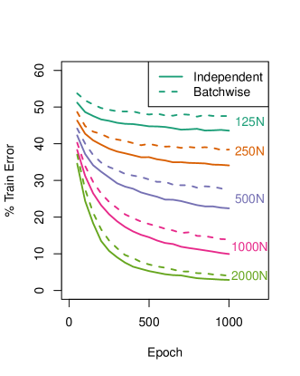
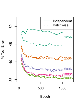
Figure 4: Results for CIFAR-10 using fully-connected networks of different sizes.

3.3 CIFAR-10 fully-connected

Learning CIFAR-10 using a fully connected network is rather difficult. We trained three layer networks with $n\in\{125,250,500,1000,2000\}$ hidden units per layer with minibatches of size 1000. We augmented the training data with horizontal flips. See Figure 4.

4 Convolutional networks

Dropout for convolutional networks is more complicated as weights are shared across spatial locations. Suppose layer $k$ has spatial size $s_{k}\times s_{k}$ with $n_{k}$ features per spatial location, and if the $k$-th operation is a convolution with $f\times f$ filters. For a minibatch of size $b$, the convolution involves arrays with sizes:

$$\mathrm{layer}\ k: \ b\times n_{k}\times s_{k}\times s_{k}$$

$$\mathrm{weights\ }W_{k}: \ n_{k+1}\times n_{k}\times f\times f$$

Dropout is normally applied using dropout masks with the same size as the layers. We will call this independent dropout—independent decisions are mode at every spatial location. In contrast, we define batchwise dropout to mean using a dropout mask with shape $1\times n_{k}\times 1\times 1$. Each minibatch, each convolutional filter is either on or off—across all spatial locations.

These two forms of regularization seem to be doing quite different things. Consider a filter that detects the color red, and a picture with a red truck in it. If dropout is applied independently, then by the law of averages the message “red” will be transmitted with very high probability, but with some loss of spatial information. In contrast, with batchwise dropout there is a 50% chance we delete the entire filter output. Experimentally, the only substantial difference we could detect was that batchwise dropout resulted in larger errors during training.

To implement batchwise dropout efficiently, notice that the $1\times n_{k}\times 1\times 1$ dropout masks corresponds to forming subarrays $W_{k}^{\mathrm{dropout}}$ of the weight arrays $W_{k}$ with size

$$(1-p_{k+1})n_{k+1}\times(1-p_{k})n_{k}\times f\times f.$$

The forward-pass is then simply a regular convolutional operation using $W_{k}^{\mathrm{dropout}}$; that makes it possible, for example, to take advantage of the highly optimized $\mathsf{cudnnConvolutionForward}$ function from the NVIDIA cuDNN package.

4.1 MNIST

For MNIST, we trained a LeNet-5 type CNN with two layers of $5\times 5$ filters, two layers of $2\times 2$ max-pooling, and a fully connected layer [6]. There are three places for applying 50% dropout:

$$32\mathrm{C}5-\mathrm{MP2}\overset{50\%}{-}64\mathrm{C}5-\mathrm{MP2}\overset{50\%}{-}512\mathrm{N}\overset{50\%}{-}\mathrm{10N}.$$

The test errors for the two dropout methods are similar, see Figure 5.

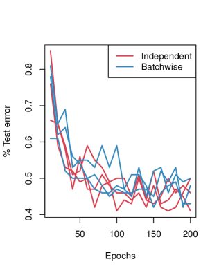
Figure 5: MNIST test errors, training repeated three times for both dropout methods.

4.2 CIFAR-10 with varying dropout intensity

For a first experiment with CIFAR-10 we used a small convolutional network with small filters. The network is a scaled down version of the network from [1]; there are four places to apply dropout:

$$128\mathrm{C}3-\mathrm{MP2}\overset{p}{-}256\mathrm{C2}-\mathrm{MP2}\overset{p}{-}384\mathrm{C2}-\mathrm{MP2}\overset{p}{-}512\mathrm{N}\overset{p}{-}\mathrm{10N}.$$

The input layer is $24\times 24$. We trained the network for 1000 epochs using randomly chosen subsets of the training images, and reflected each image horizontally with probability one half. For testing we used the centers of the images.

In Figure 6 we show the effect of varying the dropout probability $p$. The training errors are increasing with $p$, and the training errors are higher for batchwise dropout. The test-error curves both seem to have local minima around $p=0.2$. The batchwise test error curve seems to be shifted slightly to the left of the independent one, suggesting that for any given value of $p$, batchwise dropout is a slightly stronger form of regularization.

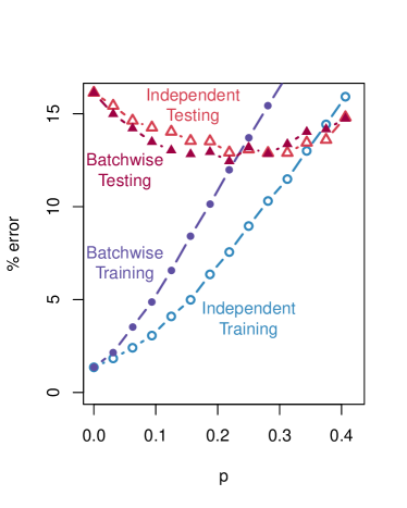
Figure 6: CIFAR-10 results using a convolutional network with dropout probability $p\in(0,0.4)$. Batchwise dropout produces a slightly lower minimum test error.

4.3 CIFAR-10 with many convolutional layers

We trained a deep convolutional network on CIFAR-10 without data augmentation. Using the notation of [2], our network has the form

$$(64nC2-FMP\sqrt[3]{2})_{12}-832C2-896C1-\mathrm{output},$$

i.e. it consists of 12 $2\times 2$ convolutions with $64n$ filters in the $n$-th layer, 12 layers max-pooling, followed by two fully connected layers; the network has 12.6 million parameters. We used an increasing amount of dropout per layer, rising linearly from 0% dropout after the third layer to 50% dropout after the 14th. Even though the amount of dropout used in the middle layers is small, batchwise dropout took less than half as long per epoch as independent dropout; this is because applying small amounts of independent dropout in large hidden-layers creates a bandwidth performance-bottleneck.

As the network’s max-pooling operation is stochastic, the test errors can be reduced by repetition. Batchwise dropout resulted in a average test error of 7.70% (down to 5.78% with 12-fold testing). Independent dropout resulted in an average test error of 7.63% (reduced to 5.67% with 12-fold testing).

5 Conclusions and future work

We have implemented an efficient form of batchwise dropout. All other things being equal, it seems to learn at roughly the same speed as independent dropout, but each epoch is faster. Given a fixed computational budget, it will often allow you to train better networks.

There are other potential uses for batchwise dropout that we have not explored yet:

• Restricted Boltzmann Machines can be trained by contrastive divergence [3] with dropout [8]. Batchwise dropout could be used to increase the speed of training.

• When a fully connected network sits on top of a convolutional network, training the top and bottom of the network can be separated over different computational nodes [5]. The fully connected top-parts of the network typically contains 95% of the parameters—keeping the nodes synchronized is difficult due to the large size of the matrices. With batchwise dropout, nodes could communicate $\partial\mathrm{cost}/\partial W_{k}^{\mathrm{dropout}}$ instead of $\partial\mathrm{cost}/\partial W_{k}$ and so reducing the bandwidth needed.

• Using independent dropout with recurrent neural networks can be too disruptive to allow effective learning; one solution is to only apply dropout to some parts of the network [12]. Batchwise dropout may provide a less damaging form of dropout, as each unit will either be on or off for the whole time period.

• Dropout is normally only used during training. It is generally more accurate use the whole network for testing purposes; this is equivalent to averaging over the ensemble of dropout patterns. However, in a “real-time” setting, such as analyzing successive frames from a video camera, it may be more efficient to use dropout during testing, and then to average the output of the network over time.

• Nested dropout [7] is a variant of regular dropout that extends some of the properties of PCA to deep networks. Batchwise nested dropout is particularly easy to implement as the submatrices are regular enough to qualify as matrices in the context of the SGEMM function (using the LDA argument).

• DropConnect is an alternative form of regularization to dropout [10]. Instead of dropping hidden units, individual elements of the weight matrix are dropped out. Using a modification similar to the one in Section 2.1, there are opportunities for speeding up DropConnect training by approximately a factor of two.

Appendix A Fast dropout

We might have called batchwise dropout fast dropout but that name is already taken [11]. Fast dropout is an alternative form of regularization that uses a probabilistic modeling technique to imitate the effect of dropout; each hidden unit is replaced with a Gaussian probability distribution. The fast relates to reducing the number of training epochs needed compared to regular dropout (with reference to results in a preprint of [8]). Training a network 784-800-800-10 on the MNIST dataset with 20% input dropout and 50% hidden-layer dropout, fast dropout converges to a test error of 1.29% after 100 epochs of L-BFGS. This appears to be substantially better than the test error obtained in the preprint after 100 epochs of regular dropout training.

However, this is a dangerous comparison to make. The authors of [8] used a learning-rate scheme designed to produce optimal accuracy eventually, not after just one hundred epochs. We tried using batchwise dropout with minibatches of size 100 and an annealed learning rate of $0.01e^{-0.01\times\mathrm{epoch}}$. We trained a network with two hidden layers of 800 rectified linear units each. Training for 100 epochs resulted in a test error of 1.22% (s.d. 0.03%). After 200 epochs the test error has reduced further to 1.12% (s.d. 0.04%). Moreover, per epoch, batchwise-dropout is faster than regular dropout while fast-dropout is slower. Assuming we can make comparisons across different programs, the 200 epochs of batchwise dropout training take less time than the 100 epoch of fast dropout training.

References

- [1] D. Ciresan, U. Meier, and J. Schmidhuber. Multi-column deep neural networks for image classification. In Computer Vision and Pattern Recognition (CVPR), 2012 IEEE Conference on, pages 3642–3649, 2012.
- [2] Ben Graham. Fractional max-pooling, 2014. http://arxiv.org/abs/1412.6071.
- [3] Hinton and Salakhutdinov. Reducing the Dimensionality of Data with Neural Networks. SCIENCE: Science, 313, 2006.
- [4] Alex Krizhevsky. Learning Multiple Layers of Features from Tiny Images. Technical report, 2009.
- [5] Alex Krizhevsky. One weird trick for parallelizing convolutional neural networks, 2014. http://arxiv.org/abs/1404.5997.
- [6] Y. L. Le Cun, L. Bottou, Y. Bengio, and P. Haffner. Gradient-based learning applied to document recognition. Proceedings of IEEE, 86(11):2278–2324, November 1998.
- [7] Oren Rippel, Michael A. Gelbart, and Ryan P. Adams. Learning ordered representations with nested dropout, 2014. http://arxiv.org/abs/1402.0915.
- [8] Nitish Srivastava, Geoffrey Hinton, Alex Krizhevsky, Ilya Sutskever, and Ruslan Salakhutdinov. Dropout: A Simple Way to Prevent Neural Networks from Overfitting. Journal of Machine Learning Research, 15:1929–1958, 2014.
- [9] Ilya Sutskever, James Martens, George E. Dahl, and Geoffrey E. Hinton. On the importance of initialization and momentum in deep learning. In ICML, volume 28 of JMLR Proceedings, pages 1139–1147. JMLR.org, 2013.
- [10] Li Wan, Matthew Zeiler, Sixin Zhang, Yann Lecun, and Rob Fergus. Regularization of Neural Networks using DropConnect, 2013. JMLR W&CP 28 (3) : 1058–1066, 2013.
- [11] Sida Wang and Christopher Manning. Fast dropout training. JMLR W & CP, 28(2):118–126, 2013.
- [12] Wojciech Zaremba, Ilya Sutskever, and Oriol Vinyals. Recurrent neural network regularization, 2014. http://arxiv.org/abs/1409.2329.