Structural Decompositions for Problems
with Global Constraints

Abstract

A wide range of problems can be modelled as constraint satisfaction problems (CSPs), that is, a set of constraints that must be satisfied simultaneously. Constraints can either be represented extensionally, by explicitly listing allowed combinations of values, or implicitly, by special-purpose algorithms provided by a solver.

Such implicitly represented constraints, known as global constraints, are widely used; indeed, they are one of the key reasons for the success of constraint programming in solving real-world problems. In recent years, a variety of restrictions on the structure of CSP instances have been shown to yield tractable classes of CSPs. However, most such restrictions fail to guarantee tractability for CSPs with global constraints. We therefore study the applicability of structural restrictions to instances with such constraints.

We show that when the number of solutions to a CSP instance is bounded in key parts of the problem, structural restrictions can be used to derive new tractable classes. Furthermore, we show that this result extends to combinations of instances drawn from known tractable classes, as well as to CSP instances where constraints assign costs to satisfying assignments.

1 Introduction

Constraint programming (CP) is widely used to solve a variety of practical problems such as planning and scheduling vanHoeve2006:global-const ; Wallace96practicalapplications , and industrial configuration pup-cpaior2011 ; bin-repack-datacenters . Constraints can either be represented explicitly, by a table of allowed assignments, or implicitly, by specialized algorithms provided by the constraint solver. These algorithms may take as a parameter a description that specifies exactly which kinds of assignments a particular instance of a constraint should allow. Such implicitly represented constraints are known as global constraints, and a lot of the success of CP in practice has been attributed to solvers providing global constraints Rossi06:handbook ; Gent06:minion ; wallace97-eclipse .

The theoretical properties of constraint problems, in particular the computational complexity of different types of problem, have been extensively studied and quite a lot is known about what restrictions on the general constraint satisfaction problem are sufficient to make it tractable struct-decomp-stacs-et ; bulatov05:classifying-constraints ; CohenUnifTract ; compar-decomp-csp ; grohe-hom-csp-complexity ; DBLP:journals/corr/abs-0911-0801 . In particular, many structural restrictions, that is, restrictions on how the constraints in a problem interact, have been identified and shown to yield tractable classes of CSP instances Gottlob02:jcss-hypertree ; grohe-marx-frac-edge-cover ; DBLP:journals/corr/abs-0911-0801 . However, much of this theoretical work has focused on problems where each constraint is explicitly represented, and most known structural restrictions fail to yield tractable classes for problems with global constraints. This is the case even when the global constraints are fairly simple, such as overlapping difference constraints with acyclic hypergraphs Kutz08:sim-match .

Theoretical work on global constraints has to a large extent focused on developing efficient algorithms to achieve various kinds of local consistency for individual constraints. This is generally done by pruning from the domains of variables those values that cannot lead to a satisfying assignment Walsh07:global ; Samer11:constraints-tractable . Another strand of research has explored conditions that allow global constraints to be replaced by collections of explicitly represented constraints bess-nvalue . These techniques allow faster implementations of algorithms for individual constraints, but do not shed much light on the complexity of problems with multiple overlapping global constraints, which is something that practical problems frequently require.

As such, in this paper we investigate the properties of explicitly represented constraints that allow structural restrictions to guarantee tractability. Identifying such properties will allow us to find global constraints that also possess them, and lift structural restrictions to instances with such constraints.

As discussed in ChenGroheCompactRel , when the constraints in a family of problems have unbounded arity, the way that the constraints are represented can significantly affect the complexity. Previous work in this area has assumed that the global constraints have specific representations, such as propagators Green08:cp-structural , negative constraints gdnf-cohen-repr , or GDNF/decision diagrams ChenGroheCompactRel , and exploited properties particular to that representation. In contrast, we will use a definition of global constraints, used also in cp-tract-comb , that allows us to discuss different representations in a uniform manner. Armed with this definition, we obtain results that rely on a relationship between the size of a global constraint and the number of its satisfying assignments.

Furthermore, as our definition is general enough to capture arbitrary problems in , we demonstrate how our results can be used to decompose a constraint problem into smaller constraint problems (as opposed to individual constraints), and when such decompositions lead to tractability. The results that we obtain on this topic extend previous research by Cohen and Green guarded-decomp-CG . In addition to being more general, our results arguably use simpler theoretical machinery.

Finally, we show how our results can be extended to weighted CSP gottlob-etal-tractable-optimization ; degivry06 , that is, CSP where constraints assign costs to satisfying assignments, and the goal is to find an optimal solution.

2 Preliminaries

In this section, we define the basic concepts that we will use throughout the paper. In particular, we give a precise definition of global constraints and of structural decompositions.

2.1 Global Constraints

Definition 1 (Variables and assignments).

Let $V$ be a set of variables, each with an associated finite set of domain elements. We denote the set of domain elements (the domain) of a variable $v$ by $D(v)$. We extend this notation to arbitrary subsets of variables, $W$, by setting $D(W)=\displaystyle\bigcup_{v\in W}D(v)$.

An assignment of a set of variables $V$ is a function $\theta:V\rightarrow D(V)$ that maps every $v\in V$ to an element $\theta(v)\in D(v)$. We write $\mathcal{V}(\theta)$ for the set of variables $V$.

We denote the restriction of $\theta$ to a set of variables $W\subseteq V$ by $\theta|_{W}$. We also allow the special assignment $\bot$ of the empty set of variables. In particular, for every assignment $\theta$, we have $\theta|_{\emptyset}=\bot$.

Definition 2 (Projection).

Let $\Theta$ be a set of assignments of a set of variables $V$. The projection of $\Theta$ onto a set of variables $X\subseteq V$ is the set of assignments $\pi_{X}(\Theta)=\{\theta|_{X}\mid\theta\in\Theta\}$.

Note that when $\Theta=\emptyset$ we have $\pi_{X}(\Theta)=\emptyset$, but when $X=\emptyset$ and $\Theta\neq\emptyset$, we have $\pi_{X}(\Theta)=\{\bot\}$.

Definition 3 (Disjoint union of assignments).

Let $\theta_{1}$ and $\theta_{2}$ be two assignments of disjoint sets of variables $V_{1}$ and $V_{2}$, respectively. The disjoint union of $\theta_{1}$ and $\theta_{2}$, denoted $\theta_{1}\oplus\theta_{2}$, is the assignment of $V_{1}\cup V_{2}$ such that $(\theta_{1}\oplus\theta_{2})(v)=\theta_{1}(v)$ for all $v\in V_{1}$, and $(\theta_{1}\oplus\theta_{2})(v)=\theta_{2}(v)$ for all $v\in V_{2}$.

Global constraints have traditionally been defined, somewhat vaguely, as constraints without a fixed arity, possibly also with a compact representation of the constraint relation. For example, in vanHoeve2006:global-const a global constraint is defined as “a constraint that captures a relation between a non-fixed number of variables”.

Below, we offer a precise definition similar to the one in Walsh07:global , where the authors define global constraints for a domain $D$ over a list of variables $\sigma$ as being given intensionally by a function $D^{|\sigma|}\rightarrow\{0,1\}$ computable in polynomial time. Our definition differs from this one in that we separate the general algorithm of a global constraint (which we call its type) from the specific description. This separation allows us a better way of measuring the size of a global constraint, which in turn helps us to establish new complexity results.

Definition 4 (Global constraints).

A global constraint type is a parameterized polynomial-time algorithm that determines the acceptability of an assignment of a given set of variables.

Each global constraint type, $e$, has an associated set of descriptions, $\Delta(e)$. Each description $\delta\in\Delta(e)$ specifies appropriate parameter values for the algorithm $e$. In particular, each $\delta\in\Delta(e)$ specifies a set of variables, denoted by $\mathcal{V}(\delta)$. We write $|\delta|$ for the number of bits used to represent $\delta$.

A global constraint $e[\delta]$, where $\delta\in\Delta(e)$, is a function that maps assignments of $\mathcal{V}(\delta)$ to the set $\{0,1\}$. Each assignment that is allowed by $e[\delta]$ is mapped to 1, and each disallowed assignment is mapped to 0. The extension or constraint relation of $e[\delta]$ is the set of assignments, $\theta$, of $\mathcal{V}(\delta)$ such that $e[\delta](\theta)=1$. We also say that such assignments satisfy the constraint, while all other assignments falsify it.

When we are only interested in describing the set of assignments that satisfy a constraint, and not in the complexity of determining membership in this set, we will sometimes abuse notation by writing $\theta\in e[\delta]$ to mean $e[\delta](\theta)=1$.

As can be seen from the definition above, a global constraint is not usually explicitly represented by listing all the assignments that satisfy it. Instead, it is represented by some description $\delta$ and some algorithm $e$ that allows us to check whether the constraint relation of $e[\delta]$ includes a given assignment. To stay within the complexity class , this algorithm is required to run in polynomial time. As the algorithms for many kinds of global constraints are built into modern constraint solvers, we measure the size of a global constraint’s representation by the size of its description.

Example 1 (EGC).

A very general global constraint type is the extended global cardinality constraint type Samer11:constraints-tractable . This form of global constraint is defined by specifying, for every domain element $a$, a finite set of natural numbers $K(a)$, called the cardinality set of $a$. The constraint requires that the number of variables which are assigned the value $a$ is in the set $K(a)$, for each possible domain element $a$.

Using our notation, the description $\delta$ of an EGC global constraint specifies a function $K_{\delta}:D(\mathcal{V}(\delta))\rightarrow\mathcal{P}(\mathbb{N})$ that maps each domain element to a set of natural numbers. The algorithm for the EGC constraint then maps an assignment $\theta$ to $1$ if and only if, for every domain element $a\in D(\mathcal{V}(\delta))$, we have that $|\{v\in\mathcal{V}(\delta)\mid\theta(v)=a\}|\in K_{\delta}(a)$.

Example 2 (Table and negative constraints).

A rather degenerate example of a a global constraint type is the table constraint.

In this case the description $\delta$ is simply a list of assignments of some fixed set of variables, $\mathcal{V}(\delta)$. The algorithm for a table constraint then decides, for any assignment of $\mathcal{V}(\delta)$, whether it is included in $\delta$. This can be done in a time which is linear in the size of $\delta$ and so meets the polynomial time requirement.

Negative constraints are complementary to table constraints, in that they are described by listing forbidden assignments. The algorithm for a negative constraint $e[\delta]$ decides, for any assignment of $\mathcal{V}(\delta)$, whether it is not included in $\delta$. Observe that disjunctive clauses, used to define propositional satisfiability problems, are a special case of the negative constraint type, as they have exactly one forbidden assignment.

We observe that any global constraint can be rewritten as a table or negative constraint. However, this rewriting will, in general, incur an exponential increase in the size of the description.

As can be seen from the definition above, a table global constraint is explicitly represented, and thus equivalent to the usual notion of an extensionally represented constraint.

In some cases, particularly for table constraints, we will make use of the standard notion of a relational join, which we define below.

Definition 5 (Constraint join).

A global constraint $e_{j}[\delta_{j}]$ is the join of two global constraints $e_{1}[\delta_{1}]$ and $e_{2}[\delta_{2}]$ whenever $\mathcal{V}(\delta_{j})=\mathcal{V}(\delta_{1})\cup\mathcal{V}(\delta_{2})$, and $\theta\in e_{j}[\delta_{j}]$ if and only if $\theta|_{\mathcal{V}(\delta_{1})}\in e_{1}[\delta_{1}]$ and $\theta|_{\mathcal{V}(\delta_{2})}\in e_{2}[\delta_{2}]$.

Definition 6 (CSP instance).

An instance of the constraint satisfaction problem (CSP) is a pair $\langle V,C\rangle$ where $V$ is a finite set of variables, and $C$ is a set of global constraints such that $V=\displaystyle\bigcup_{e[\delta]\in C}\mathcal{V}(\delta)$. In a CSP instance, we call $\mathcal{V}(\delta)$ the scope of the constraint $e[\delta]$.

A classic CSP instance is one where every constraint is a table constraint.

A solution to a CSP instance $P=\langle V,C\rangle$ is an assignment $\theta$ of $V$ which satisfies every global constraint, i.e., for every $e[\delta]\in C$ we have $\theta|_{\mathcal{V}(\delta)}\in e[\delta]$. We denote the set of solutions to $P$ by $\mathsf{sol}(P)$.

The size of a CSP instance $P=\langle V,C\rangle$ is $|P|=|V|+\displaystyle\sum_{v\in V}|D(v)|+\displaystyle\sum_{e[\delta]\in C}|\delta|$.

Note that this definition disallows CSP instances with variables that are not in the scope of any constraint. Since a variable that is not in the scope of any constraint can be assigned any value from its domain, excluding such variables can be done without loss of generality. While this condition is strictly speaking not necessary, it will allow us to simplify some proofs later on. In particular, it entails that the set of solutions to a CSP instance is precisely the set of assignments satisfying the constraint obtained by taking the join of every constraint in the CSP instance.

To illustrate these definitions, consider the connected graph partition problem (CGP) (Garey79:intractability, , p. 209), formally defined below. Informally, the CGP is the problem of partitioning the vertices of a graph into bags of a given size while minimizing the number of edges that have endpoints in different bags.

Problem 1 (Connected graph partition (CGP)).

We are given an undirected and connected graph $\langle V,E\rangle$, as well as $\alpha,\beta\in\mathbb{N}$. Can $V$ be partitioned into disjoint sets $V_{1},\ldots,V_{m}$, for some $m$, with $|V_{i}|\leq\alpha$ such that the set of broken edges $E^{\prime}=\{\{u,v\}\in E\mid u\in V_{i},v\in V_{j},i\not=j\}$ has cardinality $\beta$ or less?

Example 3 (The CGP encoded with global constraints).

Given a connected graph $G=\langle V,E\rangle$, $\alpha$, and $\beta$, we build a CSP instance $\langle A\cup B,C\rangle$ as follows. The set $A$ will have a variable $v$ for every $v\in V$ with domain $D(v)=\{1,\ldots,|V|\}$, while the set $B$ will have a boolean variable $e$ for every edge in $E$.

The set of constraints $C$ will have an EGC constraint $C^{\alpha}$ on $A$ with $K(i)=\{0,\ldots,\alpha\}$ for every $1\leq i\leq|V|$. Likewise, $C$ will have an EGC constraint $C^{\beta}$ on $B$ with $K(0)=\{0,\ldots,|E|\}$ and $K(1)=\{0,\ldots,\beta\}$.

Finally, to connect $A$ and $B$, the set $C$ will have for every edge $\{u,v\}\in E$, with corresponding variable $e\in B$, a table constraint on $\{u,v,e\}$ requiring $\theta(u)\not=\theta(v)\rightarrow\theta(e)=1$.

As an example, Figure 1 shows this encoding for the CGP on the graph $C_{5}$, that is, a simple cycle on five vertices.

This encoding follows the definition of Problem 1 quite closely, and can be done in polynomial time.

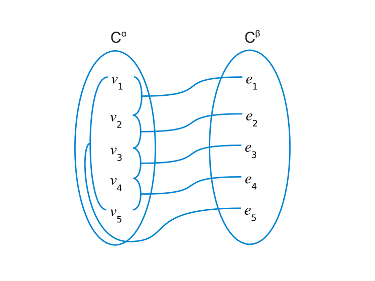
Figure 1: CSP encoding of the CGP on the graph $C_{5}$.

2.2 Structural Restrictions

In recent years, there has been a flurry of research into identifying tractable classes of classic CSP instances based on structural restrictions, that is, restrictions on the hypergraphs of CSP instances. Below, we present and discuss a few representative examples. In Sections 3 and 4, we will show how these techniques can be applied to CSP instance with global constraints. To present the various structural restrictions, we will use the framework of width functions, introduced by Adler adler-thesis .

Definition 7 (Hypergraph).

A hypergraph $\langle V,H\rangle$ is a set of vertices $V$ together with a set of hyperedges $H\subseteq\mathcal{P}(V)$.

Given a CSP instance $P=\langle V,C\rangle$, the hypergraph of $P$, denoted $\mathsf{hyp}(P)$, has vertex set $V$ together with a hyperedge $\mathcal{V}(\delta)$ for every $e[\delta]\in C$.

Definition 8 (Tree decomposition).

A tree decomposition of a hypergraph $\langle V,H\rangle$ is a pair $\langle T,\chi\rangle$ where $T$ is a tree and $\chi$ is a labelling function from nodes of $T$ to subsets of $V$, such that

1. for every $v\in V$, there exists a node $t$ of $T$ such that $v\in\chi(t)$,

2. for every hyperedge $h\in H$, there exists a node $t$ of $T$ such that $h\subseteq\chi(t)$, and

3. for every $v\in V$, the set of nodes $\{t\mid v\in\chi(t)\}$ induces a connected subtree of $T$.

Definition 9 (Width function).

Let $G=\langle V,H\rangle$ be a hypergraph. A width function on $G$ is a function $f:\mathcal{P}(V)-\{\emptyset\}\rightarrow\mathbb{R}^{+}$ that assigns a positive real number to every nonempty subset of vertices of $G$. A width function $f$ is monotone if $f(X)\leq f(Y)$ whenever $X\subseteq Y$.

Let $\langle T,\chi\rangle$ be a tree decomposition of $G$, and $f$ a width function on $G$. The $f$-width of $\langle T,\chi\rangle$ is $\max(\{f(\chi(t))\mid t\mbox{ node of }T\})$. The $f$-width of $G$ is the minimal $f$-width over all its tree decompositions.

In other words, a width function on a hypergraph $G$ tells us how to assign weights to nodes of tree decompositions of $G$.

Definition 10 (Treewidth).

Let $f(X)=|X|-1$. The treewidth $\mathsf{tw}(G)$ of a hypergraph $G$ is the $f$-width of $G$.

Let $G=\langle V,H\rangle$ be a hypergraph, and $X\subseteq V$. An edge cover of $X$ is any set of hyperedges $H^{\prime}\subseteq H$ that satisfies $X\subseteq\bigcup H^{\prime}$. The edge cover number $\rho(X)$ of $X$ is the size of the smallest edge cover of $X$. It is clear that $\rho$ is a width function.

Definition 11 ((adler-thesis, , Chapter 2)).

The generalized hypertree width $\mathsf{ghw}(G)$ of a hypergraph $G$ is the $\rho$-width of $G$.

Next, we define a relaxation of hypertree width known as fractional hypertree width, introduced by Grohe and Marx grohe-marx-frac-edge-cover .

Definition 12 (Fractional edge cover).

Let $G=\langle V,H\rangle$ be a hypergraph, and $X\subseteq V$. A fractional edge cover for $X$ is a function $\gamma:H\rightarrow[0,1]$ such that $\displaystyle\sum_{v\in h\in H}\gamma(h)\geq 1$ for every $v\in X$. We call $\displaystyle\sum_{h\in H}\gamma(h)$ the weight of $\gamma$. The fractional edge cover number $\rho^{*}(X)$ of $X$ is the minimum weight over all fractional edge covers for $X$. It is known that this minimum is always rational grohe-marx-frac-edge-cover . We furthermore define $\rho^{*}(G)=\rho^{*}(V)$.

Definition 13.

The fractional hypertree width $\mathsf{fhw}(G)$ of a hypergraph $G$ is the $\rho^{*}$-width of $G$.

For a class of hypergraphs $\mathcal{H}$ and a notion of width $\alpha$, we write $\alpha(\mathcal{H})$ for the maximal $\alpha$-width over the hypergraphs in $\mathcal{H}$. If this is unbounded we write $\alpha(\mathcal{H})=\infty$; otherwise $\alpha(\mathcal{H})<\infty$.

Bounding any of the above width measures by a constant can be used to guarantee tractability for classes of CSP instances where all constraints are table constraints.

Theorem 2.1 (Dalmau02:csp-tractability-cores ; Gottlob02:jcss-hypertree ; adler-gottlob-grohe-ghw ; grohe-marx-frac-edge-cover ; Marx2010-approx-frac-htw ).

Let $\mathcal{H}$ be a class of hypergraphs. For every $\alpha\in\{\mathsf{tw},\mathsf{ghw},\mathsf{fhw}\}$, any class of classic CSP instances whose hypergraphs are in $\mathcal{H}$ is tractable if $\alpha(\mathcal{H})<\infty$.

To go beyond fractional hypertree width, Marx DBLP:journals/corr/abs-0911-0801 recently introduced the concept of submodular width. This concept uses a set of width functions satisfying a condition (submodularity), and considers the $f$-width of a hypergraph for every such function $f$.

Definition 14 (Submodular width function).

Let $G=\langle V,H\rangle$ be a hypergraph. A width function $f$ on $G$ is edge-dominated if $f(h)\leq 1$ for every $h\in H$.

An edge-dominated width function $f$ on $G$ is submodular if for every pair of sets $X,Y\subseteq V$, we have $f(X)+f(Y)\geq f(X\cap Y)+f(X\cup Y)$.

Definition 15 (Submodular width).

Let $G$ be a hypergraph. The submodular width $\mathsf{subw}(G)$ of $G$ is the supremum of the $f$-widths of $G$ taken over all monotone, edge-dominated, submodular width functions $f$ on $G$.

For a class of hypergraphs $\mathcal{H}$, we write $\mathsf{subw}(\mathcal{H})$ for the maximal submodular width over the hypergraphs in $\mathcal{H}$. If this is unbounded we write $\mathsf{subw}(\mathcal{H})=\infty$; otherwise $\mathsf{subw}(\mathcal{H})<\infty$.

Unlike for fractional hypertree width and every other structural restriction discussed so far, the running time of the algorithm given by Marx for classic CSP instances with bounded submodular width has an exponential dependence on the number of vertices in the hypergraph of the instance. The class of classic CSP instances with bounded submodular width is therefore not known to be tractable. However, this class is what is called fixed-parameter tractable downey2012parameterized ; flum2006parameterized .

Definition 16 (Fixed-parameter tractable).

A parameterized problem instance is a pair $\langle k,P\rangle$, where $P$ is a problem instance, such as a CSP instance, and $k\in\mathbb{N}$ a parameter.

Let $S$ be a class of parameterized problem instances. We say that $S$ is fixed-parameter tractable (in ) if there is a computable function $f$ of one argument, as well as a constant $c$, such that every problem $\langle k,P\rangle\in S$ can be solved in time $O(f(k)\times|P|^{c})$.

The function $f$ can be arbitrary, but must only depend on the parameter $k$. For CSP instances, one possible parameterization is by the size of the hypergraph of an instance, measured by the number of vertices. Since the hypergraph of an instance has a vertex for every variable, for every CSP instance $P=\langle V,C\rangle$ we consider the parameterized instance $\langle|V|,P\rangle$.

Theorem 2.2 (DBLP:journals/corr/abs-0911-0801 ).

Let $\mathcal{H}$ be a class of hypergraphs. If $\mathsf{subw}(\mathcal{H})<\infty$, then a class of classic CSP instances whose hypergraphs are in $\mathcal{H}$ is in .

The three structural restrictions that we have just presented form a hierarchy grohe-marx-frac-edge-cover ; DBLP:journals/corr/abs-0911-0801 : For every hypergraph $G$, $\mathsf{subw}(G)\leq\mathsf{fhw}(G)\leq\mathsf{ghw}(G)\leq\mathsf{tw}(G)$.

As the example below demonstrates, Theorem 2.1 does not hold for CSP instances with arbitrary global constraints, even if we have a fixed, finite domain. The only exception is the restriction of Theorem 2.1 to treewidth, as bounded treewidth implies bounded arity for every hyperedge.

Example 4.

The -complete problem of 3-colourability Garey79:intractability is to decide, given a graph $\langle V,E\rangle$, whether the vertices $V$ can be coloured with three colours such that no two adjacent vertices have the same colour.

We may reduce this problem to a CSP with EGC constraints (cf. Example 1) as follows: Let $V$ be the set of variables for our CSP instance, each with domain $\{r,g,b\}$. For every edge $\langle v,w\rangle\in E$, we post an EGC constraint with scope $\{v,w\}$, parameterized by the function $K$ such that $K(r)=K(g)=K(b)=\{0,1\}$. Finally, we make the hypergraph of this CSP instance have low width by adding an EGC constraint with scope $V$ parameterized by the function $K^{\prime}$ such that $K^{\prime}(r)=K^{\prime}(g)=K^{\prime}(b)=\{0,\ldots,|V|\}$. This reduction clearly takes polynomial time, and the hypergraph $G$ of the resulting instance has $\mathsf{ghw}(G)=\mathsf{fhw}(G)=\mathsf{subw}(G)=1$.

As the constraint with scope $V$ allows all possible assignments, any solution to this CSP is also a solution to the 3-colourability problem, and vice versa.

Likewise, Theorem 2.2 does not hold for CSP instances with arbitrary global constraints if we allow the variables unbounded domain size, that is, change the above example to allow each variable its own set of colours. In other words, the structural restrictions cannot yield tractable classes of CSP instances with arbitrary global constraints. With that in mind, in the rest of the paper we will identify properties of extensionally represented constraints that these structural restrictions exploit to guarantee tractability. Then, we are going to look for restricted classes of global constraints that possess these properties. To do so, we will use the following definitions.

Definition 17 (Constraint catalogue).

A constraint catalogue is a set of global constraints. A CSP instance $\langle V,C\rangle$ is said to be over a constraint catalogue $\Gamma$ if for every $e[\delta]\in C$ we have $e[\delta]\in\Gamma$.

Definition 18 (Restricted CSP class).

Let $\Gamma$ be a constraint catalogue, and let $\mathcal{H}$ be a class of hypergraphs. We define $\textup{CSP}(\mathcal{H},\Gamma)$ to be the class of CSP instances over $\Gamma$ whose hypergraphs are in $\mathcal{H}$.

Definition 18 allows us to discuss classic CSP instances alongside instances with global constraints. Let $\mathbf{Ext}$ be the constraint catalogue containing all table global constraints. The classic CSP instances are then precisely those that are over $\mathbf{Ext}$. In particular, we can now restate Theorems 2.1 and 2.2 as follows.

Theorem 2.3.

Let $\mathcal{H}$ be a class of hypergraphs. For every $\alpha\in\{\mathsf{tw},\mathsf{ghw},\mathsf{fhw}\}$, the class of CSP instances $\textup{CSP}(\mathcal{H},\mathbf{Ext})$ is tractable if $\alpha(\mathcal{H})<\infty$. Furthermore, if $\mathsf{subw}(\mathcal{H})<\infty$ then $\textup{CSP}(\mathcal{H},\mathbf{Ext})$ is in .

3 Properties of Extensional Representation

We are going to start our investigation by considering fractional hypertree width in more detail. To obtain tractability for classic CSP instances of bounded fractional hypertree width, Grohe and Marx grohe-marx-frac-edge-cover use a bound on the number of solutions to a classic CSP instance, and show that this bound is preserved when we consider parts of a CSP instance. The following definition formalizes what we mean by “parts”, and is required to state the algorithm that Grohe and Marx use in their paper.

Definition 19 (Constraint projection).

Let $e[\delta]$ be a global constraint. The projection of $e[\delta]$ onto a set of variables $X\subseteq\mathcal{V}(\delta)$ is the constraint $\mathsf{pj}_{X}(e[\delta])$ such that $\mu\in\mathsf{pj}_{X}(e[\delta])$ if and only if there exists $\theta\in e[\delta]$ with $\theta|_{X}=\mu$.

For a CSP instance $P=\langle V,C\rangle$ and $X\subseteq V$ we define $\mathsf{pj}_{X}(P)=\langle X,C^{\prime}\rangle$, where $C^{\prime}$ is the set containing for every $e[\delta]\in C$ such that $X\cap\mathcal{V}(\delta)\not=\emptyset$ the constraint $\mathsf{pj}_{X\cap\mathcal{V}(\delta)}(e[\delta])$.

3.1 Algorithm for Enumerating All Solutions

The algorithm is given as Algorithm 1, and is essentially the usual recursive search algorithm for finding all solutions to a CSP instance by considering smaller and smaller sub-instances using constraint projections.

procedure EnumSolutions(CSP instance $P=\langle V,C\rangle$)$\triangleright$ Returns $\mathsf{sol}(P)$

     $\textup{Solutions}\leftarrow\emptyset$

     if $V=\emptyset$ then

         return $\{\bot\}$$\triangleright$ The empty assignment

     else

         $w\leftarrow\textup{chooseVar}(V)$$\triangleright$ Pick a variable from $V$

         $\Theta=\textup{EnumSolutions}(\mathsf{pj}_{V-\{w\}}(P))$

         for $\theta\in\Theta$ do

              for $a\in D(w)$ do

                  $\theta^{\prime}(w)=a$

                  if $\theta\oplus\theta^{\prime}$ is a solution to $P$ then

                       $\textup{Solutions.add}(\theta\oplus\theta^{\prime})$

                  end if

                  $\theta^{\prime}\leftarrow\bot$

              end for

         end for

     end if

     return Solutions

end procedure

Algorithm 1 Enumerate all solutions of a CSP instance

To show that Algorithm 1 does indeed find all solutions, we will use the following property of constraint projections.

Lemma 1.

Let $P=\langle V,C\rangle$ be a CSP instance. For every $X\subseteq V$, we have $\mathsf{sol}(\mathsf{pj}_{X}(P))\supseteq\pi_{X}(\mathsf{sol}(P))$.

Proof.

Given $P=\langle V,C\rangle$, let $X\subseteq V$ be arbitrary, and let $C^{\prime}=\{e[\delta]\in C\mid X\cap\mathcal{V}(\delta)\not=\emptyset\}$. For every $\theta\in\mathsf{sol}(P)$ and constraint $e[\delta]\in C^{\prime}$ we have that $\theta|_{\mathcal{V}(\delta)}\in e[\delta]$ since $\theta$ is a solution to $P$. By Definition 19, it follows that for every $e[\delta]\in C^{\prime}$, $\theta|_{X\cap\mathcal{V}(\delta)}\in\mathsf{pj}_{X\cap\mathcal{V}(\delta)}(e[\delta])$. Since the set of constraints of $\mathsf{pj}_{X}(P)$ is the least set containing for each $e[\delta]\in C^{\prime}$ the constraint $\mathsf{pj}_{X\cap\mathcal{V}(\delta)}(e[\delta])$, we have $\theta|_{X}\in\mathsf{sol}(\mathsf{pj}_{X}(P))$, and hence $\mathsf{sol}(\mathsf{pj}_{X}(P))\supseteq\pi_{X}(\mathsf{sol}(P))$. Since $X$ was arbitrary, the claim follows.

Theorem 3.1 (Correctness of Algorithm 1).

For every CSP instance $P$, we have that $\textup{EnumSolutions}(P)=\mathsf{sol}(P)$.

Proof.

The proof is by induction on the set of variables $V$ in $P$. For the base case, if $V=\emptyset$, the empty assignment is the only solution.

Otherwise, choose a variable $w\in V$, and let $X=V-\{w\}$. By induction, we can assume that $\textup{EnumSolutions}(\mathsf{pj}_{X}(P))=\mathsf{sol}(\mathsf{pj}_{X}(P))$. Since for every $\theta\in\mathsf{sol}(P)$ there exists $a\in D(w)$ such that $\theta=\theta|_{X}\cup\langle w,a\rangle$, and furthermore $\theta|_{X}\in\pi_{X}(\mathsf{sol}(P))$, it follows by Lemma 1 that $\theta|_{X}\in\mathsf{sol}(\mathsf{pj}_{X}(P))$. Since Algorithm 1 checks every assignment of the form $\mu\cup\langle w,a\rangle$ for every $\mu\in\mathsf{sol}(\mathsf{pj}_{X}(P))$ and $a\in D(w)$, it follows that $\textup{EnumSolutions}(P)=\mathsf{sol}(P)$.

The time required for this algorithm depends on three key factors, which we are going to enumerate and discuss below. Let

1. $s(P)$ be the maximum of the number of solutions to each of the instances $\mathsf{pj}_{W}(P)$, for $W\subseteq V$,

2. $c(P)$ be the maximum time required to check whether an assignment is a solution to $\mathsf{pj}_{W}(P)$, for $W\subseteq V$, and

3. $b(P)$ be the maximum time required to construct any instance $\mathsf{pj}_{W}(P)$, for $W\subseteq V$.

There are $|V|$ calls to EnumSolutions. For each call, we need $b(P)$ time to construct the projection, while the double loop takes at most $s(P)\times|D(w)|\times c(P)$ time. Therefore, letting $d=\max(\{|D(w)|\mid w\in V\})$, the running time of Algorithm 1 is bounded by $O\big{(}|V|\times(s(P)\times d\times c(P)+b(P))\big{)}$.

Since constructing the projection of a classic CSP instance can be done in polynomial time, and likewise checking that an assignment is a solution, the whole algorithm runs in polynomial time if $s(P)$ is a polynomial in the size of $P$. For fractional edge covers, Grohe and Marx show the following.

Lemma 2 (grohe-marx-frac-edge-cover ).

A classic CSP instance $P$ has at most $|P|^{\rho^{*}(\mathsf{hyp}(P))}$ solutions.

The reason for Lemma 2 is that fractional edge covers require the hypergraph to be quite dense, and also that the hyperedges grow with the number of vertices in the hypergraph. This result has since been shown to be optimal — a classic CSP instance has polynomially many solutions in its size if and only if it has bounded fractional edge cover number DBLP:journals/siamcomp/AtseriasGM13 .

Since fractional edge cover number is a monotone width function, it follows that for any instance $P=\langle V,C\rangle$ and $X\subseteq V$, $\rho^{*}(\mathsf{hyp}(\mathsf{pj}_{X}(P)))\leq\rho^{*}(\mathsf{hyp}(P))$. This claim follows from the fact that $\mathsf{pj}_{X}(P)$ projects every constraint down to $X$, and hence every hyperedge of $\mathsf{hyp}(P)$ down to $X$. Therefore, for classic CSP instances of bounded fractional edge cover number $s(P)$ is indeed polynomial in $|P|$. Grohe and Marx use this property to solve instances with bounded fractional hypertree width (and hence, bounded fractional edge cover number for every node in the corresponding tree decomposition) in polynomial time.

3.2 CSP Instances with Few Solutions in Key Places

As we have seen above, having few solutions for every projection of a CSP instance is a property that can be used to obtain tractable classes of classic CSP instances. More importantly, we have shown that this property allows us to find all solutions to a CSP instance $P$, even with global constraints, if we can build arbitrary projections of $P$ in polynomial time. In other words, with these two conditions we should be able to reduce instances with global constraints to classic instances in polynomial time. This, in turn, should allows us to apply the structural decomposition techniques discussed in Section 2.2 to such instances.

However, on reflection there is no reason why we should need few solutions for every projection. Instead, consider the following reduction.

Definition 20 (Partial assignment checking).

A global constraint catalogue $\Gamma$ allows partial assignment checking if there exists a polynomial $p(n)$ such that for any constraint $e[\delta]\in\Gamma$ we can decide in time $O(p(|\delta|))$ whether a given assignment $\theta$ to a set of variables $W\subseteq\mathcal{V}(\delta)$ is contained in an assignment that satisfies $e[\delta]$, i.e. whether there exists $\mu\in e[\delta]$ such that $\theta=\mu|_{W}$.

As an example, a catalogue that contains arbitrary EGC constraints (cf. Example 1) does not satisfy Definition 20, since checking whether an arbitrary EGC constraint has a satisfying assignment is -hard quimper04-gcc-npc . On the other hand, a catalogue that contains only EGC constraints whose cardinality sets are intervals does satisfy Definition 20 Regin96:aaai-generalized .

If a catalogue $\Gamma$ satisfies Definition 20, we can for any constraint $e[\delta]\in\Gamma$ build arbitrary projections of it, that is, construct the global constraint $\mathsf{pj}_{X}(e[\delta])$ for any $X\subseteq\mathcal{V}(\delta)$, in polynomial time. In the case of Algorithm 1, where we build projections of projections, we can do so by keeping a copy of the original constraint, and projecting that each time.

Definition 21 (Intersection variables).

Let $\langle V,C\rangle$ be a CSP instance. The set of intersection variables of any constraint $e[\delta]\in P$ is $\mathsf{iv}(\delta)=\bigcup\{\mathcal{V}(\delta)\cap\mathcal{V}(\delta^{\prime})\mid e^{\prime}[\delta^{\prime}]\in C-\{e[\delta]\}\}$.

Intersection variables are, in a sense, the only “interesting” variables of a constraint, as they are the ones interacting with the rest of the problem.

Definition 22 (Table constraint induced by a global constraint).

Let $P=\langle V,C\rangle$ be a CSP instance. For every $e[\delta]\in C$, let $\mu^{*}$ be the assignment to $\mathcal{V}(\delta)-\mathsf{iv}(\delta)$ that assigns a special value $*$ to every variable. The table constraint induced by $e[\delta]$ is $\mathsf{ic}(e[\delta])=e^{\prime}[\delta^{\prime}]$, where $\mathcal{V}(\delta^{\prime})=\mathcal{V}(\delta)$, and $\delta^{\prime}$ contains for every assignment $\theta\in\mathsf{sol}(\mathsf{pj}_{\mathsf{iv}(\delta)}(P))$ the assignment $\theta\oplus\mu^{*}$.

If every constraint in a CSP instance $P=\langle V,C\rangle$ allows partial assignment checking, then building $\mathsf{ic}(e[\delta])$ for any $e[\delta]\in C$ can be done in polynomial time when $|\mathsf{sol}(\mathsf{pj}_{X}(P))|$ is itself polynomial in the size of $P$ for every subset $X$ of $\mathsf{iv}(\delta)$. To do so, we can invoke Algorithm 1 on the instance $\mathsf{pj}_{\mathsf{iv}(\delta)}(P)$. The definition below expresses this idea.

Definition 23 (Sparse intersections).

A class of CSP instances $\mathcal{P}$ has sparse intersections if there exists a constant $c$ such that for every constraint $e[\delta]$ in any instance $P\in\mathcal{P}$, we have that for every $X\subseteq\mathsf{iv}(\delta)$, $|\mathsf{sol}(\mathsf{pj}_{X}(P))|<|P|^{c}$.

If a class of instances $\mathcal{P}$ has sparse intersections, and the instances are all over a constraint catalogue that allows partial assignment checking, then we can for every constraint $e[\delta]$ of any instance from $\mathcal{P}$ construct $\mathsf{ic}(e[\delta])$ in polynomial time. While this definition considers the instance as a whole, one special case of it is the case where every constraint has few solutions in the size of its description, that is, there is a constant $c$ and the constraints are drawn from a catalogue $\Gamma$ such that for every $e[\delta]\in\Gamma$, we have that $|\{\mu\mid\mu\in e[\delta]\}|<|\delta|^{c}$.

Note that the problem of checking whether a class of CSP instances satisfies Definition 23 for a given $c$ is, in general, hard. To see this, consider the special case of checking whether a global constraint $e[\delta]$ has any satisfying assignments at all. Letting $\delta$ be a SAT instance, that is, a propositional formula, and $e$ an algorithm that checks whether an assignment to $\mathcal{V}(\delta)$ satisfies the formula makes this an -hard problem to solve.

More generally, consider an arbitrary problem in . By definition, there is a polynomial-time algorithm that can check if a proposed solution to such a problem is correct. By treating the algorithm as the constraint type $e$, and the problem instances as descriptions $\delta$, with a variable in $\mathcal{V}(\delta)$ for each bit of the solution, it becomes clear that every problem in corresponds to a class of global constraints. The fact that global constraints have this much expressive power will be explored further in Section 4.

Despite such bad news, however, it is not always difficult to recognise constraints with polynomially many satisfying assignments. A trivial example would be table constraints. For a less trivial example, consider the constraint $C^{\beta}$ from Example 3, where the number of satisfying assignments is bounded by a polynomial with exponent $\beta$ (cf. the discussion after Corollary 1 for a detailed analysis).

For a more general example, consider a family of constraints that satisfy Definition 20. To check whether the number of solutions to a constraint from such a family is bounded by $|\delta|^{c}$ for a fixed $c$ in polynomial time, we can use Algorithm 1, stopping it if the number of partial assignments that extend to solutions exceeds the bound. Since we can check whether a partial assignment extends to a solution in polynomial time by Definition 20, we are also guaranteed an answer in polynomial time.

Armed with these definitions, we can now state the following result.

Theorem 3.2.

Let $\mathcal{P}$ be a class of CSP instances over a catalogue that allows partial assignment checking. If $\mathcal{P}$ has sparse intersections, then we can in polynomial time reduce any instance $P\in\mathcal{P}$ to a classic CSP instance $P_{CL}$ with $\mathsf{hyp}(P)=\mathsf{hyp}(P_{CL})$, such that $P_{CL}$ has a solution if and only if $P$ does.

Proof.

Let $P=\langle V,C\rangle$ be an instance from such a class $\mathcal{P}$. For each $e[\delta]\in C$, $P_{CL}$ will contain the table constraint $\mathsf{ic}(e[\delta])$ from Definition 22. Since $P$ is over a catalogue that allows partial assignment checking, and $\mathcal{P}$ has sparse intersections, computing $\mathsf{ic}(e[\delta])$ can be done in polynomial time by invoking Algorithm 1 on $\mathsf{pj}_{\mathsf{iv}(\delta)}(P)$.

By construction, $\mathsf{hyp}(P)=\mathsf{hyp}(P_{CL})$. All that is left to show is that $P_{CL}$ has a solution if and only if $P$ does. Let $\theta$ be a solution to $P=\langle V,C\rangle$. For every $e[\delta]\in C$, we have that $\theta|_{\mathsf{iv}(\delta)}\in\mathsf{pj}_{\mathsf{iv}(\delta)}(P)$ by Definitions 19 and 21, and the assignment $\mu$ that assigns the value $\theta(v)$ to each $v\in\displaystyle\bigcup_{e[\delta]\in C}\mathsf{iv}(\delta)$, and $*$ to every other variable is therefore a solution to $P_{CL}$.

In the other direction, if $\theta$ is a solution to $P_{CL}$, then $\theta$ satisfies $\mathsf{ic}(e[\delta])$ for every $e[\delta]\in C$. By Definition 22, this means that $\theta|_{\mathsf{iv}(\delta)}\in\mathsf{sol}(\mathsf{pj}_{\mathsf{iv}(\delta)}(P))$, and by Definition 19, there exists an assignment $\mu^{e[\delta]}$ with $\mu^{e[\delta]}|_{\mathsf{iv}(\delta)}=\theta|_{\mathsf{iv}(\delta)}$ that satisfies $e[\delta]$. By Definition 21, the variables not in $\mathsf{iv}(\delta)$ do not occur in any other constraint in $P$, so we can combine all the assignments $\mu^{e[\delta]}$ to form a solution $\mu$ to $P$ such that for $e[\delta]\in C$ and $v\in\mathcal{V}(\delta)$ we have $\mu(v)=\mu^{e[\delta]}(v)$.

From Theorem 3.2, we get tractable and fixed-parameter tractable classes of CSP instances with global constraints, in particular by applying Theorem 2.3.

Corollary 1.

Let $\mathcal{H}$ be a class of hypergraphs, and $\Gamma$ a catalogue that allows partial assignment checking. If $\textup{CSP}(\mathcal{H},\Gamma)$ has sparse intersections, then $\textup{CSP}(\mathcal{H},\Gamma)$ is tractable or in if $\textup{CSP}(\mathcal{H},\mathbf{Ext})$ is.

Proof.

Let $\mathcal{H}$ and $\Gamma$ be given. By Theorem 3.2, we can reduce any $P\in\textup{CSP}(\mathcal{H},\Gamma)$ to an instance $P_{CL}\in\textup{CSP}(\mathcal{H},\mathbf{Ext})$ in polynomial time. Since $P_{CL}$ has a solution if and only if $P$ does, tractability or fixed-parameter tractability of $\textup{CSP}(\mathcal{H},\mathbf{Ext})$ implies the same for $\textup{CSP}(\mathcal{H},\Gamma)$.

To illustrate the above result, consider again the connected graph partition problem (Problem 1). This problem is -complete (Garey79:intractability, , p. 209), even for fixed $\alpha\geq 3$. However, note that when $\beta$ is fixed, we can solve the problem in polynomial time, by successively guessing sets $E^{\prime}$, with $|E^{\prime}|\leq\beta$, of broken edges, and checking whether the connected components of the graph $\langle V,E-E^{\prime}\rangle$ all have $\alpha$ or fewer vertices. The number of such sets $E^{\prime}$ is bounded by $\displaystyle\sum_{i=1}^{\beta}\binom{|E|}{i}\leq(|E|+1)^{\beta}$, which is polynomial if $\beta$ is fixed. As we show below, this argument can be seen as a special case of Theorem 3.2. To simplify the analysis, we assume without loss of generality that $\alpha<|V|$, which means that any solution has at least one broken edge.

We claim that if $\beta$ is fixed, then the constraint $C^{\beta}=e^{\beta}[\delta^{\beta}]$ allows partial assignment checking, and has only a polynomial number of satisfying assignments. The latter implies that for any instance $P$ of the CGP, $|\mathsf{sol}(\mathsf{pj}_{\mathsf{iv}(\delta^{\beta})}(P))|$ is polynomial in the size of $P$ for every subset of $\mathsf{iv}(\delta^{\beta})$. Furthermore, we will show that for the constraint $C^{\alpha}=e^{\alpha}[\delta^{\alpha}]$, we also have that $|\mathsf{sol}(\mathsf{pj}_{\mathsf{iv}(\delta^{\alpha})}(P))|$ is polynomial in the size of $P$. That $C^{\alpha}$ allows partial assignment checking can be seen by noting that each variable in $\mathcal{V}(\delta^{\alpha})$ has a domain value for every vertex in the underlying graph. Therefore, given a partial assignment to $\mathcal{V}(\delta^{\alpha})$, we can check that no value is assigned more than $\alpha$ times. If yes, this assignment can be extended to a full one by assigning each remaining variable a domain value not yet assigned to any variable.

First, we show that the number of satisfying assignments to $C^{\beta}$ is limited. Since $C^{\beta}$ limits the number of ones in any solution to $\beta$, the number of satisfying assignments to this constraint is the number of ways to choose up to $\beta$ variables to be assigned one. This is bounded by $\displaystyle\sum^{\beta}_{i=1}\binom{|E|}{i}\leq(|E|+1)^{\beta}$, and so we can generate them all in polynomial time. This argument also implies that we can perform partial assignment checking, simply by looking at the generated assignments.

Now, let $\theta$ be such a solution. How many solutions to $P$ contain $\theta$? Every constraint on $\{u,v,e\}$ with $\theta(e)=1$ allows at most $|V|^{2}$ assignments, and there are at most $\beta$ such constraints. So far we therefore have at most $(|E|+1)^{\beta}\times|V|^{2\beta}$ assignments.

On the other hand, a ternary constraint with $\theta(e)=0$ requires $\theta(u)=\theta(v)$. Consider the graph $G_{0}$ containing for every constraint on $\{u,v,e\}$ with $\theta(e)=0$ the vertices $u$ and $v$ as well as the edge $\{u,v\}$. Since the original graph was connected, every connected component of $G_{0}$ contains at least one vertex which is in the scope of some constraint with $\theta(e)=1$. Therefore, since equality is transitive, each connected component of $G_{0}$ allows at most one assignment for each of the $(|E|+1)^{\beta}\times|V|^{2\beta}$ assignments to the other variables of $P$. We therefore get a total bound of $(|E|+1)^{\beta}\times|V|^{2\beta}$ on the total number of solutions to $P$, and hence to $\mathsf{pj}_{\mathsf{iv}(\delta^{\alpha})}(P)$.

The hypergraph of any CSP instance $P$ encoding the CGP has two hyperedges covering the whole problem, so the hypertree width of this hypergraph is two. Therefore, Corollaries 1 and 2.1 apply and yield tractability for fixed $\beta$.

3.3 Back Doors

If a class of CSP instances includes constraints from a catalogue that is not known to allow partial assignment checking, we may still obtain tractability in some cases by applying the notion of a back door set. A (strong) back door set gaspers-backdoors ; Williams03backdoorsto is a set of variables in a CSP instance that, when assigned, make the instance easy to solve. Below, we are going to adapt this notion to individual constraints.

Definition 24 (Back door).

Let $\Gamma$ be a global constraint catalogue. A back door for a constraint $e[\delta]\in\Gamma$ is any set of variables $W\subseteq\mathcal{V}(\delta)$ (called a back door set) such that we can decide in polynomial time whether a given assignment $\theta$ to a set of variables $\mathcal{V}(\theta)\supseteq W$ is contained in an assignment that satisfies $e[\delta]$, i.e. whether there exists $\mu\in e[\delta]$ such that $\mu|_{\mathcal{V}(\theta)}=\theta$.

Trivially, for every constraint $e[\delta]$ the set of variables $\mathcal{V}(\delta)$ is a back door set, since by Definition 4 we can always check in polynomial time if an assignment to $\mathcal{V}(\delta)$ satisfies the constraint $e[\delta]$.

The key point about back doors is that given a catalogue $\Gamma$, adding to each $e[\delta]\in\Gamma$ with back door set $W$ an arbitrary set of assignments to $W$ produces a catalogue $\Gamma^{\prime}$ that allows partial assignment checking. Adding a set of assignments $\Theta$ means to add $\Theta$ to the description, and modify the algorithm $e$ to only accept an assignment if it contains a member of $\Theta$ in addition to previous requirements. Furthermore, given a CSP instance $P$ containing $e[\delta]$, as long as $\Theta\supseteq\pi_{W}(\mathsf{sol}(P))$, adding $\Theta$ to $e[\delta]$ produces an instance that has exactly the same solutions. This point leads to the following definition.

Definition 25 (Sparse back door cover).

Let $\Gamma_{PAC}$ be a catalogue that allows partial assignment checking and $\Gamma_{BD}$ a catalogue. For every instance $P=\langle V,C\rangle$ over $\Gamma_{PAC}\cup\Gamma_{BD}$, let $P\cap\Gamma_{PAC}$ be the instance with constraint set $C^{\prime}=C\cap\Gamma_{PAC}$ and set of variables $\bigcup\{V\cap\mathcal{V}(\delta)\mid e[\delta]\in C^{\prime}\}$.

A class of CSP instances $\mathcal{P}$ over $\Gamma_{PAC}\cup\Gamma_{BD}$ has sparse back door cover if there exists a constant $c$ such that for every instance $P=\langle V,C\rangle\in\mathcal{P}$ and constraint $e[\delta]\in C$, if $e[\delta]\not\in\Gamma_{PAC}$, then there exists a back door set $W$ for $e[\delta]$, findable in time polynomial in $|P|$, such that $|\mathsf{sol}(\mathsf{pj}_{X}(P\cap\Gamma_{PAC}))|\leq|P|^{c}$ for every $X\subseteq W$.

Sparse back door cover means that for each constraint that is not from a catalogue that allows partial assignment checking, we can in polynomial time get a set of assignments $\Theta$ for its back door set using Algorithm 1, and so turn this constraint into one that does allow partial assignment checking. This operation preserves the solutions of the instance that contains this constraint.

Theorem 3.3.

If a class of CSP instance $\mathcal{P}$ has sparse back door cover, then we can in polynomial time reduce any instance $P\in\mathcal{P}$ to an instance $P^{\prime}$ such that $\mathsf{hyp}(P)=\mathsf{hyp}(P^{\prime})$ and $\mathsf{sol}(P)=\mathsf{sol}(P^{\prime})$. Furthermore, the class of instances $\{P^{\prime}\mid P\in\mathcal{P}\}$ is over a catalogue that allows partial assignment checking.

Proof.

Let $P=\langle V,C\rangle\in\mathcal{P}$. We construct $P^{\prime}$ by adding to every $e[\delta]\in C$ such that $e[\delta]\not\in\Gamma_{PAC}$, with back door set $W$, the set of assignments $\mathsf{sol}(\mathsf{pj}_{W}(P\cap\Gamma_{PAC}))$, which we can obtain using Algorithm 1. By Definition 25, we have for every $X\subseteq W$ that $|\mathsf{sol}(\mathsf{pj}_{W}(P\cap\Gamma_{PAC}))|\leq|P|^{c}$, so Algorithm 1 takes polynomial time since $\Gamma_{PAC}$ does allow partial assignment checking.

It is clear that $\mathsf{hyp}(P^{\prime})=\mathsf{hyp}(P)$, and since $\mathsf{sol}(\mathsf{pj}_{W}(P\cap\Gamma_{PAC}))\supseteq\pi_{W}(\mathsf{sol}(P))$, the set of solutions stays the same, i.e. $\mathsf{sol}(P^{\prime})=\mathsf{sol}(P)$. Finally, since we have replaced each constraint $e[\delta]$ in $P$ that was not in $\Gamma_{PAC}$ by a constraint that does allow partial assignment checking, it follows that $P^{\prime}$ is over a catalogue that allows partial assignment checking.

One consequence of Theorem 3.3 is that we can sometimes apply Theorem 3.2 to a CSP instance that contains a constraint for which checking if a partial assignment can be extended to a satisfying one is hard. We can do so when the variables of that constraint are covered by the variables of other constraints that do allow partial assignment checking — but only if the instance given by those constraints has few solutions.

As a concrete example of this, consider again the encoding of the CGP that we gave in Example 3. The variables of constraint $C^{\alpha}$ are entirely covered by the instance $P^{\prime}$ obtained by removing $C^{\alpha}$. As the entire set of variables of a constraint is a back door set for it, and the instance $P^{\prime}$ has few solutions (cf. the discussion after Theorem 3.2), this class of instances has sparse back door cover. As such, the constraint $C^{\alpha}$ could, in fact, be arbitrary without affecting the tractability of this problem. In particular, the requirement that $C^{\alpha}$ allows partial assignment checking can be dropped.

4 Subproblem Decompositions

To generalize Theorem 3.2, consider the fact that our definition of a global constraint allows us to view a CSP instance $\langle V,C\rangle$ as a single constraint $e[\delta]$, by letting $\delta$ contain the set of constraint $C$, and setting $\mathcal{V}(\delta)=V$. The algorithm $e$ then checks if an assignment satisfies all constraints. Of course, such a constraint encodes an -complete problem, but this is no different from e.g. the EGC constraint quimper04-gcc-npc (cf. Example 1). With this in mind, in this section we are going to investigate what happens if a CSP instance is split up into a set of smaller instances.

Splitting up a (classic) CSP instance into smaller instances has previously been considered by Cohen and Green guarded-decomp-CG . They use a very general framework of guarded decompositions CohenUnifTract to define what they call “typed guarded decompositions”. This notion allows them to obtain a tractability result for a CSP instance that can be split into smaller instances drawn from known tractable classes.

In this section, we are going to adapt the notions defined in Section 3.2 to work with CSP instances rather than single constraints. Then, in Section 4.1, we will show how the result of Cohen and Green can be derived as a special case of Corollary 2.

Definition 26 (CSP subproblem).

Given two CSP instances $P=\langle V,C\rangle$ and $P^{\prime}=\langle V^{\prime},C^{\prime}\rangle$, we say that $P^{\prime}$ is a subproblem of $P$ if $C^{\prime}\subseteq C$.

In other words, a subproblem of a CSP instance is given by a subset of the constraints in that instance. In guarded-decomp-CG , Cohen and Green call a subproblem a component of $P$.

Definition 27 (CSP union).

Let $Q_{1}=\langle V_{1},C_{1}\rangle$ and $Q_{2}=\langle V_{2},C_{2}\rangle$ be two CSP instances. The union of $Q_{1}$ and $Q_{2}$ is the instance $Q_{1}\sqcup Q_{2}=\langle V_{1}\cup V_{2},C_{1}\cup C_{2}\rangle$.

Definition 28 (Subproblem decomposition).

Let $P$ be a CSP instance. A set $S$ of subproblems of $P$ is a subproblem decomposition of $P$ if $\bigsqcup S=P$.

A subproblem decomposition of a CSP instance is proper if no element of the decomposition is a subproblem of any other.

A subproblem decomposition of an instance $P$, then, is a set of subproblems that together contain all the constraints and variables of $P$. Note that a constraint may occur in more than one subproblem in a decomposition.

Below, we shall assume that all subproblem decompositions are proper. Since subproblems are given by subsets of constraints, the solutions to a CSP instance can be turned into solutions for any subproblem by projecting out the variables not part of the subproblem. Therefore, solving a subproblem $P$ that contains another subproblem $P^{\prime}$ also solves $P^{\prime}$, making $P^{\prime}$ redundant.

Example 5.

Let $P=\langle V,C\rangle$ be a CSP instance. A very simple subproblem decomposition of $P$ would be $\{\langle\mathcal{V}(\delta),e[\delta]\rangle\mid e[\delta]\in C\}$, that is, every constraint of $P$ is a separate subproblem. This subproblem decomposition is clearly proper.

Example 6.

Consider a family of CSP instances on the set of boolean variables $\{x_{i},y_{i},z_{i}\mid 1\leq i\leq n\in\{4,6,8,\ldots\}\}$, with the following constraints: An EGC constraint $A$ on $\{x_{1},\ldots,x_{n}\}$ with $K(1)=4$ and $K(0)=\{0,\ldots,n\}$. A second EGC constraint $B$, on $\{y_{1},\ldots,y_{n},z_{1},\ldots,z_{n}\}$ with $K(1)=K(0)=\{n\}$, and binary constraints on each pair $\{x_{i},y_{i}\}$ enforcing equality. A possible subproblem decomposition for an instance from this family would be $\{P,Q\}$, where $P$ contains $A$ as well as the binary constraints, and $Q$ contains the constraint $B$. This family is depicted in Figure 2, with $P$ containing the constraints marked by solid lines, and $Q$ the constraint marked by a dashed line.

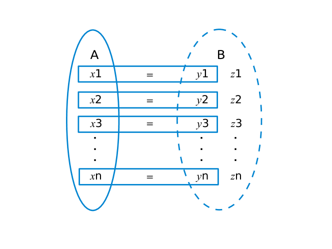
Figure 2: Family of instances from Example 6 with decomposition $\{P,Q\}$. Subproblem $P$ marked with solid lines and $Q$ with a dashed line.

Viewing subproblems as constraints and a subproblem decomposition $S$ as a CSP instance $\langle\mathcal{V}(\bigsqcup S),S\rangle$, we have $\mathsf{sol}(\langle\mathcal{V}(\bigsqcup S),S\rangle)=\mathsf{sol}(\bigsqcup S)$, since every constraint is in some subproblem. As such, we will treat $S$ as a CSP instance when it is convenient to simplify notation.

Using Definition 28, we can treat any set of CSP instances $S$ as a subproblem decomposition of the instance $\bigsqcup S$. With that in mind, whenever we say that $S$ is a subproblem decomposition without specifying what it is a decomposition of, we mean that $S$ is a decomposition of the CSP instance $\bigsqcup S$.

Definition 29 (CSP instances given by subproblem decompositions).

Let $\mathcal{F}$ be a family of subproblem decompositions. We define $\textup{CSP}(\mathcal{F})$ to be the class of CSP instances $\{\bigsqcup S\mid S\in\mathcal{F}\}$.

Definition 30 (Hypergraph of a subproblem decomposition).

Let $S$ be a subproblem decomposition. The hypergraph of $S$, denoted $\mathsf{hyp}(S)$, has vertex set $\mathcal{V}(\bigsqcup S)$ and set of hyperedges $\{\mathcal{V}(P)\mid P\in S\}$.

For a family $\mathcal{F}$ of subproblem decompositions, let $\mathsf{hyp}(\mathcal{F})=\{\mathsf{hyp}(S)\mid S\in\mathcal{F}\}$.

Since a CSP instance can be seen as a global constraint, Definition 20 (partial assignment checking) and Definition 23 (sparse intersections) carry over unchanged. To apply them to a family of subproblem decompositions $\mathcal{F}$, we need only consider the catalogue $\bigcup\mathcal{F}$ in both cases.

One way of interpreting Definition 20 for a catalogue of CSP instances is that every instance has been drawn from a tractable class — not necessarily the same one, as long as these classes all allow us to check in polynomial time whether a partial assignment extends to a solution. Most known tractable classes of CSP instances have this property; in particular, all the classes discussed in Section 2.2 have it. To see this, note that a partial assignment can be seen as a set of constraints on one variable each, and adding such hyperedges to a hypergraph does not change its tree, hypertree, or submodular width. On the other hand, tractable classes defined by restricting the allowed assignments of a constraint, rather than the hypergraph, are usually preserved by adding a constraint with only one assignment Cohen-comp-lang-handbook .

To illustrate how these definitions apply to subproblem decompositions, consider the following example.

Example 7.

Recall the family of subproblem decompositions in Example 6. For a decomposition $S=\{P,Q\}$ from this family, the set of intersection vertices for both subproblems is $\{y_{1},\ldots,y_{n}\}$. Furthermore, the EGC constraint $A$ requires that there are exactly $4$ variables assigned $1$ among $\{x_{1},\ldots,x_{n}\}$, so there are $\binom{n}{4}$ satisfying assignments for this constraint. The equality constraints ensure that this is the number of solutions to the whole subproblem $P$, so for every $X\subseteq\{y_{1},\ldots,y_{n}\}$ we have that $|\mathsf{sol}(\mathsf{pj}_{X}(S))|\leq\binom{n}{4}$. Therefore, this family of subproblem decompositions has sparse intersections.

We can now derive a straightforward generalization of Theorem 3.2.

Theorem 4.1.

Let $\mathcal{F}$ be a family of subproblem decompositions that allows partial assignment checking. If $\mathcal{F}$ has sparse intersections, then we can in polynomial time reduce any subproblem decomposition $S\in\mathcal{F}$ to a classic CSP instance $P$ with $\mathsf{hyp}(P)=\mathsf{hyp}(S)$, such that $P$ has a solution if and only if $S$ does.

Proof.

As subproblems can be seen as global constraints, the proof follows directly from Theorem 3.2.

Corollary 2.

Let $\mathcal{F}$ be a family of subproblem decompositions that allows partial assignment checking and has sparse intersections. If $\textup{CSP}(\mathsf{hyp}(\mathcal{F}),\mathbf{Ext})$ is tractable or in , then so is $\textup{CSP}(\mathcal{F})$.

Proof.

Let $\mathcal{F}$ be given. By Theorem 4.1, we can reduce any subproblem decomposition $S\in\mathcal{F}$ to an instance $P\in\textup{CSP}(\mathsf{hyp}(\mathcal{F}),\mathbf{Ext})$ in polynomial time. Since $P$ has a solution if and only if $S$ does, tractability of $\textup{CSP}(\mathsf{hyp}(\mathcal{F}),\mathbf{Ext})$ implies the same for $\textup{CSP}(\mathcal{F})$.

To illustrate this result, recall Example 6. From Example 7, we know that this family of subproblem decompositions has sparse intersections. Furthermore, both subproblem allow partial assignment checking, as the EGC constraints both have interval cardinality sets Regin96:aaai-generalized , and the equality constraints of subproblem $P$ can always be satisfied. Therefore, Corollary 2 applies to this problem.

4.1 Applying Corollary 2

We are now ready to discuss the result of Cohen and Green mentioned at the beginning of Section 4, and to show how it can be derived as a special case of our result. First, we need to define guarded decompositions.

Definition 31 (Guarded decomposition).

A guarded block of a hypergraph $G$ is a pair $\langle\lambda,\chi\rangle$ where the guard $\lambda$ is a subset of the hyperedges of $G$, and the block, $\chi$, is a subset of $\bigcup\lambda$.

For every classic CSP instance $P$ and every guarded block $\langle\lambda,\chi\rangle$ of $\mathsf{hyp}(P)$, we define the constraint generated by $P$ on $\langle\lambda,\chi\rangle$ to be the projection onto $\chi$ of the join of all the constraints of $P$ whose scopes are in $\lambda$.

A set of of guarded blocks $\Theta$ of a hypergraph $G$ is a guarded decomposition of $G$ if for every $P\in\textup{CSP}(\{G\},\mathbf{Ext})$, the CSP instance over the same variables as $P$ with constraints generated by the blocks in $\Theta$ has the same solutions as $P$.

A guarded decomposition is acyclic if the hypergraph having the union of the blocks $\chi$ as vertices, and each $\chi$ as a hyperedge, is acyclic.

Cohen and Green then introduce a mapping $\mu$ from the constraints of a CSP instance $P$ to nonempty sets of elements of a guarded decomposition of $\mathsf{hyp}(P)$. They demand that

1. For each guarded block $\langle\lambda,\chi\rangle$ and hyperedge in $\lambda$, $\mu$ assigns at least one constraint with that scope to this guarded block,

2. that the set of guarded blocks $\mu$ assigns to a constraint $c$ contains the scope of $c$ in all the guards, and finally

3. that at least one of the guarded blocks assigned to $c$ contains the variables of the scope of $c$ in the block.

Note that, taken together, the conditions above mean that the mapping $\mu$ turns each guarded block of the decomposition into a subproblem, and the whole decomposition into a subproblem decomposition, since each guarded block is assigned a set of constraints, and each constraint is assigned to a guarded block.

Furthermore, they introduce two more notions. A type is a polynomial-time algorithm for solving a set of CSP instances. A typed guarded decomposition is one where each guarded block $\beta$ is assigned a type, and the CSP instance given by the set of constraints assigned to $\beta$ is a member of the assigned type. This is almost Definition 20, however, there is no provision for solving a problem with some variables assigned.

Finally, a guarded decomposition $\Theta$ is $k$-separated if for every guarded block $\langle\lambda,\chi\rangle$ there exists a set of hyperedges $\epsilon$, with $|\epsilon|\leq k$, such that for each guarded block $\langle\lambda_{2},\chi_{2}\rangle\in\Theta-\{\lambda,\chi\}$ we have that $\chi\cap\chi_{2}\subseteq\bigcup\epsilon$. Observe that when $k$ is fixed, the intersection variables of each subproblem are covered by a fixed number of table constraints, and hence that the number of possible solutions is bounded by the size of the join of these constraints. It follows that the intersections are sparse as per Definition 23.

They then proceed to show that for fixed $k$, a CSP instance with a $k$-separated, acyclic typed guarded decomposition can be solved in polynomial time, under the condition that the types can handle problems with some variables assigned specific values.

The last condition is precisely what we need for partial assignment checking. Therefore, since the decomposition is required to be acyclic, their result satisfies the conditions of Corollary 2. Note, however, that since there are other ways to obtain sparse intersections, Corollary 2 is a more general result even for classic CSP instances.

5 Weighted CSP

Having few solutions in key parts of a CSP instance has turned out to be a property we can exploit to obtain tractability. In this section, we are going to apply this property to an extension of the CSP framework called weighted CSP instances gottlob-etal-tractable-optimization ; degivry06 , where every constraint assigns a cost to every satisfying assignment, and we would like to find a solution with smallest cost. This type of CSP is itself a special case of the more general valued CSP framework schiex95vcsp ; standa-vcsp , where every constraint is specified by a function that assigns a cost to every possible assignment for the variables of that constraint. The reason for considering weighted, rather than valued, CSP, is that weighted (table) constraints list every satisfying assignment along with the costs, while a valued constraint is given by a function from assignments to values. The representation of a valued constraint is thus much more compact, and the notion of a satisfying assignment is no longer defined.

Definition 32 (Weighted constraint).

A weighted global constraint $e[\delta]$ is a global constraint that assigns to each $\theta\in e[\delta]$ a value $\mathsf{cost}(e[\delta],\theta)$ from $\mathbb{Q}$.

The size of a weighted global constraint $e[\delta]$ is given by the sum of $|\delta|$ and the size of the bit representation for each cost.

In other words, the number of bits needed to represent the costs of all the satisfying assignments is part of a weighted constraint’s size.

Definition 33 (WCSP instance).

A WCSP instance is a pair $P=\langle V,C\rangle$, where $V$ is a set of variables and $C$ a set of weighted constraints. An assignment is a solution to $P$ if it satisfies every constraint in $C$, and we denote the set of all solutions to $P$ by $\mathsf{sol}(P)$.

For every solution $\theta$ to $P$ we define $\mathsf{cost}(P,\theta)=\displaystyle\sum_{e[\delta]\in C}\mathsf{cost}(e[\delta],\theta|_{\mathcal{V}(\delta)})$. An assignment $\theta$ is an optimal solution to $P$ if and only if it is a solution to $P$ with the smallest cost, i.e. $\mathsf{cost}(P,\theta)=\min(\{\mathsf{cost}(P,\theta^{\prime})\mid\theta^{\prime}\in\mathsf{sol}(P)\})$.

As is commonly done with optimization problems in complexity theory, below we consider the decision problem associated with WCSP instances.

Definition 34 (WCSP decision problem).

Given a WCSP instance $P$ and $k\in\mathbb{Q}$, the WCSP decision problem is to decide whether $P$ has a solution $\theta$ with $\mathsf{cost}(P,\theta)\leq k$.

As for CSP instances, a classic WCSP instance is one where all constraints are table global constraints. As an example of known tractability results for classic WCSP instances, consider the theorem below.

Theorem 5.1 (gottlob-etal-tractable-optimization ).

Let $\mathcal{H}$ be a class of hypergraphs. If $\mathsf{ghw}(\mathcal{H})<\infty$, then a class of classic WCSP instances whose hypergraphs are in $\mathcal{H}$ is tractable.

Since we are free to ignore the costs a weighted constraint puts on assignments and treat it as an “ordinary” constraint, definitions of subproblems and subproblem decompositions carry over unchanged. Note that since the WCSP decision problem is clearly in , we can view a WCSP instance as a weighted global constraint. Therefore, Definition 20 will now be subtly different.

Definition 35 (Weighted part. assignment checking).

A weighted constraint catalogue $\Gamma$ allows partial assignment checking if for any weighted constraint $e[\delta]\in\Gamma$ we can decide in polynomial time, given an assignment $\theta$ to a set of variables $W\subseteq\mathcal{V}(\delta)$ and $k\in\mathbb{Q}$, whether $\theta$ is contained in an assignment that satisfies $e[\delta]$ and has cost at most $k$, i.e. whether there exists $\mu\in e[\delta]$ such that $\theta=\mu|_{W}$ and $\mathsf{cost}(e[\delta],\mu)\leq k$.

In other words, given a partial assignment we need to be able to solve the WCSP decision problem for our constraint in polynomial time. Note also that doing so allows us to find the minimum cost among the assignments that contain our partial assignment by binary search. This will be needed in order to construct projections of a weighted global constraint. To define the projection of a weighted constraint, we need to alter Definition 19 to take costs into account.

Definition 36 (Weighted constraint projection).

Let $e[\delta]$ be a weighted constraint. The projection of $e[\delta]$ onto a set of variables $X\subseteq\mathcal{V}(\delta)$ is the constraint $\mathsf{pj}_{X}(e[\delta])$ such that $\mu\in\mathsf{pj}_{X}(e[\delta])$ if and only if there exists $\theta\in e[\delta]$ with $\theta|_{X}=\mu$. The cost of an assignment $\theta\in\mathsf{pj}_{X}(e[\delta])$ is $\mathsf{cost}(\mathsf{pj}_{X}(e[\delta]),\theta)=\min(\{\mathsf{cost}(e[\delta],\mu)\mid\mu\in e[\delta]\mbox{ and }\mu|_{X}=\theta\})$.

For a WCSP instance $P=\langle V,C\rangle$ and $X\subseteq V$ we define $\mathsf{pj}_{X}(P)=\langle X,C^{\prime}\rangle$, where $C^{\prime}$ is the least set containing for every $e[\delta]\in C$ such that $X\cap\mathcal{V}(\delta)\not=\emptyset$ the constraint $\mathsf{pj}_{X\cap\mathcal{V}(\delta)}(e[\delta])$.

Definition 37 (Weighted table constraint induced by a subproblem).

Let $S$ be a subproblem decomposition. For every $T\in S$, let $\mu^{*}$ be the assignment to $\mathcal{V}(T)-\mathsf{iv}(T)$ that assigns a special value $*$ to every variable. The weighted table constraint induced by $T$ is $\mathsf{ic}(T)=e[\delta]$, where $\mathcal{V}(\delta)=\mathcal{V}(T)$, and $\delta$ contains for every assignment $\theta\in\mathsf{sol}(\mathsf{pj}_{\mathsf{iv}(T)}(S))$ the assignment $\theta\oplus\mu^{*}$ with $\mathsf{cost}(\mathsf{ic}(T),\theta\oplus\mu^{*})=\mathsf{cost}(\mathsf{pj}_{\mathsf{iv}(T)}(T),\theta)$.

Since the variables of a subproblem $T\in S$ not in $\mathsf{iv}(T)$ occur only in $T$ itself, if we have a solution to $\mathsf{pj}_{\mathsf{iv}(T)}(S)$, it doesn’t matter what solution to $T$ we extend it to. We should therefore pick the one that has the smallest cost, and that cost is precisely $\mathsf{cost}(\mathsf{pj}_{\mathsf{iv}(T)}(T),\theta)$ by Definition 36. The same as for CSP instances, if every subproblem in a weighted decomposition $S$ allows weighted partial assignment checking, building $\mathsf{ic}(T)$ for any $T\in S$ can be done in polynomial time when $|\mathsf{sol}(\mathsf{pj}_{\mathsf{iv}(T)}(S))|$ is polynomial in the size of $\bigsqcup S$ for every subset of $\mathsf{iv}(T)$, again by using Algorithm 1. Since the definition of sparse intersections (Definition 23) carries over unchanged, we are ready to prove the following analogue of Theorem 3.2 for weighted subproblem decompositions.

Theorem 5.2.

Let $\mathcal{F}$ be a family of weighted subproblem decompositions that allows partial assignment checking. If $\mathcal{F}$ has sparse intersections, then we can in polynomial time reduce any weighted subproblem decomposition $S\in\mathcal{F}$ to a classic weighted CSP instance $P$ with $\mathsf{hyp}(P)=\mathsf{hyp}(S)$, such that $P$ has a solution with cost at most $k\in\mathbb{Q}$ if and only if $S$ does.

Proof.

Let $S$ be a subproblem decomposition from $\mathcal{F}$. For each $T\in S$, $P$ will contain the table constraint $\mathsf{ic}(T)$ from Definition 22. Since $\mathcal{F}$ allows partial assignment checking and has sparse intersections, computing $\mathsf{ic}(T)$ can be done in polynomial time by invoking Algorithm 1 on $\mathsf{pj}_{\mathsf{iv}(T)}(S)$.

It is clear that $\mathsf{hyp}(P)=\mathsf{hyp}(S)$. All that is left to show is that $P$ has a solution with cost at most $k\in\mathbb{N}$ if and only if $S$ does. Let $\theta$ be a solution to $S$. For every $T\in S$, $\theta|_{\mathsf{iv}(T)}\in\mathsf{pj}_{\mathsf{iv}(T)}(S)$ by Definitions 36 and 21, so the assignment $\mu$ that assigns the value $\theta(v)$ to each $v\in\displaystyle\bigcup_{T\in S}\mathsf{iv}(T)$, and $*$ to every other variable is a solution to $P$. Furthermore, for every $T\in S$ we have by Definition 37 that $\mathsf{cost}(\mathsf{ic}(T),\mu|_{\mathcal{V}(T)})=\mathsf{cost}(\mathsf{pj}_{\mathsf{iv}(T)}(T),\mu|_{\mathsf{iv}(T)})$, so by Definition 36 $\mathsf{cost}(\mathsf{ic}(T),\mu|_{\mathcal{V}(T)})\leq\mathsf{cost}(T,\theta|_{\mathcal{V}(T)})$ and therefore $\mathsf{cost}(P,\mu)\leq\mathsf{cost}(S,\theta)$.

In the other direction, if $\theta$ is a solution to $P$, then $\theta$ satisfies $\mathsf{ic}(T)$ for every $T\in S$. By Definition 37, this means that $\theta|_{\mathsf{iv}(T)}\in\mathsf{sol}(\mathsf{pj}_{\mathsf{iv}(T)}(S))$, and by Definition 36, there exists an assignment $\mu^{T}$ with $\mu^{T}|_{\mathsf{iv}(T)}=\theta|_{\mathsf{iv}(T)}$ that satisfies $T$, such that $\mathsf{cost}(\mathsf{ic}(T),\theta|_{\mathcal{V}(T)})=\mathsf{cost}(T,\mu^{T})$. By Definition 21, the variables not in $\mathsf{iv}(T)$ do not occur in any other subproblem from $S$, so we can combine all the assignments $\mu^{T}$ to form a solution $\mu$ to $S$ such that for $T\in S$ and $v\in\mathcal{V}(T)$ we have $\mu(v)=\mu^{T}(v)$, with $\mathsf{cost}(P,\theta)=\mathsf{cost}(S,\mu)$.

As before, for a family of weighted subproblem decompositions $\mathcal{F}$ we define $\textup{WCSP}(\mathcal{F})=\{\bigsqcup S\mid S\in\mathcal{F}\}$, and for a class of hypergraphs $\mathcal{H}$ we let $\textup{WCSP}(\mathcal{H},\mathbf{Ext})$ be the class of classic WCSP instances whose hypergraphs are in $\mathcal{H}$. With that in mind, we can use Theorem 5.2 to obtain new tractable and fixed-parameter tractable classes of weighted CSP instances with global constraints.

Corollary 3.

Let $\mathcal{F}$ be a family of weighted subproblem decompositions that allows partial assignment checking and has sparse intersections. If $\textup{WCSP}(\mathsf{hyp}(\mathcal{F}),\mathbf{Ext})$ is tractable or in , then so is $\textup{WCSP}(\mathcal{F})$.

Proof.

Let $\mathcal{F}$ be given. By Theorem 5.2, we can reduce any weighted subproblem decomposition $S\in\mathcal{F}$ to an instance $P\in\textup{WCSP}(\mathsf{hyp}(\mathcal{F}),\mathbf{Ext})$ in polynomial time. Since $P$ has a solution with cost $k$ if and only if $S$ does, tractability of $\textup{WCSP}(\mathsf{hyp}(\mathcal{F}),\mathbf{Ext})$ implies the same for $\textup{WCSP}(\mathcal{F})$.

6 Summary

We have studied the tractability of CSPs with global constraints under various structural restrictions such as tree and hypertree width. By exploiting the number of solutions to CSP instances in key places, we have identified new tractable classes of such problems, both in the ordinary and weighted case.

Furthermore, we have shown how this technique can be used to combine CSP instances drawn from known tractable classes, extending a previous result by Cohen and Green guarded-decomp-CG . We have also shown how the existence of back doors in CSP instances can be used to augment our results.

More work remains to be done on this topic. In particular, investigating whether a refinement of the conditions we have identified can be used to show dichotomy theorems, similar to those known for certain kinds of constraints and structural restrictions ChenGroheCompactRel ; grohe-hom-csp-complexity ; DBLP:journals/toc/Marx10 . Also of interest is the complexity of checking whether a constraint has few solutions, which ties into finding classes of CSP instances that satisfy Definition 23.

- (1) Adler, I.: Width functions for hypertree decompositions. Doctoral dissertation, Albert-Ludwigs-Universität Freiburg (2006)
- (2) Adler, I., Gottlob, G., Grohe, M.: Hypertree width and related hypergraph invariants. European Journal of Combinatorics 28(8), 2167–2181 (2007). DOI 10.1016/j.ejc.2007.04.013. URL http://www.sciencedirect.com/science/article/pii/S0195669807000753
- (3) Aschinger, M., Drescher, C., Friedrich, G., Gottlob, G., Jeavons, P., Ryabokon, A., Thorstensen, E.: Optimization methods for the partner units problem. In: Proceedings of the 8th International Conference on Integration of Artificial Intelligence and Operations Research Techniques in Constraint Programming for Combinatorial Optimization Problems (CPAIOR’11), Lecture Notes in Computer Science, vol. 6697, pp. 4–19. Springer (2011)
- (4) Aschinger, M., Drescher, C., Gottlob, G., Jeavons, P., Thorstensen, E.: Structural decomposition methods and what they are good for. In: T. Schwentick, C. Dürr (eds.) Proceedings of the 28th International Symposium on Theoretical Aspects of Computer Science (STACS’11), Leibniz International Proceedings in Informatics, vol. 9, pp. 12–28 (2011). DOI http://dx.doi.org/10.4230/LIPIcs.STACS.2011.12. URL http://drops.dagstuhl.de/opus/volltexte/2011/2996
- (5) Atserias, A., Grohe, M., Marx, D.: Size bounds and query plans for relational joins. SIAM J. Comput. 42(4), 1737–1767 (2013). DOI 10.1137/110859440. URL http://dx.doi.org/10.1137/110859440
- (6) Bessiere, C., Hebrard, E., Hnich, B., Walsh, T.: The complexity of reasoning with global constraints. Constraints 12(2), 239–259 (2007). DOI 10.1007/s10601-006-9007-3
- (7) Bessiere, C., Katsirelos, G., Narodytska, N., Quimper, C.G., Walsh, T.: Decomposition of the NValue constraint. In: Proceedings of the 16th International Conference on Principles and Practice of Constraint Programming (CP’10), Lecture Notes in Computer Science, vol. 6308. Springer (2010)
- (8) Bulatov, A., Jeavons, P., Krokhin, A.: Classifying the complexity of constraints using finite algebras. SIAM Journal on Computing 34(3), 720–742 (2005). DOI 10.1137/S0097539700376676. URL http://link.aip.org/link/?SMJ/34/720/1
- (9) Chen, H., Grohe, M.: Constraint satisfaction with succinctly specified relations. Journal of Computer and System Sciences 76(8), 847–860 (2010). DOI 10.1016/j.jcss.2010.04.003. URL http://www.sciencedirect.com/science/article/pii/S0022000010000450
- (10) Cohen, D., Green, M.: Typed guarded decompositions for constraint satisfaction. In: F. Benhamou (ed.) Proceedings of the 12th International Conference on the Principles and Practice of Constraint Programming (CP’06), Lecture Notes in Computer Science, vol. 4204, pp. 122–136. Springer (2006). URL http://dx.doi.org/10.1007/11889205_11
- (11) Cohen, D., Jeavons, P.: The complexity of constraint languages. In: F. Rossi, P. van Beek, T. Walsh (eds.) Handbook of Constraint Programming, Foundations of Artificial Intelligence, vol. 2, pp. 245 – 280. Elsevier (2006). DOI 10.1016/S1574-6526(06)80012-X
- (12) Cohen, D., Jeavons, P., Gyssens, M.: A unified theory of structural tractability for constraint satisfaction problems. Journal of Computer and System Sciences 74(5), 721–743 (2008). DOI 10.1016/j.jcss.2007.08.001. URL http://www.sciencedirect.com/science/article/pii/S0022000007001225
- (13) Cohen, D.A., Green, M.J., Houghton, C.: Constraint representations and structural tractability. In: Proceedings of the 15th International Conference on Principles and Practice of Constraint Programming (CP’09), Lecture Notes in Computer Science, vol. 5732, pp. 289–303. Springer (2009)
- (14) Cohen, D.A., Jeavons, P.G., Thorstensen, E., Živný, S.: Tractable combinations of global constraints. In: C. Schulte (ed.) Proceedings of the 19th International Conference on Principles and Practice of Constraint Programming (CP’13), Lecture Notes in Computer Science, vol. 8124, pp. 230–246. Springer (2013)
- (15) Dalmau, V., Kolaitis, P.G., Vardi, M.Y.: Constraint satisfaction, bounded treewidth, and finite-variable logics. In: Proceedings of the 8th International Conference on Principles and Practice of Constraint Programming (CP’02), Lecture Notes in Computer Science, vol. 2470, pp. 223–254. Springer (2002). URL http://dl.acm.org/citation.cfm?id=647489.727145
- (16) Downey, R.G., Fellows, M.R.: Parameterized Complexity. Monographs in Computer Science. Springer (1999)
- (17) Flum, J., Grohe, M.: Parameterized Complexity Theory. Texts in Theoretical Computer Science. Springer (2006)
- (18) Garey, M.R., Johnson, D.S.: Computers and Intractability: A Guide to the Theory of NP-Completeness. W. H. Freeman (1979)
- (19) Gaspers, S., Szeider, S.: Backdoors to satisfaction. In: H.L. Bodlaender, R. Downey, F.V. Fomin, D. Marx (eds.) The Multivariate Algorithmic Revolution and Beyond, Lecture Notes in Computer Science, vol. 7370, pp. 287–317. Springer (2012). DOI 10.1007/978-3-642-30891-8_15. URL http://dx.doi.org/10.1007/978-3-642-30891-8_15
- (20) Gent, I.P., Jefferson, C., Miguel, I.: MINION: A fast, scalable constraint solver. In: Proceedings of the 17th European Conference on Artificial Intelligence (ECAI’06), pp. 98–102. IOS Press (2006). URL http://dl.acm.org/citation.cfm?id=1567016.1567043
- (21) de Givry, S., Schiex, T., Verfaillie, G.: Exploiting Tree Decomposition and Soft Local Consistency in Weighted CSP. In: Proceedings of the 21st National Conference on Artificial Intelligence (AAAI’06), pp. 22–27 (2006)
- (22) Gottlob, G., Greco, G., Scarcello, F.: Tractable optimization problems through hypergraph-based structural restrictions. In: S. Albers, A. Marchetti-Spaccamela, Y. Matias, S. Nikoletseas, W. Thomas (eds.) Proceedings of the 36th International Colloquium on Automata‚ Languages and Programming (ICALP’09), Lecture Notes in Computer Science, vol. 5556, pp. 16–30. Springer (2009). DOI 10.1007/978-3-642-02930-1_2. URL http://dx.doi.org/10.1007/978-3-642-02930-1_2
- (23) Gottlob, G., Leone, N., Scarcello, F.: A comparison of structural CSP decomposition methods. Artificial Intelligence 124(2), 243–282 (2000)
- (24) Gottlob, G., Leone, N., Scarcello, F.: Hypertree decompositions and tractable queries. Journal of Computer and System Sciences 64(3), 579–627 (2002). DOI 10.1006/jcss.2001.1809
- (25) Green, M.J., Jefferson, C.: Structural tractability of propagated constraints. In: Proceedings of the 14th International Conference on Principles and Practice of Constraint Programming (CP’08), Lecture Notes in Computer Science, vol. 5202, pp. 372–386. Springer (2008). DOI 10.1007/978-3-540-85958-1_25
- (26) Grohe, M.: The complexity of homomorphism and constraint satisfaction problems seen from the other side. Journal of the ACM 54(1), 1–24 (2007). DOI http://doi.acm.org/10.1145/1206035.1206036
- (27) Grohe, M., Marx, D.: Constraint solving via fractional edge covers. In: Proceedings of the 17th ACM-SIAM symposium on discrete algorithms (SODA’06), pp. 289–298. ACM (2006). DOI 10.1145/1109557.1109590. URL http://doi.acm.org/10.1145/1109557.1109590
- (28) Hermenier, F., Demassey, S., Lorca, X.: Bin repacking scheduling in virtualized datacenters. In: J. Lee (ed.) Proceedings of the 17th International Conference on Principles and Practice ofConstraint Programming (CP’11), Lecture Notes in Computer Science, vol. 6876, pp. 27–41. Springer (2011). URL http://dx.doi.org/10.1007/978-3-642-23786-7_5
- (29) van Hoeve, W.J., Katriel, I.: Global constraints. In: F. Rossi, P. van Beek, T. Walsh (eds.) Handbook of Constraint Programming, Foundations of Artificial Intelligence, vol. 2, pp. 169–208. Elsevier (2006). DOI DOI:10.1016/S1574-6526(06)80010-6. URL http://www.sciencedirect.com/science/article/B8G6H-4RXCSGY-9/2/4e2eda11a2a06f3925df0334d09f0e1b
- (30) Kutz, M., Elbassioni, K., Katriel, I., Mahajan, M.: Simultaneous matchings: Hardness and approximation. Journal of Computer and System Sciences 74(5), 884–897 (2008). DOI 10.1016/j.jcss.2008.02.001. URL http://portal.acm.org/citation.cfm?id=1374847.1374923
- (31) Marx, D.: Approximating fractional hypertree width. ACM Transactions on Algorithms 6(2), 29:1–29:17 (2010). DOI 10.1145/1721837.1721845. URL http://doi.acm.org/10.1145/1721837.1721845
- (32) Marx, D.: Can you beat treewidth? Theory of Computing 6(1), 85–112 (2010)
- (33) Marx, D.: Tractable hypergraph properties for constraint satisfaction and conjunctive queries. J. ACM 60(6), 42 (2013)
- (34) Quimper, C.G., López-Ortiz, A., van Beek, P., Golynski, A.: Improved algorithms for the global cardinality constraint. In: Proceedings of the 10th International Conference on Principles and Practice of Constraint Programming (CP’04), Lecture Notes in Computer Science, vol. 3258, pp. 542–556. Springer (2004). URL http://dx.doi.org/10.1007/978-3-540-30201-8_40
- (35) Régin, J.C.: Generalized Arc Consistency for Global Cardinality Constraint. In: Proceedings of the 13th National Conference on Artificial Intelligence (AAAI’96), pp. 209–215. AAAI Press (1996). URL http://www.aaai.org/Papers/AAAI/1996/AAAI96-031.pdf
- (36) Rossi, F., van Beek, P., Walsh, T. (eds.): The Handbook of Constraint Programming. Elsevier (2006)
- (37) Samer, M., Szeider, S.: Tractable cases of the extended global cardinality constraint. Constraints 16(1), 1–24 (2011). DOI 10.1007/s10601-009-9079-y
- (38) Schiex, T., Fargier, H., Verfaillie, G.: Valued Constraint Satisfaction Problems: Hard and Easy Problems. In: C. Mellish (ed.) Proceedings of the 14th International Joint Conference on Artificial Intelligence (IJCAI’95), pp. 631–639 (1995)
- (39) Wallace, M.: Practical applications of constraint programming. Constraints 1, 139–168 (1996)
- (40) Wallace, M., Novello, S., Schimpf, J.: ECLiPSe: A platform for constraint logic programming. ICL Systems Journal 12(1), 137–158 (1997)
- (41) Williams, R., Gomes, C.P., Selman, B.: Backdoors to typical case complexity. In: Proceedings of the 18th International Joint Conference on Artificial Intelligence (IJCAI’03), pp. 1173–1178 (2003)
- (42) Živný, S.: The complexity and expressive power of valued constraints. Doctoral dissertation, University of Oxford (2009)