Transfer of arbitrary two qubit states via a spin chain

Abstract

We investigate the fidelity of the quantum state transfer (QST) of two qubits by means of an arbitrary spin-$\frac{1}{2}$ network, on a lattice of any dimensionality. Under the assumptions that the network Hamiltonian preserves the magnetization and that a fully polarized initial state is taken for the lattice, we obtain a general formula for the average fidelity of the two qubits QST, linking it to the one- and two-particle transfer amplitudes of the spin-excitations among the sites of the lattice. We then apply this formalism to a 1D spin chain with $XX$-Heisenberg type nearest-neighbour interactions adopting a protocol that is a generalization of the single qubit one proposed in Ref. [Phys. Rev. A 87, 062309 (2013)]. We find that a high-quality two qubit QST can be achieved provided one can control the local fields at sites near the sender and receiver. Under such conditions, we obtain an almost perfect transfer in a time that scales either linearly or, depending on the spin number, quadratically with the length of the chain.

I Introduction

The capability of faithfully transferring information from one location to another is one of the main driving factors of the modern technological progress. As far as classical information is concerned, there is no limit, at least in principle, to reproduce an exact copy of the original message; therefore the information transfer has to face somehow minor problems than those faced in the quantum realm. There, the no-cloning theorem WoottersZ82 explicitly prohibits to make an exact copy of the quantum state on which the quantum information has been coded in. This has stimulated, over the last past decades, a large body of works on how to efficiently achieve Quantum State Transfer (QST).

For short-haul transfers of the quantum state of a single qubit (1-QST), the use of spin-$\frac{1}{2}$ chains, initially proposed in Ref. Bose03 , has been largely investigated (see Refs. channels1 ; channels2 and references therein, and Ref. boson for an implementation with a cavity array). Protocols based on time-dependent couplings timecoupl1 ; timecoupl2 , fully engineered interactions enginereed1 ; enginereed2 , ballistic transfer ballistic1 ; ballistic2 ; ballistic3 ; ballistic4 ; ballistic5 ; ballistic6 , Rabi-like oscillations Rabi-like1 ; Rabi-like2 ; Rabi-like3 ; Rabi-like4 ; Rabi-like4a ; Rabi-like5 ; Rabi-like6 ; Rabi-like7 ; Rabi-like8 ; Rabi-like9 ; dePasquale05 ; dePasquale04 , just to name a few, have been shown to achieve high fidelity 1-QST, in addition to some additional tasks like routing of the quantum information to an on-demand location on a spin graph routing1 ; routing2 ; routing3 .

Recently, the same effort is being devoted to the case of multiqubit QST ($n{-}$QST), in which the state aimed at being transferred is made of $n>1$ qubits. In many cases, the adopted strategies consist of extensions of 1-QST protocols and, as a consequence, the drawbacks and inconveniences they already presented for the 1-QST are, to some extent, even more amplified when it comes to the $n$-QST case. For example, the multi-rail scheme multirail1 ; multirail2 requires the use of several quantum spin-$\frac{1}{2}$ chains and a complex encoding and decoding scheme of the quantum states; employing linear chains made of spins of higher dimensionality reduces the number of chains to one, but still requires a repeated measurement process with consecutive single site operations Bayat14 ; the fully-engineered chain (eventually combined with the ballistic or Rabi-like mechanism), as well as the uniformly coupled chain with specific conditions on its length, needs conditional quantum gates to be performed on the recipients of the quantum state nPST1 ; nPST2 ; nPST3 . Therefore, simpler many qubits QST schemes would be quite appealing.

In the present paper, we adopt a minimal engineering and intervention point of view, looking for a 2-QST protocol that does not need demanding operations to be performed, neither in the form of external end-operations on the spins nor to engineer the spin couplings. Experimentally-friendly $2$-QST schemes are interesting in view of the fact that both the full modulation of the couplings may be unattainable (depending on the physical system meant to perform the QST) and that quantum operations, such as measurements and gates, are prone to errors which, in a realistic set-up, may fatally degrade the efficiency of the protocol. In addition, as the exchange of quantum information is meant to occur, for instance, between quantum processors, it is quite natural that QST of more than a single qubit has to be faced in order to fully exploit the potentialities of quantum computation. Needless to say, also other fields relying on quantum information processing, such as cryptography and dense coding would widely benefit from efficient $n$-QST protocols BooksQIP .

The paper is organized as follows: in Sec. II, we obtain a general expression for the average fidelity of the quantum state transfer of two qubits coupled to an arbitrary total angular momentum conserving graph of spin-$\frac{1}{2}$ initialized in the fully polarized state; in Sec. III a specific one-dimensional instance of such a graph is presented and it is shown that, by means of strong local magnetic fields on the so-called barrier qubits Rabi-like6 , high-quality 2-QST can be achieved. Finally, in Sec. IV some concluding remarks are reported together with a discussion on possible extensions of our idea.

II Fidelity for a class of spin-$\frac{1}{2}$ Hamiltonians

In this Section we derive a general expression for the average fidelity of a 2-qubit quantum state transfer from a pair of senders to a pair of receivers, residing respectively on sites $\mathcal{S}=\{s_{1},s_{2}\}$ and $\mathcal{R}=\{r_{1},r_{2}\}$ of a lattice $\mathcal{K}$ of arbitrary dimensionality. The only constraints we assume to be satisfied by the spin dynamics on $\mathcal{K}$ are 1.) the conservation of the total magnetization $M^{\alpha}=\sum_{n\in{\mathcal{K}}}S_{n}^{\alpha}$ along some axes $\alpha$ (which we assume hereafter to be the quantization axes $z$) and 2.) the initialization of all the spins of $\mathcal{K}$ but $\mathcal{S}$ into a fully polarized state along $z$.

The most general Hamiltonian, allowing up to two-body interactions, for spin-$\frac{1}{2}$ particles is given by

$$H=\sum_{ij\in\mathcal{K}}\sum_{\alpha\beta}J_{\alpha\beta}^{ij}S_{i}^{\alpha}S_{j}^{\beta}~{},$$ (1)

where $\alpha,\beta=\{0,x,y,z\}$ with $S^{0}=\frac{{\mathds{1}}}{2}$. Because of the conservation rule implied by $\left[M^{z},H\right]=0$, Eq. (1) can be decomposed into a direct sum over all subspaces with fixed $z$-component of the angular momentum, $H=\bigoplus_{S_{z}}H_{S_{z}}$, $S_{z}={-}\frac{N}{2},-\frac{N}{2}{+}1,...,\frac{N}{2}$. Without loss of generality we re-scale the labelling of the angular momentum sectors by the number $n$ of spins flipped in each sector, that is $S_{z}=-\frac{N}{2}+n$ with $n=0,1,2,...,N$. The Hilbert space dimension of the $n$-th sector is clearly $2^{N\choose n}$.

Our goal is to transfer the quantum state of two qubits located at sites $\mathcal{S}$ and given by $\left|\psi(0)\right>_{\mathcal{S}}{=}\alpha\left|00\right>{+}\beta\left|01\right>{+}\gamma\left|10\right>{+}\delta\left|11\right>$ to the receivers spin, located at sites $\mathcal{R}$. The rest of the lattice, embodied by the quantum channel $\Gamma$ and the receivers $\mathcal{R}$, is initialized in the state $\left|\Gamma\mathcal{R}\right>=\otimes_{j\in/\,\mathcal{S}}\left|0\right>_{j}$. The evolution of the overall state $\left|\Psi(t)\right>$ is given by

$$\left|\Psi(t)\right> = e^{-iHt}\left|\psi(0)\right>_{\mathcal{S}}\left|\Gamma\mathcal{R}\right>=$$ (2)

$$= e^{-iH_{0}t}\alpha\left|00\right>_{\mathcal{S}}\left|\Gamma\mathcal{R}\right>+$$

$$+e^{-iH_{1}t}\left(\beta\left|01\right>_{\mathcal{S}}{+}\gamma\left|10\right>_{\mathcal{S}}\right)\left|\Gamma\mathcal{R}\right>+$$

$$+e^{-iH_{2}t}\delta\left|11\right>_{\mathcal{S}}\left|\Gamma\mathcal{R}\right>,$$

where the Hamiltonian has been restricted to the subspaces $n=0,1,2$, respectively, by taking into account the invariant sector of the Hilbert space to which each component of the state vector pertains.

By tracing out all of the spins but the receivers, one obtains the state of the latter, $\rho_{\mathcal{R}}(t)=Tr_{\mathcal{K}-\mathcal{R}}\left(\left|\Psi(t)\right>\!\!\left<\Psi(t)\right|\right)$. The fidelity between the state transferred to the receivers and the state encoded initially on the senders is given by Josza94

$$F\left(\left|\psi(0)\right>\!\!\left<\psi(0)\right|_{\mathcal{S}},\rho_{\mathcal{R}}(t)\right)={}_{\mathcal{S}}\!\left<\psi(0)\right|\rho_{\mathcal{R}}(t)\left|\psi(0)\right>_{\mathcal{S}}.$$ (3)

The quality of a QST protocol, however, cannot be simply evaluated by considering the fidelity of the transfer of a single, specific input state; in fact, a more appropriate figure of merit is given by the average QST-fidelity $\bar{F}(t)$ obtained by averaging over all possible input states.

After a lengthy but straightforward calculation, full details are reported in manyqubits we obtain the average fidelity $\bar{F}(t)$ for the 2-QST with the constraints of a lattice $\mathcal{K}$ described by a total $z$-magnetization conserving Hamiltonian and provided the fully polarized initial state is taken for $\Gamma$ and $\mathcal{R}$ :

$$\bar{F}(t) = \frac{1}{4}{+}\frac{5}{54}Re\left[f_{s_{1}}^{r_{1}}{+}f_{s_{2}}^{r_{2}}+\frac{7}{5}f_{s_{2}}^{r_{2}}(f_{s_{1}}^{r_{1}})^{*}\right]{+}\frac{1}{54}\left(|f_{s_{2}}^{r_{1}}|^{2}{+}|f_{s_{1}}^{r_{2}}|^{2}\right){+}\frac{5}{108}\left(|f_{s_{2}}^{r_{2}}|^{2}{+}|f_{s_{1}}^{r_{1}}|^{2}\right){+}\frac{7}{54}Re\left[g_{s_{1}s_{2}}^{r_{1}r_{2}}\right]{+}\frac{5}{108}|g_{s_{1}s_{2}}^{r_{1}r_{2}}|^{2}+$$ (4)

$${-}\frac{1}{54}\left(1{-}\sum_{n{<}m{=}1}^{n,m{\in/\,}\mathcal{R}}|g_{s_{1}s_{2}}^{nm}|^{2}\right){+}\frac{5}{54}Re\left[\left(f_{s_{1}}^{r_{1}}{+}f_{s_{2}}^{r_{2}}\right)(g_{s_{1}s_{2}}^{r_{1}r_{2}})^{*}\right]{-}\frac{1}{27}\sum_{n{=}1}^{n{\in/\,}\mathcal{R}}Re\left[(f_{s_{2}}^{n})^{*}g_{s_{1}s_{2}}^{nr_{1}}{+}(f_{s_{1}}^{n})^{*}g_{s_{1}s_{2}}^{nr_{2}}\right],$$

where $f_{n}^{m}{=}\left<m\right|e^{-itH_{1}}\left|n\right>$ and $g_{nm}^{rs}{=}\left<rs\right|e^{-itH_{2}}\left|nm\right>$ are the single- and two-particle transfer amplitudes from sites $n\rightarrow m$ and $\{nm\}\rightarrow\{rs\}$, respectively.

Eq. (4) plays the same role for the 2-QST of the celebrated average fidelity expression given in Ref. Bose03 for the 1-QST.

Notwithstanding the lengthy expression for the average fidelity, in the presence of further symmetries and specific Hamiltonians intended to implement the 2-QST protocol, Eq. (4) can be considerably simplified. In the next Section we give an instance of such a procedure and, at the same time, we propose a model that accomplishes a high-quality 2-QST.

III The model and the protocol

The results for the 2-QST scheme we propose in this Section have to be compared with the average fidelity (hereafter called fidelity) we would obtain by means of local operations and classical communication (LOCC) or by means of universal quantum cloning machines (UQCM). The use of these channels yields what is conventionally dubbed as classical fidelity and amounts to, respectively, $F_{\text{LOCC}}{=}\frac{2}{d+1}$ clasF and $F_{\text{UQCM}}{=}\frac{d+2}{2\left(d+1\right)}$ UQCM , where $d$ is the Hilbert-space dimension of the state aimed to be transferred. For the case of 2 qubits we have $d{=}4$ and, therefore, our protocol outperforms the classical ones if we obtain a fidelity higher than $\frac{3}{5}$ (or $\frac{2}{5}$ if optimal cloning is not available for the system at hand).

The lattice $\mathcal{K}$ we will consider is a 1D spin-$\frac{1}{2}$ open chain and the Hamiltonian is taken of the $XX$-Heisenberg type with nearest-neighbor interactions only, and a magnetic field along the $z$-axis on the 3rd and $(N-2)$th spin, playing the role of the ‘barrier’ qubits, separating the ${\cal S}$ and ${\cal R}$ pairs from the rest of the channel:

$$H=-\sum_{l=1}^{N-1}J_{l}(\sigma^{x}_{l}\sigma^{x}_{l+1}+\sigma^{y}_{l}\sigma^{y}_{l+1})+h\left(\sigma^{z}_{3}+\sigma^{z}_{N-2}\right),$$ (5)

where $\sigma^{\alpha}=2S^{\alpha}$ ($\alpha=x,y,z$) are the usual Pauli matrices.

We aim to achieve the transfer of an arbitrary 2-qubit state residing on the sender spins $\mathcal{S}$, located at sites 1 and 2, $\left|\psi(0)\right>_{12}{=}\alpha\left|00\right>{+}\beta\left|01\right>{+}\gamma\left|10\right>{+}\delta\left|11\right>$, to the receiver spins $\mathcal{R}$, residing at the other end of the chain, $\mathcal{R}=N-1,N$, as depicted in Fig. 1.

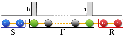
Figure 1: (Color online) The spin graph $\mathcal{K}$ by means of which we aim at achieving high-quality 2-QST via a Rabi-like mechanism between the two ends of the spin chain. The quantum state to be sent is encoded on the spins $\mathcal{S}=\{1,2\}$ (blue), whereas the receivers are located at $\mathcal{R}=\{N-1,N\}$ (red). Barrier qubits, residing at sites $n=\{3,N-2\}$, on which a strong magnetic field $h$ is applied are colored in green.

Eq. (5) can be mapped to a tight-binding spinless fermion model via the Jordan-Wigner transformation LiebSM1961

$$H=-\sum_{i=1}^{N-1}c^{\dagger}_{i}c_{i+1}{+}c_{i}c^{\dagger}_{i+1}{+}h\left(c^{\dagger}_{3}c_{3}{+}c^{\dagger}_{N{-}2}c_{N{-}2}\right),$$ (6)

where we have taken as our energy and inverse time unit the exchange energy $J$, that we consider to be site independent.

Because of the quadratic nature of the Hamiltonian, the single particle spectrum is sufficient to describe the full dynamics. Denoting by $\varepsilon_{k}$ and $\left|\varepsilon_{k}\right>$ the $k$-th energy eigenvalue and its corresponding eigenvector, the full Hamiltonian operator acting on a $2^{N}$ dimensional Hilbert space, is easily decomposed into a direct sum over all particle number-conserving invariant subspaces $H=\bigoplus_{n=1}^{N}H_{n}$, where

$$H_{n}{=}\!\!\!\!\!\!\!\!\sum_{k_{1}{<}k_{2}{<}...{<}k_{n}{=}1}^{N}\!\!\!\!\!\!\!\!\!\!\!\!\left(\varepsilon_{k_{1}}{+}\varepsilon_{k_{2}}{+}...{+}\varepsilon_{k_{n}}\right)c^{\dagger}_{k_{1}}c^{\dagger}_{k_{2}}...c^{\dagger}_{k_{n}}\left|\{0\}\right>\left<\{0\}\right|c_{k_{n}}...c_{k_{2}}c_{k_{1}},$$ (7)

with $\left|\{0\}\right>$ being the fermion vacuum. Each $H_{n}$, therefore can be constructed quite simply once the single-particle spectrum is known. Notice that the specific ordering of the $k_{i}$’s in the sum of Eq. (7) is taken in such a way that unwanted phase factors do not arise when mapping back into spin operators via the inverse Jordan-Wigner transformation.

Therefore, in order to evaluate $\left|\Psi(t)\right>$ as given by Eq. (2), we need the spectral resolution of $H_{1}$, given by the eigenvalues and eigenvectors of the following $N\times N$ tri-diagonal matrix: $T_{ij}=\delta_{i,i+1}{+}\delta_{i,i-1}{+}h_{3,3}{+}h_{N-2,N-2}$, which is easily diagonalizable, at least numerically. Notice that a uniform magnetic field along the $z$-direction has no influence on what follows as it corresponds to adding a term proportional to the Identity in Eq. 6. Hence the eigenvectors do not change, whereas the uniform shift experienced by all of the eigenvalues is cancelled out in the time evolution of the fidelity, which, as we will show below, only depends on energy differences.

Key to our aim is the presence of eigenstates that are at the same time strongly localized on both the sender and the receiver spins. That is, by expanding the Hamiltonian eigenvectors in the position basis $\left|\varepsilon_{k}\right>{=}\sum_{n{=}1}^{N}a_{kn}\left|n\right>$ (where $\left|n\right>\equiv\left|0_{1}....0_{n-1}1_{n}0_{n+1}...0_{N}\right>$ describes a state with a single spin flipped at position $n$), a prerequisite for Rabi-like oscillations based 2-QST protocol to correctly work is that there exists a certain (small) number of eigenstates $\left|\varepsilon_{k}\right>$ for which $a_{kn}$ is non-negligible only for $n=1,2,N{-}1,N$. We find this requirement of edge quadri-localization to be fulfilled for spin chain of lengths $N{\neq}3n{-}1$, where $n\geq 3\in{\mathds{N}}$, when strong magnetic fields are applied on the barrier qubits. The condition $n\geq 3$ is due to the fact that the minimum length of a spin chain allowing for 2 senders, 2 receivers, and 2 barrier qubits is $N\geq 6$.

By writing $H_{1}=\sum_{k=1}^{N}\varepsilon_{k}\left|\varepsilon_{k}\right>\!\!\left<\varepsilon_{k}\right|$ with the eigenvalues taken in increasing order, the localized states are labelled by $k=\{Q[N,3]{-}1,Q[N,3],N{-}Q[N,3]{-}1,N{-}Q[N,3]\}$, where $Q[a,b]$ denotes the quotient. In the following we will refer to these states by $\{q_{i}\}$, $i=1,2,3,4$. In Fig. 2 an instance of such localized structure of the eigenstates is given for $N=46$ and $h=100J$. We observe that there are 4 eigenstates, labelled by $k=14,15,30,31$, that are quadri-localized on the edges, i.e. at sites $n=1,2,45,46$. Besides these four eigenstates, another two are bi-localized on the barrier qubits at sites $n=3,44$; whereas the remaining ones are extended states with negligible amplitudes on the senders, the receivers, and the barriers. As a consequence, the contribution to the dynamics of $\left|\Psi(0)\right>$ of these extended states is negligible up to order $O(h^{-1})$. In the case of $N=3n-1$, on the other hand, two additional extended eigenstates appear, labelled by $k=\{Q[N,3]+1,N-Q[N,3]-2\}$ with a non-negligible value of $a_{kn}$ for $n=1,2,N-1,N$, as shown in Fig. 2 for the case of $N=50$. We will refer to the latter as extended edge-localized states. As a consequence, there are more eigenstates taking part in the time evolution of the initial state and, although, high-quality 2-QST is still attainable, the clear-cut analysis we will give below is, to some extent, complicated by the their presence. Therefore, in the following, we will first consider spin chains of length $N\neq 3n-1$

III.1 Rabi-like 2-QST

Because the quadri-localized states come as a result of the small effective coupling of $\mathcal{S}$ and $\mathcal{R}$ to the quantum channel $\Gamma$ (due to the energy mismatch with the connecting spins at sites $3$ and $N-3$), their energies and eigenstates can be approximated by 1st-order degenerate perturbation theory and read

$$\varepsilon_{q_{i}} = \epsilon^{(0)}_{q_{i}}+\epsilon^{(1)}_{q_{i}},$$

$$\left|\varepsilon_{q_{i}}\right> = \!\!\!\!\!\!\!\!\sum_{n=\{1,2,N-1,N\}}\!\!\!\!\!\!\!\!a_{q_{i}n}\left|n\right>~{},~{}|a_{q_{i}n}|{\simeq}\frac{1}{2},$$ (8)

where $i=1,2,3,4$. Notice that the coefficients of the eigenvectors obey the parity relation $a_{kn}{=}(-1)^{k{+}1}a_{kN{+}1{-}n}$ because of the mirror symmetry of the model BanchiV13 .

Exploiting the quadratic nature of Eq. (6), we can reduce the two-particles transfer amplitude to single-particle ones by means of the relation given in Ref. Wangetal12 ; WangBGS11 ; nPST2

$$g_{nm}^{rs}{=}\begin{vmatrix}f_{n}^{r}&f_{n}^{r{+}1}&\cdots&f_{n}^{s{-}1}&f_{n}^{s}\\ f_{n{+}1}^{r}&\ddots&&&f_{n{+}1}^{s}\\ \vdots&&&&\vdots\\ f_{m}^{r}&\cdots&&&f_{m}^{s}\\ \end{vmatrix}.$$ (9)

Moreover, mirror symmetry BanchiV13 ; mirror implies $|f_{1}^{r}|=|f_{2}^{r{+}1}|$, and perturbation theory allows to retain only the transition amplitudes between the senders and the receivers. Working out all these simplifications the average fidelity given by Eq. (4) reduces to the approximate expression

$$\bar{F_{a}}(t) = \frac{1}{4}+\frac{10}{54}Re\left[f_{1}^{N-1}\right]+\frac{7}{54}Re\left[\left(f_{1}^{N-1}\right)^{2}\right]+\frac{12}{54}|f_{1}^{N-1}|^{2}+\frac{2}{54}|f_{1}^{N}|^{2}$$ (10)

$$+\frac{10}{54}|f_{1}^{N-1}|^{2}Re\left[f_{1}^{N-1}\right]-\frac{10}{54}Re\left[f_{1}^{{N-1}^{*}}f_{1}^{N}f_{2}^{N-1}\right]-\frac{7}{54}Re\left[f_{1}^{N}f_{2}^{N-1}\right],$$

which we remind to be correct up to order $O\left(h^{-1}\right)$.

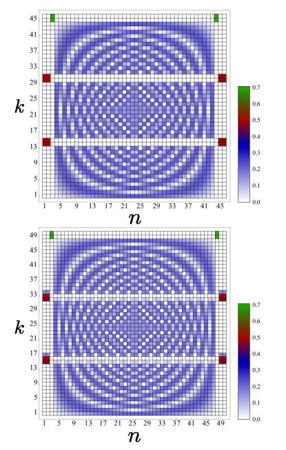
Figure 2: (Color online) Density plot of $|a_{kn}|$ versus $k$ and $n$ for $N=46$ (left) and $N=50$ (right) with $h=100J$. In the case of $N\neq 3n-1$ (left panel) it is clearly shown that the spatial distribution of the eigenvectors exhibits the presence of 4 quadri-localized energy eigenstates; whereas, in the case of $N=3n-1$ (right panel), two more eigenstates appear with non negligible amplitudes also on sites $\mathcal{S}$ and $\mathcal{R}$. Their presence gives rise to a more complicated dynamical behavior of the fidelity because of the larger number of degrees of freedom (and frequencies) effectively entering the time evolution of $\left|\Psi(0)\right>$.

Eq. (10) will be the starting point of the following analysis in which we will evaluate both the maximum achievable fidelity and the optimal transfer time. To start with, let us notice that $\bar{F_{a}}(t)$ only depends on the three complex variables $f_{1}^{N{-}1},f_{1}^{N}$, and $f_{2}^{N{-}1}$, which obey the constraints

$$0 \leq |f_{1}^{N-1}|^{2}+|f_{1}^{N}|^{2}\leq 1,$$

$$0 \leq |f_{1}^{N-1}|^{2}+|f_{2}^{N-1}|^{2}\leq 1,$$ (11)

because of $\sum_{n=1}^{N}|f_{i}^{n}|^{2}=1$, for all $i\in\mathcal{K}$ coming from the conservation of $M^{z}$. Although $f_{1}^{N{-}1}(t),f_{1}^{N}(t)$, and $f_{2}^{N{-}1}(t)$ are complex-valued functions of time, $\bar{F_{a}}(t)$ is a real-valued bounded function, which, taking $\mbox{Re}[f_{s}^{r}(t)]$ and $\mbox{Im}[f_{s}^{r}(t)]$ as independent, becomes a function of six real-valued bounded functions. Therefore, standard Lagrangian multiplier methods can be applied in order to search for the absolute maximum of $\bar{F_{a}}(t)$ within the boundaries given by Eqs. (III.1). It turns out that the maximum of $\bar{F_{a}}(t)$ is given by the conditions $Re[f_{1}^{N-1}(t)]=1$ and $Re[f_{1}^{N}(t)]=Re[f_{2}^{N-1}(t)]=Im[f_{s}^{r}(t)]=0$ (the latter following from the former due to the conservation of $M^{z}$) and amounts to $\bar{F_{a}}(t)=\frac{35}{36}\simeq 0.97$. We found that $\bar{F_{a}}(t)$ does not achieve the maximum possible value of $1$ just because it is an approximate expression for the fidelity: in fact, if the values obtained above for the transition amplitudes are used in the exact expression of the average fidelity given by Eq. (4), we obtain $\bar{F}(t)=1$.

The next step is to find the time $t^{*}$ at which the transition amplitude reaches the optimal values for the 2-QST. To do this, we can maximize the function $Re[f_{1}^{N-1}(t)]$ (or equivalently, due to mirror-symmetry, $Re[f_{2}^{N}(t)]$) whose time evolution is generated by the Hamiltonian given in Eq. (5). This will fix the transfer time $t^{*}$.

Although $\bar{F_{a}}(t)$ is an highly oscillating function because of the presence of many frequencies in the transition amplitudes, it is possible to find the transfer time $t^{*}$ of the 2-QST protocol in a relatively simple way, as we will outline in detail in the following, for the case of even $N{\neq}3n{-}1$.

By exploiting Eqs. (III.1) and by means of elementary trigonometric identities, the term $Re[f_{1}^{N{-}1}]$ can be expressed as

$$Re[f_{1}^{N{-}1}] = Re[\sum_{k{=}1}^{N}e^{-i\varepsilon_{k}t}a_{k1}a_{kN{-}1}]$$ (12)

$$\simeq Re[\sum_{i{=}1}^{4}e^{-i\varepsilon_{q_{i}}t}a_{q_{i}1}a_{q_{i}N{-}1}],$$

which, for even $N$, becomes

$$Re[f_{1}^{N-1}] \simeq (-1)^{Mod[N,3]{+}1}\times$$ (13)

$$\times\left(\sin\omega_{0}^{-}t\cos\omega_{0}^{+}t\sin\omega_{1}^{-}t\cos\omega_{1}^{+}t\right.+$$

$$\left.+\cos\omega_{0}^{-}t\sin\omega_{0}^{+}t\cos\omega_{1}^{-}t\sin\omega_{1}^{+}t\right),$$

where

$$\omega_{0}^{\pm} = \left|\frac{\omega^{\pm}_{14}+\omega^{\pm}_{23}}{2}\right|,$$

$$\omega_{1}^{\pm} = \left|\frac{\omega^{\pm}_{14}-\omega^{\pm}_{23}}{2}\right|,$$

$$\omega_{ij}^{\pm} = \frac{\varepsilon_{q_{i}}\pm\varepsilon_{q_{j}}}{2},$$ (14)

and $Mod[a,b]$ is the modulus function.

Having defined in such a way the frequencies that enter the dynamics of $Re[f_{1}^{N{-}1}]$, it turns out that $\omega_{0}^{-}{\gg}\omega_{0}^{+}{\gg}\omega_{1}^{-}{\gg}\omega_{1}^{+}$, which immediately sets a time scale for the 2-QST. In fact, as $\omega_{1}^{+}t{\ll}1$, we can focus only on the first summand of the RHS in Eq. 13, namely $\sin\omega_{0}^{-}t\cos\omega_{0}^{+}t\sin\omega_{1}^{-}t$. On the same footing, the next time scale is given by $\omega_{1}^{-}$, which implies that the maximum of $Re[f_{1}^{N{-}1}](t)$ has to be found in the neighborhood of $t_{1}{=}\frac{\pi}{2\omega_{1}^{-}}$, which, hence, approximately gives the optimal time $t^{*}$. As a result, the transfer time $t^{*}$ is found by solving

$$t^{*}=\begin{cases}\max\left[\sin\omega_{0}^{-}t\cos\omega_{0}^{+}t\right]&~{}~{}\mbox{if }\,Mod[N,3]\mbox{ is }\,\textit{odd}\\ \min\left[\sin\omega_{0}^{-}t\cos\omega_{0}^{+}t\right]&~{}~{}\mbox{if }\,Mod[N,3]\mbox{ is }\,\textit{even}\end{cases}$$ (15)

and by choosing the solution closest to the time $t_{1}$. A graphical representation of these timescales is given in Fig. 3, which also allows us to put forward a simple physical interpretation. In fact, from the left panel of Fig. 3, $\sin\omega_{1}^{-}t$ can be seen as an approximate envelope for the fidelity of the transfer process, whereas $\omega_{0}^{-}\simeq 2J$ gives the time-scale for the (very rapid) bouncing of the excitation back and forth between the two receivers. These oscillations occur because of the direct coupling between the two receiver spins and could be eliminated if this coupling is switched off.

This bouncing occurs many times (see the right panel of Fig. 3) before the excitation slowly leaves these two sites to go back towards the senders. In Fig. 4 we compare the approximate value of the fidelity given by Eq. (10) with the exact result of Eq. (4): it is shown that $\bar{F}(t){>}\bar{F}_{a}(t)$ attaining values as high as 0.999. We checked, up to computational accessibility, that this holds true for every $N$.

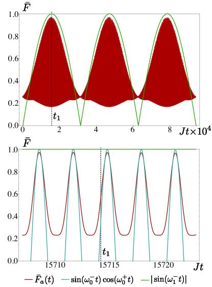
Figure 3: (Color online) (left) Approximated average fidelity $\bar{F}_{a}(t)$, and, for comparison, $\left|\sin\omega_{1}^{-}t\right|$ shown as a function of time. Notice that $F_{a}$ is so rapidly oscillating that it appears to fill the entire red region in the plot. The sinusoidal function approximately gives an envelop of the fidelity with the same periodicity, which easily allows us to identify several reading windows for the 2-QST. (right) Full expression for the average fidelity $\bar{F}_{a}(t)$ (red), $\sin\omega_{0}^{-}t\cos\omega_{0}^{+}t$ (blue) and $\sin\omega_{1}^{-}t$ (green) shown as a function of time around the optimal transfer time $t_{1}$, denoted by the vertical dashed line. Notice that $|\sin\omega_{1}^{-}t|\simeq 1$ and that the fidelity attains very high values near $t_{1}$ which recur several times, with a frequency of order of $J^{-1}$, allowing again for several reading windows.

The Rabi-like half-oscillation time $t_{1}$, giving an approximate value of the optimal time for the excitation transfer from $\mathcal{S}$ to $\mathcal{R}$, can be obtained by using standard degenerate time-independent perturbation theory to evaluate the relevant energy eigenvalues. Here we report the energy corrections for the dynamically relevant states given in Eq. (III.1) up to the first order in $h^{-1}$. Denoting by $x_{i}$, with $x_{1}{>}x_{2}{>}x_{3}$, the solutions of ${-}x^{3}{-}hx^{2}{+}2x{+}h{=}0$, and defining the parameters $\beta_{1,2}=h{+}x_{1,2}$, $\alpha=x_{1,2}^{2}{+}hx_{1,2}{-}1$, and $\gamma=\left(2\left(\alpha_{1,2}^{2}{+}\beta_{1,2}^{2}{+}1\right)\right)^{-\frac{1}{2}}$, we obtain

$$\varepsilon_{q_{1}}=\lambda_{1}^{-}~{},~{}\varepsilon_{q_{2}}=\lambda_{1}^{+}~{},~{}\varepsilon_{q_{3}}=\lambda_{2}^{+}~{},~{}\varepsilon_{q_{4}}=\lambda_{2}^{-}~{},$$ (16)

where

$$\lambda_{1,2}^{\pm}=2\left(z_{1,2}+\frac{\gamma_{1,2}^{2}}{N-5}\sum_{k=1}^{N-6}\frac{\left(\left(1\pm\cos k\pi\right)\sin\frac{k\pi}{N-5}\right)^{2}}{z_{1,2}+2\cos\frac{k\pi}{N-5}}\right).$$ (17)

Finally, using Eqs. (III.1) and (16), we obtain the approximate transfer time $t_{1}{\simeq}/\left[2\left(\lambda^{-}_{1}{-}\lambda^{+}_{1}{+}\lambda^{-}_{2}{-}\lambda^{+}_{2}\right)\right]$. We also find that $t_{1}$ scales quadratically with the magnetic field intensity and that it is independent of $N$, $t_{1}{=}\frac{\pi}{2}h^{2}{+}(-1)^{Mod[N,3]}\frac{Mod[N,2]\pi}{2}h$, as reported in Fig. 4 for the case of $N{=}30$. Notice that in 1-QST schemes in which the magnetic field is applied directly on the sender and the receiver, the transfer time scales exponentially both with the length of the chain $N$ and with the magnetic field’s intensity $h$ Rabi-like3 ; Rabi-like5 .

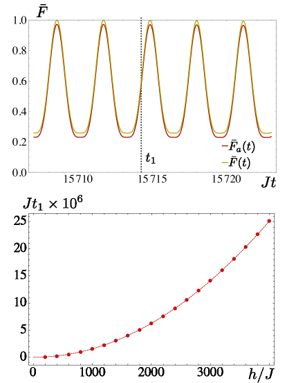
Figure 4: (Color online) (left) Exact average fidelity $\bar{F}(t)$ (yellow) and approximate fidelity $\bar{F}_{a}(t)$ (red) versus $t$ around $t_{1}$. Notice that $\bar{F}(t)>\bar{F}_{a}(t)$ is always fulfilled and that, at the optimal time $t^{*}$ almost perfect quantum state transfer is achieved, with $\bar{F}(t)\simeq 0.999$. (right) Transfer time $t^{*}$ versus $h$ for $N=30$: the function $f(h)=\frac{\pi}{2}h^{2}$ (dashed line) fits perfectly with the numerical data for $t^{*}$. The range of values of the magnetic field $h$ is such that $\bar{F}_{a}(t)>0.95$.

A similar procedure for odd $N{\neq}3n-1$ yields for the transfer amplitude of Eq. (12)

$$Re[f_{1}^{N-1}] \simeq (-1)^{Mod[N,3]}\times$$ (18)

$$\times\left(\cos\omega_{0}^{-}t\sin\omega_{0}^{+}t\sin\omega_{1}^{-}t\cos\omega_{1}^{+}t\right.$$

$$\left.+\sin\omega_{0}^{-}t\cos\omega_{0}^{+}t\cos\omega_{1}^{-}t\sin\omega_{1}^{+}t\right),$$

and the optimal transfer time $t^{*}$ can be found via a double step, with a recipe similar to the one discussed above. First we determine $t_{2}$, defined as the solution of $\sin\omega_{0}^{+}t{=}(-1)^{Mod[N,3]}$ which is closest to $t_{1}{=}\frac{\pi}{2\omega_{1}^{-}}$, and then $t^{*}$ is given by the solution of $\cos\omega_{0}^{-}t{=}1$ which is closest to $t_{2}$. Notice that this is not different from the previous procedure; indeed, there are many ways to recast Eq. (12) by combining the energies $\varepsilon_{q_{i}}$, and the fact that we obtained an apparently different method for $t^{*}$ in the Eqs. (13) and (18), for even and odd $N$, respectively, is due to the fact that we kept unchanged the definitions of the frequencies given by Eq. (III.1) to avoid a confusing re-labelling.

III.2 Quasi Rabi-like 2-QST

Let us now go back to the case of spin chains of length $N{=}3n{-}1$, that was left out of the previous analysis. In this case, two additional edge-localized extended states are found, whose presence hinders the clear Rabi-like oscillations of the excitation between $\mathcal{S}$ and $\mathcal{R}$, exhibited in the case of $N{\neq}3n{-}1$ by the sinusoidal function $\sin\omega_{1}^{-}t$ and reported in the previous subsection and in Fig. 3. Nevertheless, since the number of eigenstates (eigenenergies) to be included in the sum given in Eq. 12 increases just by two, an analysis similar to the one performed above can still be carried out. We dub the transmission process in this case as quasi Rabi-like 2-QST.

In fact, the approximated expression for $Re[f_{1}^{N-1}(t)]$ given in Eq. (12) now becomes

$$Re[f_{1}^{N{-}1}] \simeq Re[\sum_{i{=}1}^{6}e^{-i\varepsilon_{q_{i}}t}a_{q_{i}1}a_{q_{i}N{-}1}]=$$ (19)

$$= \pm 2\left(c_{1}\cos\omega_{14}^{+}t\cos\omega_{14}^{-}t+\right.$$

$$-c_{2}\cos\omega_{25}^{+}t\cos\omega_{25}^{-}t+$$

$$+\left.c_{3}\cos\omega_{36}^{+}t\cos\omega_{36}^{-}t\right),$$

with the $\pm$ sign holding for even (odd) $N$, respectively, and where we exploited the mirror-symmetry and used $1$st-order degenerate perturbation theory relations

$$c_{1} = a_{11}a_{1N-1}\simeq a_{41}a_{4N-1}\simeq\frac{1}{4}-\frac{3}{2N-1},$$ (20)

$$c_{2} = a_{21}a_{2N-1}\simeq a_{51}a_{5N-1}\simeq\frac{1}{4},$$ (21)

$$c_{3} = a_{31}a_{3N-1}\simeq a_{61}a_{6N-1}\simeq\frac{3}{2N-1}.$$ (22)

Using the approximations $\omega_{14}^{-}\simeq\omega_{25}^{-}\simeq\omega_{36}^{-}\simeq-2$ and $\omega_{36}^{+}\simeq 0$, yields

$$Re[f_{1}^{N{-}1}]\simeq\pm\cos 2t\left(4c_{3}\sin\omega_{14}^{+}t-\sin^{2}\omega_{14}^{+}t\right).$$ (23)

Once again, it is possible to identify two different processes: the slow quasi-Rabi-like oscillations of the excitation between $\mathcal{S}$ and $\mathcal{R}$, having a time scale ruled by $\omega_{14}^{+}$, and the fast oscillations of the excitation within $\mathcal{R}$ ($\mathcal{S}$) triggered by $J$ and described by the term $\cos 2t$. Although the additional states complicate somehow the expression of $Re[f_{1}^{N{-}1}]$, they also provide a clear advantage as far as the transfer time is concerned. Indeed the time $t_{1}$ is now linear in the magnetic field and hence 2-QST occurs faster w.r.t. chains of length $N{\neq}3n{-}1$. Let us remind that a similar phenomenon takes place in 1-QST protocols where the sender and the receiver are weakly coupled to the chain either because of smaller bond strengths Rabi-like4 or because of a strong magnetic field acting on barrier qubits Rabi-like6 . Indeed, in those cases the QST time for even- and odd-length chains too scales, respectively, quadratically and linearly with the perturbation’s intensity.

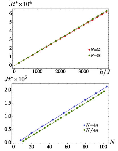
Figure 5: (Color online) (left) Transfer time $t^{*}$ for the case of spin chain’s of length $N{=}3n{-}1$ as a function of $h$. The time $t^{*}$ increases linearly with $h$, although with slightly different coefficients depending on wether $N$ is divisible by $4$ or not. In the figure the two cases are exemplified by $N{=}32$ and $N{=}38$, respectively. (right) Transfer time $t^{*}$ for the case of spin chain’s of length $N{=}3n{-}1$ with magnetic field $h{=}4000$ as a function of $N$. The time increases linearly with $N$, with clearly distinct coefficients depending on the divisibility by 4 of $N$.

In Fig. 6, we summarize the main result of the two previous subsections, namely the possibility to transfer with high-fidelity an arbitrary quantum state of two qubits by means of a linear spin-$\frac{1}{2}$ chain with strong magnetic fields on the barrier qubits. It is shown that for $N{\neq}3n{-}1$, a fidelity close to unity can be achieved regardless of $N$ (provided strong enough magnetic fields are applied at the barrier sites) although in a time that increases quadratically with $h$. For $N{=}3n{-}1$, instead, the quality of the transfer depends on whether $N$ is divisible by 4 (higher $\bar{F}_{a}(t^{*})$) or not (lower $\bar{F}_{a}(t^{*})$), but the transfer is achieved in a time that scales only linearly with both $h$ and $N$. Nevertheless, the differences amongst all these cases fade away for $N{\gg}1$, where all curves collapse.

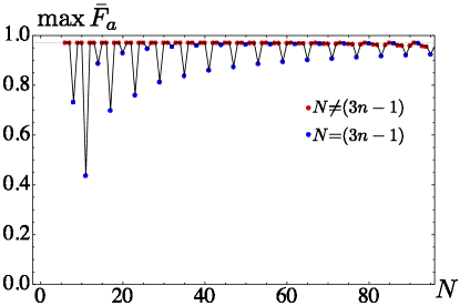
Figure 6: (Color online) Maximum of the approximate fidelity $\bar{F}_{a}(t^{*})$ obtained by choosing $h{=}4000$. The red points are the Rabi-like 2-QST and the maximum does not depend on $N$, the blue point are for $N{=}3n{-}1$ and even $N$ performs better than odd $N$. For $N{\gg}1$, both of the curves converge to the $N{\neq}3n{-}1$ case.

Since the average fidelity is not identically one, one could imagine that there exist specific input states that are transferred with a relatively poor quality. This is not the case, and in order to dispel such a doubt, we evaluated also the worst case fidelity ballistic1 and found that the minimum state-dependent fidelity, evaluated by means of Eq. 3, remains close to the average one up to the fourth digit, i.e. $F_{min}\simeq 0.999$.

To conclude this Section we stress that the probability to find the excitations inside the quantum channel $\Gamma$, evaluated by $\sum_{n=3}^{N-2}\left(\left|f_{1}^{n}(t)\right|^{2}+\left|f_{2}^{n}(t)\right|^{2}\right)$, is radically different depending on whether $N{\neq}3n{-}1$ or not. In the former case it is of the order of $O(h^{-1})$ because $\Gamma$ acts as a mere physical connector Rabi-like3 ; Rabi-like4 ; Rabi-like9 entering the dynamics only virtually. On the contrary, when $N{=}3n{-}1$, two extended states with a non-negligible overlap on the senders and the receivers come into play, meaning that the excitations can be actually found inside the channel $\Gamma$. As a consequence, the effect of a dissipative coupling of an environment eventually acting only on $\Gamma$ has a negligible influence only for the Rabi-like QST whereas for the quasi-Rabi-like one the quality could be severely degraded, especially for short chains. For long chains, on the other hand, since the overlap with the extended state localized also on the edges scales as $c_{3}\sim O(N^{-1})$, the degrading effect becomes negligible. On the other hand, the presence of disorder in the couplings or in a magnetic field acting on the quantum channel $\Gamma$ should have a negligible influence too on the efficiency of the 2-QST protocol we are proposing here, regardless of $N$, as long as the spatial distribution of the eigenvectors depicted in Fig. 2 is not significantly affected disorder1 ; disorder2 ; disorder3 .

IV Conclusions

In this paper, we derived an expression for the average fidelity of the quantum state transfer of two qubits through a spin-$\frac{1}{2}$ chain, providing that the $z$-total angular momentum is conserved and all the spins are initially aligned. This general expression, relating the average fidelity explicitly to one- and two-particle transition amplitudes, may result useful in investigating the two qubit QST properties of a wide range of physical models displaying the above-mentioned characteristics.

Furthermore, we discussed a specific case, obtained by extending a Rabi-like protocol, widely adopted for QST of single qubits, to the non-trivial case of the QST of two qubits, where the senders and receivers pairs are located at each end of a one dimensional spin-$\frac{1}{2}$ chain with $XX$-Heisenberg type nearest-neighbor interactions. The presence of strong magnetic fields on the two sites closest to the sender and receiver (barrier qubits), allowed us to obtain a faithfully transfer for an arbitrary two-qubits quantum state. We characterized the quality of the 2-QST by using first-order degenerate perturbation theory; thus providing, apart from a clear-cut physical interpretation of the multi-excitation dynamics yielding high-quality 2-QST, also an approximate analytical expression for the time transfer. The latter is found to increase linearly or quadratically with the magnetic field intensity $h$ depending on the spin chain length. Moreover, we have verified that the worst-case fidelity of the QST remains almost unchanged with respect to the average one, i.e., $\simeq 0.999$.

Two final comments are in order. Since it is straightforward that the 4-dimensional Hilbert space of the senders can be also employed to encode an $n<4$ qudit to be transferred to the receivers, the scheme we propose can be adapted to the transfer of qutrits (qubits) encoded in arbitrary three (two) orthogonal quantum states of the senders. Finally, the question if the barrier scheme discussed here is useful in order to perform QST of an arbitrary number of qubits will be left to future investigations.

V Acknowledgement

TJGA and GMP acknowledge the EU Collaborative Project TherMiQ (Grant Agreement 618074). SL and GMP acknowledge support by MIUR under PRIN 2010/11 TJGA thanks the International Institute of Physics - UFRN (Natal, Brazil) for the kind hospitality provided during part of this work. SP is supported by a Rita Levi-Montalcini fellowship of MIUR. SP and TJGA acknowledge partial support from MCTI and UFRN/MEC (Brazil).

References

- (1) W. K. Wootters , W. H. Zurek, Nature 299, 802 (1982).
- (2) S. Bose, Phys. Rev. Lett. 91, 207901 (2003).
- (3) S. Bose, Contemp. Phys. 48, 13 (2007).
- (4) T.J.G. Apollaro, S. Lorenzo, F. Plastina, Int. J. Mod. Phys. B 27, 1345035 (2013).
- (5) Y. Liu, D. L. Zhou, New J. Phys. 17, 013032 (2015).
- (6) C. Di Franco, M. Paternostro, M. S. Kim, Phys. Rev. A 81, 022319 (2010).
- (7) C. M. Rafiee, H. Mokhtari, Eur. Phys. J. D 66, 269 (2012).
- (8) M. Christandl, N. Datta, A. Ekert,A. J. Landahl, Phys. Rev. Lett. 92, 187902 (2004 ).
- (9) C. Di Franco, M. Paternostro and M. S. Kim, Phys. Rev. Lett. 101, 230502 (2008).
- (10) A. Casaccino, S. Lloyd, S. Mancini, S. Severini, Int. J. Quantum. Inf. 7, 1417 (2009).
- (11) S. Paganelli, G. L. Giorgi, F. de Pasquale, Fortschr. Phys. 57, 1094 (2009).
- (12) L. Banchi et al., Phys. Rev. A 82, 052321 (2010).
- (13) A. Zwick, O. Osenda, J. Phys. A:Math. Theor. 44, 105302 (2011).
- (14) L. Banchi et al., New J. Phys. 13, 123006 (2011).
- (15) T. J. G. Apollaro et al., Phys. Rev. A 85, 052319 (2012).
- (16) L. Banchi, Eur. Phys. J. Plus 128 137, (2013).
- (17) T. J. G. Apollaro, F. Plastina, Phys. Rev. A 74, 062316 (2006).
- (18) S. Paganelli, F. de Pasquale, G. L. Giorgi, Phys. Rev. A 74, 012316 (2006).
- (19) F. Plastina and T. J. G. Apollaro, Phys. Rev. Lett. 99, 177210 (2007).
- (20) M. Markiewicz, M. Wiesniak, Phys. Rev. A 79, 054304 (2009).
- (21) N. Y. Yao et al, Phys. Rev. Lett. 106, 040505 (2011).
- (22) T. Linneweber, J. Stolze and G. S. Uhrig, Int. J. Quantum Inform. 10, 1250029 (2012 ).
- (23) S. Lorenzo, T. J. G. Apollaro, A. Sindona and F. Plastina, Phys. Rev. A 87, 042313 (2013).
- (24) G. L. Giorgi and T. Busch, Phys. Rev. A 88, 062309 (2013).
- (25) B. Chen, Y. Li, Z. Song and C. P. Sun, Ann. Physics 348, 278 (2014).
- (26) K. Korzekwa, P. Machnikowski, P. Horodecki, Phys. Rev. A 89, 062301 ( 2014).
- (27) F. de Pasquale, G. L. Giorgi and S. Paganelli, Phys. Rev. A 71, 042304 (2005).
- (28) F. de Pasquale, G. L. Giorgi and S. Paganelli, Phys. Rev. Lett. 93, 120502 (2004).
- (29) A. Bayat, S. Bose, P. Sodano, Phys. Rev. Lett. 105, 187204 (2012).
- (30) S. Paganelli, S. Lorenzo, T. J. G. Apollaro F. Plastina, G. L. Giorgi Phys. Rev. A 87, 062309 (2013).
- (31) N. Behzadi, S. K. Rudsary, B. A. Salmasi, Eur. Phys. J. D 67, 252 (2013).
- (32) D. Burgarth, V. Giovannetti, S. Bose, J. Phys. A 38, 6793 (2005).
- (33) M. Christandl et al, Phys. Rev. A 71, 032312 (2005).
- (34) A. Bayat Phys. Rev. A 89, 062302 (2014).
- (35) A. Kay Int. J. Quantum Inform. 8, 641 (2010).
- (36) R. Sousa, Y. Omar, New J. Phys. 16, 123003 (2014).
- (37) P. Lorenz, J. Stolze, Phys. Rev. A 90, 044301 (2014).
- (38) M. A. Nielsen and I. L. Chuang, Quantum Computation and Quantum Information, Cambridge University Press (2000) ; V. Vedral Introduction to Quantum Information Science, Oxford University Press (2007).
- (39) R. Jozsa, J. Mod. Opt. 41, 2315 (1994).
- (40) T. J. G. Apollaro, S. Lorenzo, A. Sindona, S. Paganelli, G. L. Giorgi, F. Plastina, arXiv:1404.7837, (2014).
- (41) M. Horodecki, P. Horodecki, R. Horodecki Phys. Rev. A 60, 1888 (1999).
- (42) V. Buz̆ek, M. Hillery, Phys. Rev. Lett. 81, 5003 (1998).
- (43) E. Lieb, T. Schultz, D. Mattis, Ann. Physics 16, 407 (1961).
- (44) L. Banchi, R. Vaia, J. Math. Phys. 54, 043501 (2013).
- (45) Z-M Wang , C. A. Bishop , Y-J Gu , B. Shao, Phys. Rev. A 84, 022345 (2011).
- (46) Z-M Wang et al., Phys. Rev. A 86, 022330 (2012).
- (47) P. Karbach, J. Stolze, Phys. Rev. A 72, 030301(R) (2005).
- (48) A. Zwick et al., Phys. Rev. A 85, 012318 (2012).
- (49) A. Zwick et al., Phys. Rev. A 84, 022311 (2011) .
- (50) A. Zwick, G. A. Alvarez, G. Bensky, G. Kurizki, New J. Phys. 16, 065021 (2014).