Controlling disorder with periodically modulated interactions

Abstract

We investigate a celebrated problem of the one dimensional tight binding model in the presence of disorder leading to Anderson localization from a novel perspective. A binary disorder is assumed to be created by immobile, heavy particles that affect the motion of the lighter, mobile species in the limit of no interaction between mobile particles. Fast, periodic modulations of interspecies interactions allow us to produce an effective model with small diagonal and large off-diagonal disorder previously unexplored in cold atom experiments. We present an expression for an approximate Anderson localization length and verify the existence of the well known, extended resonant mode. We also analyze the influence of nonzero next-nearest neighbor hopping terms. We point out that periodic modulation of interaction allows disorder to work as a tunable band-pass filter for momenta.

I Introduction

Anderson localization (AL) in disordered systems has fascinated and stimulated physicists for more than 50 years Anderson (1958); Lagendijk et al. (2009). For one-dimensional (1D) systems, as discussed below, a particle propagating with momentum $k$, in a disordered medium, undergoes multiple scatterings and eventually localizes with an exponentially decaying density profile Mott and Twose (1961); Lee and Ramakrishnan (1985); Ishii (1973). The AL is a single-particle interference effect which cannot be observed directly in solid-state systems due to the presence of electron-electron and electron-phonon interactions. AL has been widely studied for various systems including tight binding models with diagonal disorder and nearest-neighbor (nn) and/or next-nearest-neighbor (nnn) hopping Biddle et al. (2011); Sepehrinia (2010); Eilmes et al. (1998); Yamada (2004).

Ultracold atomic gases have become a playground where complex systems can be simulated and investigated Bloch et al. (2008); Jaksch and Zoller (2005); Lewenstein et al. (2012). In particular, optical lattice engineering allows a high degree of controllability. Various techniques, i.e. periodic modulation of lattice positions and amplitudes Eckardt et al. (2005); Lignier et al. (2007); Struck et al. (2011) or Feshbach resonance Chin et al. (2010), are used to effectively tune parameters of a given model Struck et al. (2012); Windpassinger and Sengstock (2013); Sacha et al. (2012); Eckardt et al. (2010); Przysiężna et al. (2015). The level of experimental control and detection allows one to build quantum simulators, i.e., experimentally controlled systems that are able to mimic other systems difficult to investigate directly Buluta and Nori (2009); Hauke et al. (2012). Ultracold atomic gases are ideal systems for theoretical and experimental investigation of the Anderson localization of matter waves. An experimental observation of AL was first realized in one dimension seven years ago Billy et al. (2008) (a closely related Aubry-André Aubry and André (1980) localization was also realized Roati et al. (2008) independently. For reviews see Aspect and Inguscio (2009); Modugno (2010). Recently AL was observed also in three dimensions Jendrzejewski et al. (2012); Kondov et al. (2011) in speckle potentials. In all these experiments, in order to get rid of particle interactions, either Feshbach resonances Chin et al. (2010) were employed or a low atomic density limit was reached.

Typically in cold atom disorder experiments, as well as theoretical propositions, the disorder appears in a diagonal form, either on the chemical potential level (lattice site energies) like for quasi-periodic lattices Roati et al. (2008) or for interactions Gimperlein et al. (2012). Similarly, a diagonal disorder appears for a binary disorder that is introduced by interactions with other species Gavish and Castin (2005); Massignan and Castin (2006); Ospelkaus et al. (2006); Horstmann et al. (2007a); Krutitsky et al. (2008). On the other hand, a more detailed analysis shows that for cold atoms the off-diagonal disorder, i.e. a disorder in tunnelings, appears in quite a natural way both for the incommensurate superlattice potential roscilde and for the speckle random potential perturbing the optical lattice Semmler et al. (2010). However in both these cases, the disorder in tunneling is strongly correlated with the diagonal disorder. The aim of this paper is to show that periodic modulations of interactions allow a transfer of the disorder to the kinetic energy (tunneling terms) creating a tunable off-diagonal disorder opening up the possibility of its study in controllable cold atoms settings.

The interest in off-diagonal disorder stems from the fact that it can profoundly affect the properties of the system. Consider, for example, the case when the disorder is purely off-diagonal. There has been a long debate about the nature of states in the center of the band. The first works bush75 ; Theodorou76 ; Antoniou77 showed that the localization length diverges in the center of the energy band (i.e. $E=0$), therefore it was argued that a transparency window appears and even the one-dimensional system exhibits the mobility edge. However, in the early eighties it has been established that even for a purely off-diagonal disorder all states are localized Soukoulis81 ; Pendry (1982); Delyon83 ; Krey (1983). The puzzle of the $E=0$ state was solved showing that the wavefunction envelope scales as $exp(-\gamma\sqrt{N})$ with $N$ being the system size Soukoulis81 . In the presence of both diagonal and off-diagonal disorder all states remain localized Bovier89 except very special cases of correlated diagonal and off-diagonal disorder Flores (1989). Additional details, especially in the context of conductance anomalies, may be found in Alloatti09 .

Possible correlations in the system and/or in the disorder may also profoundly affect localization properties Dunlap et al. (1990); deMoura98 ; Piraud et al. (2013). A famous example is the dimer model Dunlap et al. (1990) in which sites may have energies $\epsilon_{a}$ and $\epsilon_{b}$ with the constrain that $\epsilon_{b}$-sites come only in pairs. This short-range correlation leads to delocalized states. A similar situation occurs for the dual random dimer model (DRDM) in which consecutive sites may not have $\epsilon_{b}$ energy. The model has several applications in different areas from DNA studies Caetano ; Zhang et al. (2010) to photonic systems Zhao . The cold atom version of DRDM has been proposed by Schaff, Akdeniz, and Vignolo Schaff et al. (2010) who have shown that by tuning the interaction between atomic species one may observe the localization-delocalization transition and study the extended resonant mode. In our proposition we modify the approach proposed in Schaff et al. (2010) by periodically modulating the interactions which allows us a great freedom in changing the relative importance of diagonal and off-diagonal disorder in the system. For such a model we calculate the approximate Anderson localization length and compare it with numerical results. We show that the delocalization window may serve as a narrow energy filter for the particles. In addition we point out that the extended mode is vulnerable to effects due to next-nearest neighbor tunneling limiting its existence to relatively deep lattices. Details of numerical methods needed to calculate the Anderson localization length with next-nearest neighbor random tunneling are presented in the Appendix B.

II The model

We consider a simple, standard one-dimensional non-interacting tight-binding Hamiltonian (with $\hbar=1$)

$$H=\sum_{i}\left(\epsilon_{i}n_{i}-J(a^{\dagger}_{i}a_{i+1}+\mathrm{h.c.})\right),$$ (1)

where $a_{i}$ ($a^{\dagger}_{i}$) denotes an annihilation (creation) operator of bosons at site $i$, $n_{i}=a^{\dagger}_{i}a_{i}$ is a particle counting operator, $\epsilon_{i}$ are on-site energies while $J$ is the tunneling amplitude which will serve as our energy scale. Let us apply a periodic modulation of the on-site energies

$$\epsilon_{i}\to\epsilon_{i}(1+\delta\sin(\omega t)),$$ (2)

where $\delta$ is the modulation amplitude and $\omega$ its frequency.

Hamiltonian (1) has periodic time dependence $H(t)=H(t+2\pi/\omega)$. In such a case we can use the well established formalism of Floquet theory Floquet (see also Shirley ) extensively used, in the last century, to study the influence of optical or microwave fields on atoms. Recently it has been applied with great success for controlling properties of ultra-cold atomic systems Eckardt et al. (2005); Lignier et al. (2007); Struck et al. (2011). Solutions of equation $i\partial_{t}|\psi_{n}(t)\rangle=H(t)|\psi_{n}(t)\rangle$ have a form of Floquet states: $|\psi_{n}(t)\rangle=e^{-i\varepsilon_{n}t}|u_{n}(t)\rangle$, where $\varepsilon_{n}$ is called the quasienergy and $|u_{n}(t)\rangle$ have periodicity of the Hamiltonian. The Floquet theorem is a time analogue of the Bloch theorem for spatially periodic potentials. Although we can not treat $|\psi(t)\rangle$ as eigenstates of $H(t)$, $|u(t)\rangle$ are eigenstates of the Floquet Hamiltonian $\mathcal{H}(t)=H(t)-i\partial_{t}$ existing in the extended space of $T$-periodic functions. In that space we can number states using a new quantum number $m\in\mathbb{Z}$: $|u^{m}_{n}\rangle=|u_{n}\rangle e^{i\omega mt}$, where $|u_{n}^{m}\rangle$ is the eigenstate to the eigenenergy $\varepsilon^{m}_{n}=\varepsilon_{n}+\omega m$. This whole class corresponds to one physical state $|\psi_{n}(t)\rangle$ as adding $\omega$ to $\varepsilon_{n}$ in physical space only takes us to the next “Brillouin zone” for quasienergies. Therefore, it is sufficient to find a block-diagonal form of a Hamiltonian (in $m$-ordered basis) and consider only one block corresponding to a single “Brillouin zone”. Unfortunately, couplings between different blocks make the block-diagonalization a formidable task. One may, however, make a unitary transformation $U$:

$$\mathcal{H}^{\prime}=U\mathcal{H}U^{\dagger},\quad U=\exp{\left[-i\delta\frac{\cos(\omega t)}{\omega}\sum_{i}\epsilon_{i}n_{i}\right]},$$ (3)

$$\mathcal{H}^{\prime}(t)=\sum_{i}\left(\epsilon_{i}n_{i}-(e^{i(\epsilon_{i+1}-\epsilon_{i})\frac{\delta\cos(\omega t)}{\omega}}a^{\dagger}_{i}a_{i+1}+\mathrm{h.c.})\right).$$ (4)

In effect, for frequencies $\omega\gg 1$ (in units of $J$) one we can neglect the couplings between different Floquet blocks and consider only one diagonal block governing the long term ($t\gg 1/\omega$) dynamics:

$$H_{\mathrm{eff}}=\frac{1}{T}\int_{0}^{\frac{2\pi}{\omega}}dt\mathcal{H}^{\prime}(t)=\sum_{i}\left(\epsilon_{i}n_{i}-(t_{i}a^{\dagger}_{i}a_{i+1}+\mathrm{h.c.})\right),$$ (5)

where

$$t_{i}=\mathcal{J}_{0}\left(\frac{\delta}{\omega}(\epsilon_{i+1}-\epsilon_{i})\right)$$ (6)

is the effective position dependent hopping and $\mathcal{J}_{0}$ is the zero-th order Bessel function. It has been verified experimentally Lignier et al. (2007); Struck et al. (2011) that the effective time-averaged Hamiltonian governs the dynamics of periodically driven systems for long times. In particular, localization properties of eigenstates of (5) will be shared by the Floquet eigenstates of the original Hamiltonian (1) [with the fast modulation (2)] after averaging them over the period. This may be understood by inspecting the unitary operator $U$ in (3) and observing that it consists of a product of local operators acting on single sites. Thus $U$ adds only local phases to single particle states – that cannot affect the resulting density distribution. Further detailed discussion of the construction of the effective Hamiltonians for high frequency periodically driven systems may be found in rahav03 ; eckardt15 ; bukov15 .

Note that for a uniform system with all $\epsilon_{i}$ being the same, the tunneling, (6) is unaffected, while $t_{i}$ changes if on-site energies vary from site to site. Such is the case for superlattices Esmann et al. (2011); Di Liberto et al. (2014) or external potentials such as a harmonic trap or a linear tilt Eckardt et al. (2005). In this work we will consider the on-site energy variations due to disorder.

It is worth noting that it is usually possible to adiabatically pass from eigenstates of one $H_{\mathrm{eff}}$ to another (e.g. for different $\delta$) if the change of parameters is slow enough Poletti and Kollath (2011). Thus it is possible to prepare a time independent system and turn on periodic modulation, or change modulation parameters during experiments. For completeness let us note that, for the tight-binding description in terms of a single lowest band to be valid in (1-5), $\omega$, while much larger than the tunneling amplitude, must be smaller than the energy separation to the excited band Eckardt et al. (2005); lacki2013 .

To create disorder we consider two species of atoms repulsively interacting with each other but allow only one of them to move freely on the lattice. The frozen atoms (denoted with a superscript $f$) give rise to a binary disorder Gavish and Castin (2005); Horstmann et al. (2007a); Horstmann et al. (2010); Ospelkaus et al. (2006). The mobile particles are assumed not to interact among themselves. They can be spin-polarized fermions or bosons with interactions tuned off by microwave or optical Feshbach resonance Chin et al. (2010). The dynamics of the system can be described by a single particle Hamiltonian with the on-site energy $\epsilon_{i}=Vn^{f}_{i},$ where $V$ denotes an interspecies contact interaction. When frozen particles are fermions or strongly repelling (hard-core) bosons their occupation per lattice site $n^{f}_{i}$ takes either a value of zero or one and the on-site energy takes only two values $\epsilon_{i}\in\{0,V\}$. Further, we consider the particular case of DRDM when two adjacent sites cannot be occupied by frozen atoms simultaneously Dunlap et al. (1990). For cold atoms DRDM can be created by the method described in Schaff et al. (2010). Referring the reader to that paper for details, let us mention only, that to assure no heavy particles reside in the neighboring sites one may first trap the heavy species in an auxiliary long-wavelength lattice with the lattice constant being e.g. three times bigger than the final lattice to be considered. If these heavy particles are strongly repelling and for sufficiently low densities one may assure no double occupancy. Only then one can switch on the desired shorter wavelength lattice which holds the mobile component.

In Rapp et al. (2012) the authors considered fast periodic modulation of interactions induced by an appropriate periodic modulation of the magnetic field $B(t)=B(t+T)$ with period $T=\frac{2\pi}{\omega}$ for interacting bosons in the optical lattice. We assume a similar mechanism applied to light-heavy particle interactions resulting in periodic (for simplicity assumed to be harmonic) time dependence of site energies in the form $\epsilon_{i}(t)=n^{f}_{i}(V_{0}+V_{1}\sin(\omega t))$, where $V_{1}$ is an amplitude modulation strength and $\omega$ is the modulation frequency. For magnetic field values close to the Feshbach resonance Chin et al. (2010) large variations of interactions may be expected. In particular choosing the value of the mean magnetic field around which the oscillations occur one may vary at will the relative importance of the $V_{0}$ and $V_{1}$ coefficients. Note that we can adjust the magnetic field for this purpose since we assume that the mobile particles are either fermions or bosons with interactions turned off by either microwave or optical Feshbach resonance Chin et al. (2010).

Compared to the general model discussed above we have $\epsilon_{i}=n^{f}_{i}V_{0}$ and $\delta=V_{1}/V_{0}.$ As $n^{f}_{i}\in\{0,1\}$, the effective tunneling, after time averaging, can only take two values:

$$\epsilon_{i}=\left\{\begin{matrix}0,&\mbox{ if }n^{f}_{i}=0\\ V_{0},&\mbox{ if }n^{f}_{i}=1\end{matrix}\right.,\quad t_{i}=\left\{\begin{matrix}1,&\mbox{ if }n^{f}_{i}=n^{f}_{i+1}\\ 1-\gamma,&\mbox{ if }n^{f}_{i}\neq n^{f}_{i+1}\end{matrix}\right.,$$ (7)

where $\gamma=1-\mathcal{J}_{0}\left(V_{1}/\omega\right)$ measures the strength of off-diagonal disorder and varies in range from zero to about 1.4 (to the minimum of the Bessel function, $1+\min_{x}\mathcal{J}_{0}(x)$).

III Anderson localization length

To calculate Anderson localization length let us start with the time-independent Schrödinger equation for the disordered tight binding Hamiltonian (5)

$$-t_{i}\psi_{i+1}-t_{i-1}\psi_{i-1}+\epsilon_{i}\psi_{i}=\tilde{E}\psi_{i},$$ (8)

where $\tilde{E}$ is the eigenenergy. In the regime of small diagonal and off-diagonal disorder ($V_{0}\ll 1,\gamma\ll 1$) we can assume that $\tilde{E}$ is approximately given by the dispersion relation $\tilde{E}\approx-2\cos(k)$, where $k$ is the quasimomentum. In order to define Anderson localization length in a system with off-diagonal disorder we utilize a unitary transformation $\psi_{i}=\phi_{i}\eta_{i}$, where $\eta_{i}=1/[t_{i}\eta_{i-1}]$. We transform equation (8) to diagonal form:

$$\phi_{i+1}+\phi_{i-1}+\tilde{V_{i}}\phi_{i}=0,$$ (9)

where $\tilde{V_{i}}=|\eta_{i}|^{2}(\epsilon_{i}+2\cos(k))$ is a new effective diagonal disorder. In the considered DRDM model $\eta_{i}=1/t_{i}$. Equation (9) can be expressed as a two dimensional Hamiltonian map with position and momentum of the form $x_{i}=\phi_{i}$, $p_{i}=(\phi_{i}\cos(k)+\phi_{i-1})/\sin(k)$:

$$\left\{\begin{matrix}x_{i+1}&=&-(p_{i}+A_{i}x_{i})\sin(k)+x_{i}\cos(k)\\ p_{i+1}&=&(p_{i}+A_{i}x_{i})\cos(k)+x_{i}\sin(k),\end{matrix}\right.$$ (10)

where

$$A_{i}=-\frac{\epsilon_{i}-2(1-|t_{i}|^{2})\cos(k)}{\sin(k)}.$$ (11)

The map (10) describes the behavior of a harmonic oscillator under periodic delta kicks with amplitude $A_{i}$. Expressing the map in action-angle variables and iterating it one may estimate the localization length in the limit of small diagonal and off-diagonal disorder. The details are given in the Appendix. We obtain the approximate inverse localization length

$$\lambda^{-1} = \frac{\rho}{(1+\rho)^{2}}\frac{(V_{0}+2\gamma(2-\gamma)\cos(k))^{2}}{8\sin^{2}(k)}$$

$$\times \left(1-2\frac{\rho(\rho+\cos(2k))}{1+\rho^{2}+2\rho\cos(2k)}\right),$$

where $\rho=\tilde{\rho}/(1-\tilde{\rho})$ and $\tilde{\rho}$ is the mean occupation number of frozen particles. A simple analysis of equation (III) indicates an anomalous behavior of Anderson localization length due to the existence of a transparent mode with momentum $k_{t}$ given by condition $\cos(k_{t})=-\frac{V_{0}}{2\gamma(2-\gamma)}$ for which the localization length diverges. Frozen particles in a lattice increase the on-site energy and a motion of mobile particles can be seen as a sequence of scattering processes on potential barriers. In the DRDM two frozen particles are separated by at least one lattice site and the resonance is caused by a lossless transmission through a single barrier. The existence of the transparent mode is given by the condition $V_{0}\leq 2\gamma(2-\gamma)$ and the wave with momentum $k_{t}$ travels through the sample without reflection. A similar anomalous mode was observed in Ref. Schaff et al. (2010). The on-site energy modulation allows us to change the off-diagonal disorder significantly while keeping the amplitude of the diagonal disorder small (contrary to models deriving the changes of the tunneling from changes of an effective lattice shape only Schaff et al. (2010); Stasińska et al. (2014)). In Fig. 1 we present the numerically calculated Anderson localization lengths (using the standard transfer matrix method, see e.g. Muller and Delande (2011)) and compare them with the analytical expression (III). The left panel corresponds to the weak diagonal ($V_{0}\in\{0.05,0.1\}$) and weak diagonal and off-diagonal ($\gamma\in\{0.05,0.1\}$) regime. The occupation of frozen particles is equal to $\tilde{\rho}=1/3$. The theoretical predictions are in good agreement with the numerical calculations. The right panel corresponds to the weak diagonal ($V_{0}=0.1$) and strong off-diagonal ($\gamma=0.9$) regime. The width of the divergent Anderson localization length window is significantly narrower than for the weak disorder case. The position of the transparent mode $k_{t}$ is properly described by Eq. (III) while the Anderson localization length shape is not. Due to the existence of the transparent mode in the system, one can expect that the evolution of an initial wave packet with a given momentum distribution results in Anderson localization of all momenta except those very close to the transparent mode $k_{t}$. Disorder effectively works as a band-pass filter for momenta. To verify this behavior we integrated the Schrödinger equation in time for the Hamiltonian (5) with the initial state consisting of one particle in the center of the lattice with uniform momentum distribution. Fig. 2 presents momentum distributions of Anderson localized atoms and those that escaped from the disorder after time evolution $t=1000$. The momenta of escaped atoms reveal narrow peaks at the position of the transparent mode while the momentum distribution of Anderson localized atoms reveal dips, positions of which agree with the former peaks. The lattice has $N=1024$ sites with filling $\tilde{\rho}=1/3$. We choose two sets of parameters for the amplitude of diagonal and off-diagonal disorder $(V_{0}=0.1,\gamma=0.5)$ and $(V_{0}=0.5,\gamma=0.3)$. For such parameters the transparent mode appears for $k_{t}\approx 1.64$ and $k_{t}\approx 2.08$ respectively. Our system presents, therefore, a promising candidate for obtaining a highly controllable monochromatic gun for mater waves. A similar mechanism was observed in Płodzień and Sacha (2011) where coherent multiple scattering processes determined the emitted matter-wave mode. In the following we shall inspect residual effects that may affect the existence of the transparent mode for a realistic system. In particular, in the next Section we analyze the influence of the next-nearest neighbor tunneling on Anderson localization length in the regime of strong off-diagonal disorder.

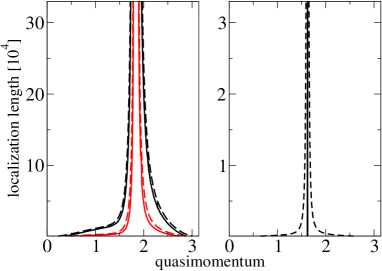
Figure 1: (color online) Anderson localization length obtained from transfer matrix calculations (solid lines) and from (III) (dashed lines). Left panel: Anderson localization length as a function of quasimomentum for two sets of diagonal and off-diagonal disorder amplitude: $\{V_{0}=0.05,\gamma=0.05\}$ (black) and $\{V_{0}=0.1,\gamma=0.1\}$ (red). Filling $\tilde{\rho}=1/3$. Right panel: Anderson localization length as a function of quasimomentum from transfer matrix calculation (black solid line) for diagonal disorder amplitude $V_{0}=0.1$, off-diagonal disorder amplitude $\gamma=0.9$ and occupation $\tilde{\rho}=1/3$. For comparison with (III) we present analytical expression (black dashed line).

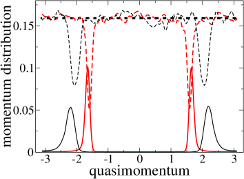
Figure 2: (Color online) Horizontal dotted thick line represents the initial wave packet momentum distribution. Solid lines present momentum distribution of wave function outside area of the disorder while dashed line the distribution of momenta that remain in the system. $N=1000$ lattice sites are considered with filling $\tilde{\rho}=1/3$. Two cases are plotted. The data for diagonal and off-diagonal amplitudes $V_{0}=0.1$, $\gamma=0.5$ are represented by red (thick) curves while those for $V_{0}=0.5,\gamma=0.3$ by black (thin) lines. The evolution time is $t=1000$. The position of dips in momentum space agree with position of transparent mode $k_{t}\approx 1.64$ and $k_{t}\approx 2.08$ respectively. One can observe two peaks in the momentum distributions of escaped atoms. Due to a marginal difference in the dispersion relation between in and outside of the disorder, the positions of peaks and dips are slightly shifted. These results are obtained as the average over $1000$ disorder realizations.

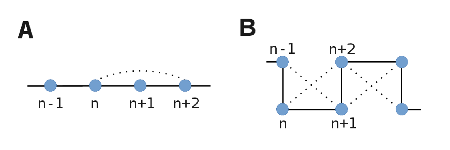
Figure 3: Panel (a): One dimensional gas on a lattice with nearest neighbor hopping (solid line) and next-nearest neighbor hopping (dotted line). Panel (b): The same system can be viewed and described differently, namely as a stripe with non uniform tunneling. The advantage is that the hopping of particles takes place between neighboring slices only.

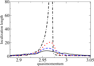
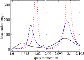
Figure 4: (color online) Anderson localization length as a function of quasimomentum for diagonal disorder $V_{0}=1.95$ (top panel), $V_{0}=1$ (right bottom) and $V_{0}=0.1$ (left bottom), $\gamma=0.9$, occupation $\tilde{\rho}=1/3$. The value of the next nearest neighbor hopping is $t^{\prime}=0.01$ (black solid line), $t^{\prime}=0.005$ (blue dashed line), $t^{\prime}=0.0025$ (red dotted line) and $t^{\prime}=0.0005$ (black dashed-dotted line). The resonance diminishes when $t^{\prime}$ grows. The effect is the strongest for $V_{0}=1.95$ because we are close to a regime without a delocalized mode.

IV Next-nearest neighbor tunnelings

For lattice depths $U\approx 10$-$20\,E_{R}$, where $E_{R}$ is the lattice recoil energy and the typical optical laser wavelengths, next-nearest neighbor hopping amplitude $t^{\prime}$ ranges between $0.01$-$0.001$, as can easily be estimated with appropriate Wannier functions. This is why in typical situations long range hopping is often negligible. Still let us add the next-nearest neighbor tunneling term to the Hamiltonian (1)

$$H\rightarrow H+t^{\prime}\sum_{i}(a^{\dagger}_{i}a_{i+2}+h.c.)\,.$$ (13)

Under the same unitary transformation (3) and after time averaging we obtain the effective Hamiltonian in the form of (5) plus the additional term reading

$$\sum_{i}t^{\prime}_{i}(a^{\dagger}_{i}a_{i+2}+h.c.)\,$$ (14)

with $t^{\prime}_{i}=t^{\prime}\mathcal{J}_{0}\left(\frac{V_{0}}{\omega}(\epsilon_{i+2}-\epsilon_{i})\right)$. We numerically calculate Anderson localization length for this new effective Hamiltonian. The method we use is applicable to finite but arbitrarily long-range hopping. The transfer matrix approach is not directly applicable so we transform the problem from a one dimensional to a two dimensional stripe. This could be achieved with a simple winding of a string, see Fig. 3. In a stripe all particle hoppings are between the neighboring slices, which simplifies numerical calculations.

In the Appendix we present the derivation of the equation for a Green’s function between the first and the last slice of the stripe. Knowing the Green’s function we can easily calculate the localization length Oseledec (1968); MacKinnon and Kramer (1983).

As exemplary parameters for numerical analysis we choose $V_{0}=\{1.95,1,0.1\}$ and $\gamma=0.9$ in order to obtain a regime where a next-nearest-neighbor hopping significantly affects the dynamics of the system. The results are presented in Fig. 4. We observe that even extremely small values of $t^{\prime}$ significantly affect the resonance. The presence of a small but non-zero next-nearest-neighbor tunneling $t^{\prime}$ significantly reduces the localization length for the transparent mode $k_{t}$ due to a non-zero probability that a mobile particle scatters back on a frozen particle through a next-nearest-neighbor hopping. This process can appear when two frozen particles are separated by a single site. Indeed, when we exclude such configurations, the resonance reappears. In deep lattices next-nearest-neighbor tunneling also reduces the localization length for the transparent mode, but the effect is weaker and may not affect the selective emission due to a finite optical lattice size (when this size is smaller than the localization length).

V Conclusions

In this paper we proposed a method to realize a controllable off-diagonal disorder with binary random potential resulting from time-periodic modulation of interactions between mobile and frozen particles in an optical lattice. Since no interactions between mobile particles are taken into account they may be assumed to be spinless (spin-polarized) fermions. One could also imagine a scheme with bosons with interactions tuned off by some microwave or optical Feshbach resonance Chin et al. (2010) (note that we already assume using a magnetic field for a standard Feshbach tuning of different species interactions so this method cannot be used simultaneously to control light-light particle collisions). The presented method allows us to obtain models with strong off-diagonal and weak diagonal disorder in a broad regime of relative (off)-diagonal disorder amplitudes. In a regime of weak off-diagonal disorder, an analytical expression for the Anderson localization length is in very good agreement with numerical simulations. Moreover, we indicate how DRDM with random hopping can work as a tunable band-pass filter for matter-waves. The momentum of escaped atoms reveal narrow peaks in the position of the transparent mode in momentum space while momentum distribution of the Anderson localized atoms reveals dips whose positions agree with former peaks. We indicate the importance of the next-nearest-neighbor hopping for the localization length of the resonant extended mode appearing within dual dimer random model for strong diagonal disorder.

VI Ackowlegments

We are grateful to D. Delande, O. Dutta and K. Sacha for encouraging discussions and for critical reading of the manuscript. We acknowledge a support of the Polish National Science Centre via project DEC-2012/04/A/ST2/00088. AK acknowledges support in a form of a special scholarship of Marian Smoluchowski Scientific Consortium Matter Energy Future from KNOW funding.

VII Appendix A:Hamiltonian approach to Anderson localization length

To find the localization length starting from the map (10) Flores (1989); Tessieri and Izrailev (2001); Izrailev et al. (1995) it is more convenient to express it in the action-angle variables $(r,\theta)$ using the transformation $x=r\sin(\theta)$, $p=r\cos(\theta)$:

$$\left\{\begin{matrix}\sin(\theta_{i+1})=D^{-1}_{i}(\sin(\theta_{i}-k)-A_{i}\sin(\theta_{i})\sin(k))\\ \cos(\theta_{i+1})=D^{-1}_{i}(\cos(\theta_{i}-k)+A_{i}\sin(\theta_{i})\cos(k))\end{matrix}\right.,$$ (15)

where

$$D_{i}\equiv\frac{r_{i+1}}{r_{i}}=\sqrt{1+2A_{i}\sin(2\theta_{i})+A^{2}_{i}\sin^{2}(\theta_{i})}.$$ (16)

We define Anderson localization length as

$$\lambda^{-1}=\lim_{N\to\infty}\frac{1}{N}\sum_{i=1}^{N}\ln D_{i},$$ (17)

and after the expanding logarithm to the second order in $A_{i}$ we get

$$\lambda^{-1}=\frac{1}{8}\langle A^{2}_{i}\rangle+\frac{1}{2}\langle A_{i}\sin(2\theta_{i})\rangle,$$ (18)

where $\langle...\rangle$ stands for averaging over $i$. In order to calculate the ’kick-angle’ correlator $\langle A_{i}\sin(2\theta_{i})\rangle$ we expand the map (15) to second order in $\theta_{i}$:

$$\theta_{i}=\theta_{i-1}-k+A_{i-1}\frac{\sin^{2}(\theta_{i-1})}{\sin(k)}$$ (19)

and express $\langle A_{i}\sin(2\theta_{i})\rangle$ in terms of the preceding $\langle A_{i}\sin(2\theta_{i-1})\rangle$ ’kick-angle’ correlator. Let us introduce the correlation of the kick’s strength $A_{i}$ with angle $\theta_{i}$

$$a_{n}=-\frac{2i}{\langle A_{i}^{2}\rangle}e^{2ik}\langle A_{i}e^{2i\theta_{i-n}}\rangle,\\$$ (20)

where $\langle A_{i}^{2}\rangle$ is variance of the $A_{i}$. Multiple applications of eq. (19) to $a_{n}$ give us the recursive relation

$$a_{n-1}=e^{-2ik}a_{n}+q_{n},$$ (21)

where $q_{n}=\langle A_{i}A_{i-n}\rangle/\langle A_{i}^{2}\rangle$ is the autocorrelation of $A_{i}$. From the definition of $a_{n}$ we can notice that

$$\langle A_{i}\sin(2\theta_{i})\rangle=\Re\left(\frac{\langle A_{i}^{2}\rangle}{2}e^{-2ik}a_{0}\right),$$ (22)

where from (21) we obtain $a_{0}=\sum_{n=1}^{\infty}q_{n}e^{-2ik(n-1)}$.

The inverse Anderson localization length $\lambda^{-1}$ takes the form Tessieri and Izrailev (2001)

$$\lambda^{-1}=\frac{\langle A_{i}^{2}\rangle}{8}\left(1+2\sum_{n=1}^{\infty}q_{n}(k)\cos(2kn)\right).\\$$ (23)

In the specific case of DRDM , the variance of $A_{i}$ and the autocorrelation of $A_{i}$ read, respectively

$$\langle A^{2}_{i}\rangle = \frac{\rho}{(1+\rho)^{2}}\frac{(V_{0}+2\gamma(2-\gamma)\cos(k))^{2}}{\sin^{2}(k)},$$

$$q_{n} = (-1)^{n}\rho^{n}$$ (24)

and the approximate expression for the inverse localization length takes the form (III).

VIII Appendix B:Anderson localization length for Hamiltonian with long-range random hopping

In this section we describe a method of calculating localization length in a one dimensional system with long-range tunneling. The idea is to transform the problem from a one dimensional to a two dimensional stripe. It could be achieved with a simple winding of a string, see Fig. 3.

VIII.1 Mapping to a two–dimensional stripe

To start let us consider a one dimensional gas on a string of length $\tilde{N}$. We allow long-range tunneling up to the $M$-th neighboring site. This geometry is equivalent to a two dimensional stripe of length $N=\tilde{N}/M$ and width $M$. The evolution of particles in such a stripe is characterized by a Hamiltonian

$$H(\tilde{N})=\sum_{n=1}^{N}H_{n}+\sum_{n=1}^{N-1}\Big{(}V_{n}+h.c.\Big{)},$$ (25)

where

$$H_{n} = \sum_{m=1}^{M}\epsilon^{(n)}_{m}|n,m\rangle\langle n,m|$$ (26)

$$- \sum_{m=1}^{M-1}\Big{(}J^{(n,n)}_{m,m+1}|n,m\rangle\langle n,m+1|+h.c.\Big{)}$$

is a standard tight binding Hamiltonian for the $n$-th slice and

$$V_{n}=-\sum_{m=1}^{M}\sum_{m^{\prime}=1}^{M^{\prime}}J^{(n,n+1)}_{m,m^{\prime}}|n,m\rangle\langle n+1,m^{\prime}|$$ (27)

describes particles hopping onto the $n$-th slice. $J^{(n,n^{\prime})}_{m,m^{\prime}}$ denotes tunneling between $|n,m\rangle$ and $|n^{\prime},m^{\prime}\rangle$. Suppose now that we add one extra slice to the system. A new Hamiltonian is straightforward

$$H(N+1)=H(N)+H_{N+1}+V_{N}+V_{N}^{\dagger}.$$ (28)

For later convenience, let us define operators

$$H^{0}(N+1) \equiv H(N)+H_{N+1}$$ (29)

$$V(N) \equiv V_{N}+V_{N}^{\dagger},$$ (30)

and finally the Hamiltonian reads

$$H(N+1)=H^{0}(N+1)+V(N).$$ (31)

VIII.2 A recursive equation for a Green’s function

Our goal is to find the Green’s function $G^{+}_{E}(N+1)$ for the Hamiltonian $H(N+1)$. By definition, a Green’s function can be obtained from a resolvent of a Hamiltonian

$$G^{+}_{E}(N+1)=\lim_{\epsilon\rightarrow 0+}G_{E+i\epsilon}(N+1),$$ (32)

where a resolvent satisfies

$$\left(z-H(N+1)\right)G_{z}(N+1)=1.$$ (33)

Let’s start with an equation for a resolvent of $H(N+1)$:

$$G_{z}(N+1)=G_{z}^{0}(N+1)+G_{z}^{0}(N+1)V(N)G_{z}(N+1),$$ (34)

with $G^{0}_{z}$ being a resolvent of $H^{0}$. The resolvent equation (34) can be derived from a simple operator identity

$$\frac{1}{A}=\frac{1}{B}+\frac{1}{B}(A-B)\frac{1}{A}$$ (35)

with a substitution

$$A=z-H(N+1),\quad B=z-H^{0}(N+1).$$ (36)

Since we are interested in transport properties of the system, we need to know the Green’s function matrix elements between the first and the last slice only. Therefore, we want to obtain $\langle 1|G_{z}(N+1)|N+1\rangle$. To simplify the equations let’s introduce a notation:

$$G_{n,m}\equiv\langle n|G_{z}(m)|m\rangle.$$ (37)

From equation (34) we get

$$G_{1,N+1}=G_{1,N}V_{N}\,G_{N+1,N+1},$$ (38)

where we used an observation that

$$G^{0}_{z}(N+1)=G_{z}(N)+\frac{1}{z-H_{N+1}},$$ (39)

which stems from the fact that $H(N)$ and $H_{N+1}$ act in orthogonal subspaces of the Hilbert space, see (29).

In order to get a recursive equation for $G_{1,N}$, we need to calculate $G_{N+1,N+1}$ matrix. It can be obtained from equation (33) by multiplying it from the right side by a projection $P=|N+1\rangle\langle N+1|$, and by $P$ (or $Q=1-P$) from the left side:

$$P(z-H(N+1))(P+Q)G_{z}(N+1)P = P,$$

$$Q(z-H(N+1))(P+Q)G_{z}(N+1)P = 0.$$ (40)

Solving a set of equations (40) one gets

$$G_{N+1,N+1}=\frac{1}{z-H_{N+1}-V_{N}^{\dagger}G_{N,N}V_{N}}.$$ (41)

Combining equations (38) and (41)

$$G_{1,N+1}\left(z-H_{N}+1-V_{N}^{\dagger}G_{N,N}V_{N}\right)=G_{1,N}V_{N}$$ (42)

and, again from (38), extracting $G_{N,N}$ we finally obtain a recursive equation:

$$A_{N+2}=(E-H_{N+1})V_{N}^{-1}A_{N+1}-V_{N}^{\dagger}V_{N-1}^{-1}A_{N},$$ (43)

with $A_{N}=G^{-1}_{1,N-2}$ . The initial values of $A_{N}$ are not relevant, but it is convenient to choose them as

$$A_{0}=0,\quad A_{1}=V_{0}.$$ (44)

In equation (43) there is no singularity, hence we could replace $z$ with $E$. From this equation we can calculate $G_{1,N}$, which is connected with the localization length of the system.

VIII.3 Calculation of the Anderson localization length

The Anderson localization length $\lambda_{M}$ in a stripe of width $M$ is defined as

$$\frac{2}{\lambda_{M}}=-\lim_{n\rightarrow\infty}\frac{1}{n}\ln\mbox{Tr}|G_{1,n}|^{2}.$$ (45)

Since our system is in fact one dimensional the localization length should not depend on the length of the stripe. When a particle reached the $n$-th slice it covered $\tilde{n}=M\cdot n$ lattice sites. Hence, the localization length $\lambda$ in one dimension equals $\lambda=M\lambda_{M}.$

The localization length can be obtained from the recursive equation (43). We solve the equation iteratively. The problem with this equation is that the elements of $A_{n}$ grow exponentially for large $n$, so it requires some regularization. Therefore, in each step we multiply the both sides of the equation by some matrix $R_{n}$. Starting from $n=1$ and defining $A^{(1)}_{k}\equiv A_{k}R_{1}$

$$A_{3} = (E-H_{2})V_{1}^{-1}A_{2}-V_{1}^{\dagger}V_{0}^{-1}A_{1}\;\Big{|}\times R_{1}$$

$$A_{3}^{(1)} = (E-H_{2})V_{1}^{-1}A_{2}^{(1)}-V_{1}^{\dagger}V_{0}^{-1}A_{1}^{(1)}.$$ (46)

To avoid the exponential growth we put $R_{1}=A_{2}^{-1}$ and

$$A_{3}^{(1)}=A_{3}A_{2}^{-1},\quad A_{2}^{(1)}=1,\quad A_{1}^{(1)}=A_{1}A_{2}^{-1}.$$ (47)

We repeat this procedure in every iteration so that $A_{k}^{(n)}=A_{k}^{(n-1)}R_{n}$, with $R_{n}=\left[A^{(n-1)}_{n+1}\right]^{-1}$, satisfies

$$A_{n+2}^{(n)}=(E-H_{n+1})V_{n}^{-1}-V_{n}^{\dagger}V_{n-1}^{-1}A_{n}^{(n)}.$$ (48)

Let us also define a matrix

$$B^{(n)}=B^{(n-1)}R_{n}/b_{n},\quad b_{n}=\|B^{(n-1)}R_{n}\|,$$ (49)

where $\|\cdot\|=\sqrt{\mbox{Tr}|\cdot|^{2}}$ is a matrix norm. $B^{(n)}$ matrix turns out to be very useful, because

$$b_{n} = \|B^{(n-1)}R_{n}\|=\frac{1}{b_{n-1}}\left\|B^{(n-2)}R_{n-1}R_{n}\right\|=$$ (50)

$$= \frac{1}{b_{n-1}}\left\|B^{(n-2)}\left[A_{n+1}^{(n-2)}\right]^{-1}\right\|=$$

$$= \frac{1}{b_{n-1}b_{n-2}}\left\|B^{(n-3)}\left[A_{n+1}^{(n-3)}\right]^{-1}\right\|=\ldots\,.$$

Continuing this, we notice that

$$\|A_{n+1}^{-1}\| = b_{1}b_{2}\ldots b_{n},$$ (51)

$$\ln\mbox{Tr}|G_{1,n}|^{2} = 2\left(\ln b_{n+1}+\ldots+\ln b_{1}\right).$$ (52)

The Anderson localization length can be expressed as:

$$\lambda=-M\lim_{n\rightarrow\infty}\frac{n}{c_{n+1}},\quad c_{n+1}=c_{n}+\ln b_{n+1}.$$ (53)

Iterations should be continued until $\lambda$ converges within a desired precision.

References

- Anderson (1958) P. Anderson, Phys. Rev. 109, 1492 (1958).
- Lagendijk et al. (2009) A. Lagendijk, B. van Tiggelen, and D. Wiersma, Phys. Today 62, 24 (2009).
- Mott and Twose (1961) N. F. Mott and W. D. Twose, Adv. Phys. 10, 107 (1961).
- Lee and Ramakrishnan (1985) P. A. Lee and T. V. Ramakrishnan, Rev. Mod. Phys. 57, 287 (1985).
- Ishii (1973) K. Ishii, Suppl. Prog. Theor. Phys. 53, 77 (1973).
- Biddle et al. (2011) J. Biddle, D. J. J. Priour, B. Wang, and S. D. Sarma, Phys. Rev. B 83, 075105 (2011).
- Sepehrinia (2010) R. Sepehrinia, Phys. Rev. B 82, 045118 (2010).
- Eilmes et al. (1998) A. Eilmes, R. A. Romera, and M. Schreiber, Eur. Phys. J. B 1, 29 (1998).
- Yamada (2004) T. Yamada, H. Fukui, Nucl. Phys. B 679, 632 (2004).
- Bloch et al. (2008) I. Bloch, J. Dalibard, and W. Zwerger, Rev. Mod. Phys. 80, 885 (2008).
- Jaksch and Zoller (2005) D. Jaksch and P. Zoller, Ann. Phys. 315, 52 (2005).
- Lewenstein et al. (2012) M. Lewenstein, A. Sanpera, and V. Ahufinger, Ultracold Atoms in Optical Lattices: Simulating Many-Body Quantum Systems (Oxford University Press, 2012).
- Eckardt et al. (2005) A. Eckardt, C. Weiss, and M. Holthaus, Phys. Rev. Lett. 95, 260404 (2005).
- Lignier et al. (2007) H. Lignier, C. Sias, D. Ciampini, Y. Singh, A. Zenesini, O. Morsch, and E. Arimondo, Phys. Rev. Lett. 99, 220403 (2007).
- Struck et al. (2011) J. Struck, C. Ölschläger, R. Le Targat, P. Soltan-Panahi, A. Eckardt, M. Lewenstein, P. Windpassinger, and K. Sengstock, Science 333, 996 (2011).
- Chin et al. (2010) C. Chin, R. Grimm, P. Julienne, and E. Tiesinga, Rev. Mod. Phys. 82, 1225 (2010).
- Struck et al. (2012) J. Struck, C. Ölschläger, M. Weinberg, P. Hauke, J. Simonet, A. Eckardt, M. Lewenstein, K. Sengstock, and P. Windpassinger, Phys. Rev. Lett. 108, 225304 (2012).
- Windpassinger and Sengstock (2013) P. Windpassinger and K. Sengstock, Rep. Prog. Phys. 76, 086401 (2013).
- Sacha et al. (2012) K. Sacha, K. Targońska, and J. Zakrzewski, Phys. Rev. A 85, 053613 (2012).
- Eckardt et al. (2010) A. Eckardt, P. Hauke, P. Soltan-Panahi, C. Becker, K. Sengstock, and M. Lewenstein, EPL 89, 10010 (2010).
- Przysiężna et al. (2015) A. Przysiężna, O. Dutta, and J. Zakrzewski, New J. Phys. 17, 013018 (2015).
- Buluta and Nori (2009) I. Buluta and F. Nori, Science 326, 108 (2009).
- Hauke et al. (2012) P. Hauke, M. Cucchietti, F., L. Tagliacozzo, I. Deutsch, and M. Lewenstein, Rep. Prog. Phys. 75, 082401 (2012).
- Billy et al. (2008) J. Billy, V. Josse, Z. Zuo, A. Bernard, B. Hambrecht, P. Lugan, D. Clément, L. Sanchez-Palencia, P. Bouyer, and A. Aspect, Nature 453, 891 (2008).
- Aubry and André (1980) S. Aubry and G. André, Ann. Israel Phys. Soc. 3, 133 (1980).
- Roati et al. (2008) G. Roati, C. D’Errico, L. Fallani, M. Fattori, C. For, M. Zaccanti, G. Modugno, M. Modugno, and M. Inguscio, Nature 453, 895 (2008).
- Aspect and Inguscio (2009) A. Aspect and M. Inguscio, Phys. Today 62, 30 (2009).
- Modugno (2010) G. Modugno, Rep. Prog. Phys. 73, 102401 (2010).
- Jendrzejewski et al. (2012) F. Jendrzejewski, A. Bernard, K. Mueller, C. Patrick, V. Josse, M. Piraud, L. Pezze, L. Sanchez-Palencia, A. Aspect, and P. Bouyer, Nature Phys. 8 (2012).
- Kondov et al. (2011) S. S. Kondov, W. R. McGehee, J. J. Zirbel, and B. DeMarco, Science 334, 66 (2011).
- Gimperlein et al. (2012) H. Gimperlein, S. Wessel, J. Schmiedmayer, and L. Santos, Phys. Rev. Lett. 95, 170401 (2005).
- Massignan and Castin (2006) P. Massignan and Y. Castin, Phys. Rev. A 74, 013616 (2006).
- Gavish and Castin (2005) U. Gavish and Y. Castin, Phys. Rev. Lett. 95, 020401 (2005).
- Ospelkaus et al. (2006) S. Ospelkaus, C. Ospelkaus, O. Wille, M. Succo, P. Ernst, K. Sengstock, and K. Bongs, Phys. Rev. Lett. 96, 180403 (2006).
- Horstmann et al. (2007a) B. Horstmann, J. I. Cirac, and T. Roscilde, Phys. Rev. A 76, 043625 (2007a).
- Krutitsky et al. (2008) K. V. Krutitsky, M. Thorwart, R. Egger, and R. Graham, Phys. Rev. A 77, 053609 (2008).
- (37) T. Roscilde, Phys. Rev. A 77, 063605 (2008).
- Semmler et al. (2010) D. Semmler, K. Byczuk, and W. Hofstetter, Phys. Rev. B 81, 115111 (2010).
- (39) P.D. Antoniou and E. N. Economou, Phys. Rev. B 16, 3768 (1977).
- (40) R. L. Bush, J. Phys. C: Solid State Phys. 8, L547 (1975).
- (41) G. Theodorou and M. H. Cohen, Phys. Rev. B 13, 4597 (1976).
- (42) C.M. Soukoulis and E.N. Economou, Phys. Rev. B 24, 5698 (1981).
- Krey (1983) U. Krey, Z. Phys. B - Condensed Matter 54, 1 (1983).
- Pendry (1982) J. B. Pendry, J. Phys. C: Solid State Phys 15, 5773 (1982).
- (45) F. Delyon, H. Kunz, and B. Souillard, J. Phys. A: Math. Gen. 16, 25 (1983).
- (46) A. Bovier, J. Stat. Phys. 56, 645 (1989).
- Flores (1989) J. Flores, J. Phys.: Condens. Matter 1, 8471 (1989).
- (48) L. Alloatti, J. Phys. Condens. Matter 21, 045503 (2009).
- Piraud et al. (2013) M. Piraud, and L. Sanchez-Palencia, Eur. Phys. J. Special Topics 217, 91 (2013).
- Dunlap et al. (1990) D. H. Dunlap, H.-L. Wu, and P. W. Phillips, Phys. Rev. Lett. 65, 88 (1990).
- (51) F. A. B. F. de Moura and M. L. Lyra, Phys. Rev. Lett. 81, 3735 (1998).
- Zhang et al. (2010) W. Zhang, and S. Ulloa, Phys. Rev. B 69, 153203 (2004).
- (53) R. A. Caetano and P. A. Schulz, Phys. Rev. Lett. 95, 126601 (2005).
- (54) Z. Zhao et al., Phys. Rev. B 75 165117 (2007).
- Schaff et al. (2010) J.-F. Schaff, Z. Akdeniz, and P. Vignolo, Phys. Rev. A 81, 041604 (2010).
- (56) G. Floquet, Gaston Ann. Sci. Ecole Norm. Sup. 12 47 (1883).
- (57) J. H. Shirley, Phys. Rev. 138, B979 (1965).
- (58) S. Rahav, I. Galary, and Sh. Fishman, Phys. Rev. A 68, 013820 (2003).
- (59) A. Eckardt and E. Anisimovac, arXiv:1502.06477.
- (60) M. Bukov, L. D’Alessio, and A. Polkovnikov, arXiv:1407.4803.
- Esmann et al. (2011) M. Esmann, N. Teichmann, and C. Weiss, Phys. Rev. A 83, 063634 (2011).
- Di Liberto et al. (2014) M. Di Liberto, D. Malpetti, G. I. Japaridze, and C. Morais Smith, Phys. Rev. A 90, 023634 (2014).
- Poletti and Kollath (2011) D. Poletti and C. Kollath, Phys. Rev. A 84, 013615 (2011).
- (64) M. Łącki and J. Zakrzewski, Phys. Rev. Lett. 110, 065301 (2013).
- Horstmann et al. (2010) B. Horstmann, S. Dürr, and T. Roscilde, Phys. Rev. Lett. 105, 160402 (2010).
- Rapp et al. (2012) A. Rapp, X. Deng, and L. Santos, Phys. Rev. Lett. 109, 203005 (2012).
- Stasińska et al. (2014) J. Stasińska, M. Łącki, O. Dutta, J. Zakrzewski, and M. Lewenstein, Phys. Rev. A 90, 063634 (2014).
- Muller and Delande (2011) C. A. Muller and D. Delande, Chapter 9 in Les Houches 2009 - Session XCI: Ultracold Gases and Quantum Information (Oxford University Press, 2011).
- Płodzień and Sacha (2011) M. Płodzień and K. Sacha, Phys. Rev. A 84, 023624 (2011).
- Oseledec (1968) V. I. Oseledec, Trans. Mosc. Math. Soc. 19, 197 (1968).
- MacKinnon and Kramer (1983) A. MacKinnon and B. Kramer, Z. Phys. B 53, 1 (1983).
- Tessieri and Izrailev (2001) L. Tessieri and F. Izrailev, Phys. E 9, 405 (2001), ISSN 1386-9477, proceedings of an International Workshop and Seminar on the Dynamics of Complex Systems.
- Izrailev et al. (1995) F. M. Izrailev, T. Kottos, and G. P. Tsironis, Phys. Rev. B 52, 3274 (1995).