On the Dynamics of a Recurrent Hopfield Network

Abstract

In this research paper novel real/complex valued recurrent Hopfield Neural Network (RHNN) is proposed. The method of synthesizing the energy landscape of such a network and the experimental investigation of dynamics of Recurrent Hopfield Network is discussed. Parallel modes of operation (other than fully parallel mode) in layered RHNN is proposed. Also, certain potential applications are proposed.

I Introduction

In the research field of electrical engineering, following the principle of parsimony, many natural as well as artificial systems were modeled as linear systems. However it was realized that many natural/artificial phenomena are inherently non-linear. For instance, many models of neural circuits require non-linear difference/differential equations for modeling their dynamics. Hopfield effectively succeeded in arriving at a model of associative memory based on McCulloch-Pitts neuron. The discrete time Hopfield network represents a non-linear dynamical system.

Hopfield Neural Network spurred lot of research efforts on modeling associative memories (such as the bi-directional associative memory). However, it was realized that the Hopfield neural network is based on undirected graph(for topological representation of network architecture) and hence does not have any directed cycles in the network architecture. Thus, in that sense Hopfield Neural Network (HNN) does not constitute a recurrent neural network. Many recurrent networks, such as Jordan-Elman networks were proposed and studied extensively. After literature survey, we were motivated to propose an Artificial Neural Network (ANN), in the spirit of HNN, but the network architecture is based on a directed graph with directed cycles in it.

Our research efforts are summarized in this paper. In Section-2, a novel real as well as complex Recurrent Hopfield Network is discussed. In Section-3, experimental investigations of Recurrent Hopfield neural Network are discussed. In Section-4, some applications are proposed. The research paper concludes in Section-5.

II Recurrent Hopfield Network(RHN)

Recurrent Hopfield Neural Network (RHNN) is an Artificial Neural Network model. It is a nonlinear dynamical system represented by a weighted, directed graph. The nodes of the graph represent artificial neurons and the edge weights correspond to synaptic weights. At each neuron/node, there is a threshold value. Thus, in summary, a Recurrent Hopfield neural network can be represented by a synaptic weight matrix, M that is not necessarily symmetric and a threshold vector, T. The order of the network corresponds to the number of neurons. Such a neural network potentially has some directed cycles in the associated graph.

Every neuron is in one of the two possible states +1 or -1. Thus, the state space of Nth order Recurrent Hopfield Neural Network (RHNN) is the symmetric N-dimensional unit hypercube. Let the state of ith neuron at time t be denoted by

$$V_{i}(t)\textit{ where }V_{i}(t)\in\{+1\textit{ or}-1\}.$$

Thus, the state of the non-linear dynamical system is represented by the N x 1 vector, $\bar{V}(t)$. The state updation at the ith node is governed by the following equation

$$V_{i}(t+1)=Sign(\sum\limits_{j=1}^{N}M_{ij}V_{j}(t)-T_{i})$$ (1)

where Sign (.) is the Signum function. In other words, $V_{i}(t+1)$ is +1 if the term in the brackets is non-negative, otherwise $V_{i}(t+1)$ is -1. Depending on the set of nodes at which the state updation by Eq.  1  is performed at any time t, the Recurrent Hopfield Neural Network (RHNN) operation is classified into the following modes.

• Serial Mode: The state updation in Eq. 1  is performed exactly at one of the nodes/neurons at time t.

• Fully Parallel Mode: The state updation in Eq. 1  is performed simultaneously at all the N nodes/neurons at time t.

Remark (1).

If the matrix M is symmetric, then the dynamics of Recurrent Hopfield Neural Network (RHNN) is exactly same as the same as that of Ordinary Hopfield Neural Network (OHNN).

For the sake of completeness, we now include the dynamics of Ordinary Hopfield Neural Network (OHNN) with M being a symmetric matrix [1]. In the state space of Ordinary Hopfield Neural Network (OHNN), a non-linear dynamical system, there are certain distinguished states, called the stable states.

Definition II.1.

A state, $\bar{V}(t)$ is called a stable state if and only if

$$\bar{V}(t)=Sign(M\bar{V}(t)-T)$$ (2)

Thus, once the Hopfield Neural Network (HNN) reaches the stable state, irrespective of the mode of operation of the network, the HNN will remain in that state for ever. Thus, there is no further change of the state of HNN once a stable state is reached. The following convergence Theorem summarizes the dynamics of Ordinary Hopfield Neural Network (OHNN). It characterizes the operation of neural network as an associative memory.

Theorem II.1.

Let the pair $N=(M,T)$ specify a Ordinary Hopfield Neural Network (with M being symmetric).Then the following hold true:

[1] Hopfield: If N is operating in a serial mode and the elements of the diagonal of M are non-negative, the network will always converge to a stable state (i.e. there are no cycles in the state space).

[2] Goles: If N is operating in the fully parallel mode, the network will always converge to a stable state or to a cycle of length 2 (i.e the cycles in the state space are of length $\leq 2$).

Remark (2).

It should be noted that in [4], it is shown that the synaptic weight matrix of OHNN can be assumed to be an arbitrary symmetric matrix.

II-A Layered Recurrent Hopfield Neural Network

We now consider a Recurrent Hopfield Neural Network where the neurons (artificial) are organized into finitely many layers (with $\geq 1$ neurons in each layer). Thus the synaptic weight matrix of such a neural network can be captured by a block matrix, W which is not necessarily symmetric. Traditionally, the convergence Theorem associated with Ordinary Hopfield Neural Network (OHNN) (i.e. Theorem  II.1) effectively considered only (i) Serial Mode and (ii) Fully Parallel Mode. But the arrangement of neurons in multiple layers naturally leads to operation of the Hopfield network (Ordinary as well as Recurrent) in other parallel modes of operation. This is accomplished in the following manner:

• It should be noted that the state vector of the Ordinary/Recurrent Hopfield Neural Network at time t can be partitioned into sub-vectors in the following manner.

  $\bar{V}(t)=[\bar{V}^{(1)}(t):\bar{V}^{(2)}(t):...:\bar{V}^{(L)}(t)]\\$ where $\bar{V}^{(1)}(t)$ denotes the state of neurons in layer 1 and L is the number of layers.

  For the sake of notational convenience, suppose that all the ’L’ layers have the same number of neurons in it and state updation at any time instant takes place simultaneously at all nodes in any one layer. This clearly corresponds to parallel mode of operation which is NOT the FULLY PARALLEL MODE (if there is a single neuron in each layer, it corresponds to the serial mode of operation). The state updation in such a ’parallel mode’ can be captured through the following equation: For $1\leq j\leq L$, we have that

  $$\bar{V}^{(j)}(t+1)=Sign(\sum\limits_{k=1}^{L}W_{(j,k)}\bar{V}^{(k)}(t)-\bar{T}_{j})$$

  where $W_{(j,k)}$ is the sub-matrix of W and $\bar{T}_{j}$ is the corresponding threshold vector. It can be shown that there is no loss of generality in assuming that the threshold vector is a zero vector.

  Note: To the best of our knowledge, the dynamics of even OHNN in other parallel modes of operation (not fully parallel) has not been fully investigated.

  Remark (3).

  This idea of layering the neurons enables one to study the dynamics of Recurrent Hopfield Neural Network with various types of directed cycles in it. Theoretical efforts to capture the dynamics of such neural networks are underway. In the Section-3, we summarize our experimental efforts.

• Energy Landscape Synthesis:
  Now we investigate the energy landscape visited by a Recurrent Hopfield Neural Network (RHNN) and relate it to the energy landscape visited by the associated Ordinary Hopfield Neural Network (OHNN).

• Consider the quadratic energy function associated with the dynamics of a RHNN whose synaptic weight matrix is the non-symmetric matrix, W. It is easy to see that

  $$\bar{V}^{T}(n)W\bar{V}(n) =\bar{V}^{T}(n)\left(\frac{W+W^{T}}{2}\right)\bar{V}(n)$$

  $$=\bar{V}^{T}(n)\bar{W}\bar{V}(n)$$

  where $\bar{W}$ is the symmetric matrix associated with W, i.e. symmetric part.

• Now, from the above equation, it is clear that the energy landscape visited by the RHNN with synaptic weight matrix W is exactly same as the energy landscape visited by the OHNN with the symmetric synaptic weight matrix $\bar{W}$. Now, we synthesize the energy landscape of RHNN (or associated OHNN) in the following manner:
  We need the following definition in the succeeding discussion.

Definition II.2.

The local minimum vectors of the energy function associated with W are called anti-stable states. Thus, if u is an anti-stable state of matrix W, then it satisfies the condition

$$u=-Sign(Wu).$$

Using the definitions, we have the following general result.

Lemma II.2.

If a corner of unit hypercube is an eigenvector of W corresponding to positive/negative eigenvalue, then it is also a stable/anti-stable state.

Proof:

Follows from the utilization of definitions of eigenvectors, stable/anti-stable states. Q.E.D.

• Synthesis of Symmetric Synaptic Weight Matrix with desired Energy Landscape:
  Let $\{\frac{\mu_{j}}{N}\}$ where $j\in\{0,1,...,S\}$ be desired positive eigenvalues (with $\mu_{j}$ being the desired stable value) and let $\{X_{j}\}(j\in\{0,1,...,S\})$ be the desired stable states of $\bar{W}$. Then it is easy to see that the following symmetric matrix constitutes the desired synaptic weight matrix of Ordinary Hopfield Neural Network (Using the spectral representation of symmetric matrix $\bar{W}$):

  $$\bar{W}=\sum\limits_{j=1}^{S}\mu_{j}X_{j}X_{j}^{T}$$

  It is clear that the synaptic weight matrix is positive definite. In the same spirit as above, we now synthesize a synaptic weight matrix, with desired stable/anti- stable values and the corresponding stable / anti-stable states. Let $\{X_{j}\}$ where $j\in\{0,1,...,S\}$ be desired orthogonal stable states and $\{Y_{j}\}$ where $j\in\{0,1,...,L\}$ be the desired orthogonal anti-stable states. Let the desired stable states be eigenvectors corresponding to positive eigenvalues and let the desired anti-stable states be eigenvectors corresponding to negative eigenvalues. The spectral representation of desired synaptic weight matrix is given by

  $$W=\sum\limits_{j=1}^{S}\frac{\mu_{j}}{N}X_{j}X_{j}^{T}-\sum\limits_{j=1}^{L}\frac{\beta_{j}}{N}Y_{j}Y_{j}^{T}$$

  where $\mu_{j}$’s are desired positive eigenvalues and $-\beta_{j}$’s are desired negative eigenvalues. Hence the above construction provides a method of arriving at desired energy landscape (with orthogonal stable/anti-stable states and the corresponding positive/negative energy values).

∎

Remark (4).

It can be easily shown that Trace(W) is constant contribution (DC value) to the value of quadratic form $X^{T}WX$ at all corners, X of unit hypercube. Thus, the location of stable/ anti-stable states is invariant under modification of Trace(W) value. Thus, from the standpoint of location/computation of stable/anti-stable states, Trace(W) can be set to zero.

• It should be kept in mind that the dynamics of OHNN with the symmetric synaptic weight matrix $\bar{W}$ is summarized by Theorem II.1, i.e. either there is convergence to stable state or cycle of length 2 is reached. But in the case RHNN with non-symmetric synaptic weight matrix, there may be no convergence or the cycles are of length strictly larger than 2. In the Section-3, we summarize our experimental efforts.

II-B Novel Complex Recurrent Hopfield Neural Network

In research literature on artificial neural networks, there were attempts by many researchers to propose Complex Valued Neural Networks (CVNNs) in which the synaptic weights, inputs are necessarily complex numbers [2, MGZ]. In our research efforts on CVNNs, we proposed and studied one possible Ordinary Complex Hopfield Neural Network (OCHNN) first discussed in [3, RaP], [5-12]. The detailed descriptions of such an artificial neural network requires the following concepts.

1. Complex Hypercube: Consider a vector of dimension ’N’ whose components assume values in the following set $\{1+j1,1-j1,-1+j1,-1-j1\}$.Thus there are points as the corners of a set called the ‘Complex Hypercube”.

2. Complex Signum Function: Consider a complex number ’a + jb’. The ’Complex Signum Function’ is defined as follows:

   $$Csign(a+\textit{j}b)=Sign(a)+\textit{j}Sign(b)$$

In the same spirit of the real valued RHNN, we briefly summarize Complex Recurrent Hopfield Neural Network (CRHNN):

• The complex synaptic weight matrix of such an artificial neural network (CRHNN) need NOT be a Hermitian matrix. The activation function in such a complex valued neural network is the complex signum function. The convergence Theorem associated with Ordinary Complex Hopfield Neural Network (OCHNN) is provided in [3, RaP]. We are experimentally investigating the dynamics of CRHNN.

III Dynamics of Recurrent Hopfield Network:
Experiments

In this section, certain network configurations are simulated with various initial conditions (lying on the unit hypercube) in order to provide insight on the dynamics of the Recurrent Hopfield Networks.

III-A Topology of the networks

The recurrent neural networks whose dynamics are presented in this study have asymmetric synaptic weight matrices with zeros on the diagonal (i.e. no self loops are allowed. As discussed in Remark(4), this assumption can be made without loss of generality). Edge weights (the synaptic weights) are allowed to assume both positive and negative signs. The size of the network (i.e. number of neurons) directly determines the size of synaptic weight matrix. In the experiments, we are going to investigate three cases: synaptic weight matrices with (i) both positive and negative, (ii) only positive and (iii) only negative entries.

III-B Initialization of the network

A Recurrent Hopfield Network, in general, can be randomly initialized in a state s where

$$\textit{s}\in\Psi.$$

$\Psi$ is the state space and

$$\left|\Psi\right|=2^{n}.$$

The size of the state space exponentially increases as the number of neurons are increased. In order to reduce the computational overhead, the number of initial states utilized are limited to a maximum of 1024.

• The decimals numbers in the range [0,1024) are converted to binary and then all 0’s are mapped to -1’s (From this point on, states are going to be referred by using their decimal values).

III-C Modes of operation in experiments

During the experiments, both parallel and serial modes are tested. However, serial mode results in two specific cases. The first is the case where network converges and the second is when there is a cycle of 2 as iterations proceed. On the other hand, parallel mode exhibits more interesting outcomes. Hence, the focus during the experiments have been placed on this update mode.

III-D Results

III-D1 Convergence and cycles

Networks with various polarities of synaptic connections behave expectedly in different manners. The experiments have led to certain types of observations in terms of convergence and cycle characteristics. In vast majority of trials, it has been observed that given an initial state from $\Psi$, the network either converges to a single state or converges into a certain pattern of cycle in multiple iterations.

$$\left(\begin{array}[]{ccccccc}0&11&13&-15&6&-8&-12\\ -20&0&5&-5&4&-16&15\\ 5&-17&0&7&13&13&-6\\ 10&8&-9&0&1&-19&10\\ 4&19&17&-3&0&5&-8\\ -11&-20&9&5&-7&0&16\\ -12&4&2&1&-17&13&0\\ \end{array}\right)$$

Figure 1: Toy synaptic weight matrix

• In networks with both positive and negative synaptic connections, depending on the network size, convergence can take place immediately if the initial state is located in a small proximity to one of the basins of attraction in the energy landscape. However simple generalization of the network dynamics is not possible. The network can be led to certain cycles which are of various lengths. One main observation is that a collection of distinct initial states can be driven into one or more different cycles. This result is interesting since it may imply that a Recurrent Hopfield Network can be used as a function to map signals into certain common cycles. To illustrate the possible state transitions, the network in Figure1 is to be used.

• When parallel mode of update is applied on this network, the results revealed that there exist 6 cycles in which the RHNN loops given all possible initializations. In this mode, length of the cycles varied between 2 and 4 while in the serial mode of operation, the network reached cycles of length of at most two. Furthermore, it often converged to certain minima points in state space. To note, the cycles of length 1 are used to refer to the stable states. The observed cycles, following the naming convention provided previously, are listed in TABLE I.

• If the non-symmetric synaptic weight matrix is non-negative or non-positive, it is observed that the network converges to a single state or to a cycle of length 2.

• If the non-symmetric synaptic weight matrix has positive and negative elements, it is observed that the cycles are of length strictly equal or larger than 2.

• It is observed that in the case of various RHNNs, there are more than one directed cycles in the state space (reached with a change of initial conditions).

• In some special cases a single cycle is reached.

• The simulations show that the networks of mixed-polarity connections are favoring certain states or combinations of the whole possible state space. The parallel mode yielded that inputs that are close in terms of Hamming distance usually go through the same cycles or end up at certain stable states.

• Larger networks with more than 20 neurons are observed to fail to reach at detectable patterns or single state in the parallel mode within reasonable number of iterations.

Next section will focus on the energy values associated with various states. The energy values may be useful to make better conclusions on the observations.

TABLE I: The cycles for the toy example

Mode	Cycles
Parallel	35, 58-69, 42-5, 21-106, 22-119-92-94, 85-122
Serial	11, 35, 36, 41, 45, 57, 61, 63, 64, 66, 70, 86,
	91, 92, 100-12, 27-115, 118-112, 118-31

III-E Energy of the Network during cycles and convergence

The Recurrent Hopfield Networks experimented in this study exhibit two characteristics. First characteristic is that the network reaches a constant energy value when it gets trapped in a single state or a set of states (a cycle). The second characteristic is that the energy of the network fluctuates around a certain DC value. The latter has been observed to occur in cycles only. The typical energy states of the toy example during 128 trials are given in figures Figure2 - Figure6. It is useful to notice that the network’s energy states (during convergence or cyclic period) which are caused by a collection of distinct initial states are the same recapitulating what has been stated previously.

• In Figure2, a common energy profile of network is shown. Usually, in the toy example, the network configures itself into one of the low energy regions.

• Figure3 and Figure5 shows that the network obtains a steady energy even during the cycles while Figure4 and Figure6 indicates that the network’s energy oscillates as well as the state it assumes on each iteration.

• The observations indicate that larger networks exhibit similar behavior in the parallel mode but with the exception that energy fluctuations are more often present during cyclic period.

• In serial mode of operation, the energy of the network remains same if it undergoes a single state convergence whereas it fluctuates if in a cycle of 2.

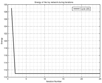
Figure 2: Energy of the network during the cycle 35.

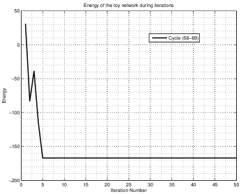
Figure 3: Energy of the network during the cycle 58-69.

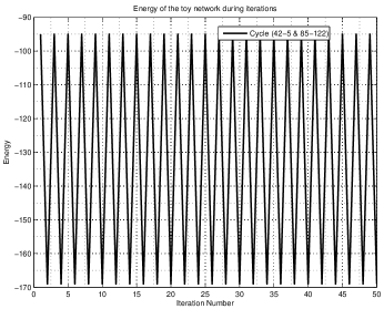
Figure 4: Energy of the network during the cycle 42-5 and 85-122.

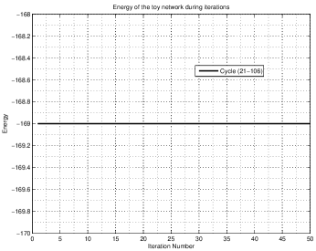
Figure 5: Energy of the network during the cycle 21-106.

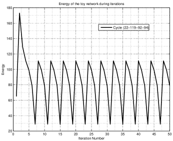
Figure 6: Energy of the network during the cycle 22-119-92-94.

IV Applications

Non-linear dynamical systems exhibit interesting dynamic behavior such as (i) convergence, (ii) oscillations (periodic behavior) and (iii) chaos.

Researchers have identified certain applications (such as cryptography) for interesting non-linear dynamical systems. Specifically neural circuits based on non-linear dynamical systems were identified with certain functional capabilities of biological brains. The authors realized that Recurrent Hopfield Network in this research paper could be capitalized for various applications.

• The main observation is that the cycles of various lengths in the state space could be utilized for applications such as ”MULTI-PATTERN” based associative memory. Based on the length of cycle, a memory utilizing multiple patterns (corners of the hypercube) can be synthesized.

• In the RHNNs investigated, sometimes CONSENSUS to a single cycle is achieved. Thus, such networks could be utilized for memorizing a collection of states corresponding to a cycle.

• In some RHNNs simulated, multiple cycles are reached when the initial condition is varied. Thus, in this case CONSENSUS to multiple memory groups (of states) is achieved.

V Conclusion

In this research paper, our efforts have focused on introducing a novel real/complex valued Recurrent Hopfield Neural Network. In addition, we have shown a method to synthesize a desired energy landscape for such networks. In the experimental section, the dynamics of such real valued Recurrent Hopfield Networks have been investigated in terms of the state transitions and energy. Finally, certain potential applications which exploit the shown properties are proposed.

References

1. J.J. Hopfield, “Neural Networks and Physical Systems with Emergent Collective Computational Abilities,” Proceedings of National Academy Of Sciences, USA Vol. 79, pp. 2554-2558, 1982.
   

2. Mehmet Kerem Muezzinoglu, Cuneyt Guzelis and Jacek M. Zurada, “A new design method for the Complex-valued Multistate Hopfield Associative Memory,” IEEE Transactions on Neural Networks, Vol. 14, No. 4, July 2003.
   

3. G. Rama Murthy and D. Praveen, “Complex-valued Neural Associative Memory on the Complex hypercube,” IEEE Conference on Cybernetics and Intelligent Systems, Singapore, 1-3 December, 2004.
   

4. G. Rama Murthy, “Optimal Signal Design for Magnetic and Optical Recording Channels,” Bellcore Technical Memorandum, TM-NWT-018026, April 1st , 1991.
   

5. G. Rama Murthy and B. Nischal, “Hopfield-Amari Neural Network : Minimization of Quadratic forms,” The 6th International Conference on Soft Computing and Intelligent Systems, Kobe Convention Center (Kobe Portopia Hotel), November 20-24, 2012, Kobe, Japan.
   

6. Akira Hirose, “Complex Valued Neural Networks: Theories and Applications,” World scientific publishing Co, November 2003.
   

7. G. Rama Murthy and D. Praveen, “A Novel Associative Memory on the Complex Hypercube Lattice,” 16th European Symposium on Artificial Neural Networks, April 2008.
   

8. G. Rama Murthy, “Some Novel Real/ Complex Valued Neural Network Models,” Advances in Soft Computing, Springer Series on Computational Intelligence: Theory and Applications, Proceedings of 9th Fuzzy days, September 18-20 2006, Dortmund, Germany.
   

9. G. Jagadeesh, D. Praveen and G. Rama Murthy, “Heteroassociative Memories on the Complex Hypercube,” Proceedings of 20th IJCAI Workshop on Complex Valued Neural Networks, January 6-12 2007.
   

10. V. Sree Hari Rao and G. Rama Murthy, “Global Dynamics of a class of Complex Valued Neural Networks,” Special issue on CVNNS of International Journal of Neural Systems, April 2008.
    

11. G. Rama Murthy, “Infinite Population, Complex Valued State Neural Network on the Complex Hypercube,” Proceedings of International Conference on Cognitive Science, 2004.
    

12. G. Rama Murthy, “Multidimensional Neural Networks-Unified Theory,” New Age International Publishers, New Delhi, 2007.