Simple Distributed $\Delta+1$ Coloring in the SINR Model

Abstract

In wireless ad hoc or sensor networks, distributed node coloring is a fundamental problem closely related to establishing efficient communication through TDMA schedules. For networks with maximum degree $\Delta$, a $\Delta+1$ coloring is the ultimate goal in the distributed setting as this is always possible. In this work we propose $\Delta+1$ coloring algorithms for the synchronous and asynchronous setting. All algorithms have a runtime of  $\mathcal{O}(\Delta\log n)$ time slots. This improves on the previous algorithms for the SINR model either in terms of the number of required colors or the runtime and matches the runtime of local broadcasting in the SINR model (which can be seen as a lower bound).

1 Introduction

One of the most fundamental problems in wireless ad hoc or sensor networks is efficient communication. Indeed, most algorithms concerned with the physical or Signal-to-Interference-and-Noise-Ratio (SINR) model consider algorithms to establish initial communication right after the network begins to operate. However, those initial methods of communication are not very efficient, as there are either frequent collisions and reception failures due to interference, or time is wasted in order to provably avoid such collisions and failures. In the case of local broadcasting[1, 2, 3, 4], a multiplicative $\mathcal{O}(\Delta\log n)$ factor is required to execute message-passing algorithms in the SINR model, where $\Delta$ is the maximum degree in the network, cf. Section 2 for a definition. Thus, wireless networks often use a more refined transmission schedule as part of the Medium Access Control (MAC) layer. One of the most popular solutions to the medium access problem are Time-Division-Multiple-Access (TDMA) schedules, which provide efficient communication by assigning nodes to time slots. The main problem in establishing a TDMA schedule can be reduced to a distributed node coloring. Given a node coloring, we can establish a transmission schedule by simply associating each color with one time slot. The node coloring considered in this work ensure that two nodes capable of communicating directly with each other do not select the same color. Note that a TDMA schedule based on such a coloring is not yet feasible in the SINR model. However, a TDMA schedule that is feasible in the SINR model can be computed based on our coloring, for example as shown in [5, 6].

The problem of distributed node coloring dates back to the early days of distributed computing in the mid-1980s. In contrast to centralized node coloring, a $\Delta+1$ coloring is considered to be the ultimate goal in distributed node coloring as it is already NP-complete to compute the chromatic number (i.e., the minimum number of colors required to color the graph) in the centralized setting[7]. There is a rich line of research in this area, however, most of the work has been done for message-passing models like the $\mathcal{LOCAL}$ model. Such models are designed for wired networks and do not fit the specifics of wireless networks.

In the SINR model, wireless communication is modelled based on the signal transmission and a geometric decay of the signal strength. In contrast to graph-based models such as the protocol model, which model interference between nodes as a purely local property, the SINR model accounts for both local and global interference. Furthermore, it has been shown that the protocol model is quite limited in modeling reality[8]. Often, the SINR model is denoted as the physical model due to its common use in electrical engineering. Thus, the algorithms designed for the SINR model are far more realistic and fit the specifics of wireless networks better.

In this work, we use two simple and very well-known algorithms (covered for example in [9]) designed for message-passing models, and show that we can efficiently execute the algorithms in the SINR model. However, this cannot be achieved by a simple simulation of each round of the message passing algorithm by one execution of local broadcasting as this results in a runtime of $\mathcal{O}(\Delta\log^{2}n)$ time slots. Instead, we modify both the communication rounds in the SINR model and the algorithms to perfectly fit together. The synergy effect of our careful adjustments is that the coloring algorithm runs in $\mathcal{O}(\Delta\log n)$ time slots, which is asymptotically exactly the runtime of one local broadcast[1]. This matches the runtime of current $\mathcal{O}(\Delta)$ coloring algorithms[5], and improves on current $\Delta+1$ coloring algorithms for the SINR model which require $\mathcal{O}(\Delta\log n+\log^{2}n)$ or $\mathcal{O}(\Delta\log^{2}n)$ time slots[10].

Note that our runtime cannot be achieved using algorithms in the $\mathcal{LOCAL}$ model, as state-of-the-art algorithms for distributed node coloring in the $\mathcal{LOCAL}$ model run in $\mathcal{O}(\log\Delta+2^{\mathcal{O}(\sqrt{\log\log n})})$ rounds[11] (in general graphs) or $\mathcal{O}(\log^{*}n)$ rounds[12] (in growth bounded graphs) of local broadcasting. Indeed, a lower bound of $\frac{1}{2}\log^{*}n$ for distributed node coloring in the $\mathcal{LOCAL}$ model due to Linial [13] exists. Thus, in contrast to the algorithm proposed in this work, the number of time slots required to execute distributed node coloring algorithms designed for the $\mathcal{LOCAL}$ model in the SINR model must require $\Omega(\log^{*}n)$ local broadcasting executions.

The communication between nodes in our algorithm is based on the local broadcasting algorithm proposed by Goussevskaia et. al.[1]. Thus, we require the nodes to know an upper bound on the maximum number of nodes in a node’s surroundings (which we call proximity area, cf. Section 2), an upper bound on the number of nodes in the network, as well as some model-related hardware constants in order to enable initial communication. Such requirements are common in the SINR model, however, we discuss the case that the number of nodes in the proximity area is not known in Section A.3. We discuss related work and our contributions in the next section.

1.1 Related Work and Contributions

Due to the rich amount of work on distributed node coloring in the message-passing model, we shall only highlight the most efficient algorithms for $\Delta+1$ colorings here. For a more thorough overview we refer to a recent monograph by Barenboim and Elkin [9]. The fastest deterministic algorithm for general graphs is due to Awerbuch et. al. [14] and Panconesi and Srinivasan [15] and runs in $2^{\mathcal{O}(\sqrt{\log n})}$. For moderate values of $\Delta$, another deterministic algorithm with runtime $\mathcal{O}(\Delta)+\frac{1}{2}\log^{*}n$ is due to Barenboim, Elkin and Kuhn [16]. For growth bounded graphs, which generalize unit disk graphs, a deterministic distributed algorithm due to Schneider and Wattenhofer [12] computes a valid $\Delta+1$ coloring in $\mathcal{O}(\log^{*}n)$ rounds. Regarding randomized algorithms, the algorithm on which this work is based was the most efficient $\Delta+1$ coloring algorithm until recently [9, Chapter 10]. The algorithm can be seen as a simple variant of Luby’s maximal independent set algorithm [17]. In recent years the problem received considerable attention which culminated in the currently best randomized algorithm running in $\mathcal{O}(\log\Delta+2^{\mathcal{O}(\sqrt{\log\log n})})$ due to Barenboim et. al. [11].

In wireless networks, the SINR model received increasing attention first in the electrical engineering community, and was picked up by the algorithms community due to a seminal work by Gupta and Kumar [18]. An overview of works regarding transmission scheduling in the SINR model can be found in a survey by Goussevskaia, Pignolet and Wattenhofer [19]. Other results cover Broadcasting [20, 21], Local Broadcasting[1, 2, 3, 4] and backbone construction[22]. Regarding distributed node coloring in the SINR model Derbel and Talbi [5] show that a distributed node coloring algorithm due to Moscibroda and Wattenhofer [23, 24] can be adapted to the SINR model. They provide an algorithm that computes an $\mathcal{O}(\Delta)$ coloring in $\mathcal{O}(\Delta\log n)$ time slots. The algorithm first computes a set of leaders using a maximal independent set (MIS, cf. Section 2) algorithm, then leader nodes assign colors to non-leaders, which again compete for their final color with a restricted number of neighboring nodes that may have received the same assignment. Yu et. al. [10] propose two $\Delta+1$ coloring algorithms that do not require the knowledge of the maximum node degree $\Delta$. Their first algorithm runs in $\mathcal{O}(\Delta\log n+\log^{2}n)$ time slots and assumes that nodes are able to increase their transmission power for the computation. This prevents conflicts between non-leader nodes by allowing the set of leaders to directly communicate to other leaders outside the transmission region and thus coordinating the assignment process. Their second algorithm does not require this assumption and runs in $\mathcal{O}(\Delta\log^{2}n)$ time slots.

Our main contributions are

• a very simple algorithm to compute a $\Delta+1$ algorithm in  $\mathcal{O}(\Delta\log n)$ time slots in the synchronous setting;

• an abstract method that has the potential of improving the runtime of other randomized algorithms in the SINR model by a  $\log n$ factor; and

• an asynchronous color reduction scheme, which, combined with known coloring algorithms computes a $\Delta+1$ coloring in  $\mathcal{O}(\Delta\log n)$ time slots.

The coloring algorithms improve current algorithms in the same setting (cf. Derbel and Talbi [5]) regarding the number of colors the declared goal of $\Delta+1$, while the runtime is matched. Other $\Delta+1$ coloring algorithms in the SINR model require at least $\mathcal{O}(\Delta\log n+\log^{2}n)$ time slots (under not comparable assumptions). The method to improve the runtime by a $\log n$ factor carefully combines the uncertainty in randomized algorithms with the uncertainty in the SINR model to handle them combined in the analysis. For more details, we refer to the Analysis of Algorithm 1 in Section 4.1.

Roadmap: In the next section we state the model along with required definitions. Communication results in the SINR model required in the algorithm are stated in Section 3. In Section 4 the algorithms for the synchronous setting are described and analyzed. The color reduction scheme is generalized to the asynchronous setting in Section 5.

2 Model and Preliminaries

Let us formulate some notation before defining the coloring problem. The Signal-to-Interference-and-Noise-Ratio (SINR) model is used to model whether transmission in a wireless network can be successfully decoded at the intended receivers or not. We say that a transmission from a sender to a receiver is feasible if it can be decoded by the receiver. In the SINR model it depends on the ratio between the desired signal and the sum of interference from other nodes plus the background noise whether a certain transmission is successful. Let each node $v$ in the network use the same transmission power $P$. Then a transmission from $u$ to $v$ is feasible if and only if

$$\frac{\frac{P}{\operatorname{dist}(u,v)^{\alpha}}}{\sum_{w\in I}\frac{P}{\operatorname{dist}(w,v)^{\alpha}}+\operatorname{N}}\geq\beta,$$

where $\alpha,\beta$ are constants depending on the hardware, $\operatorname{N}$ reflects the environmental noise, $\operatorname{dist}(u,v)$ the Euclidean distance between two nodes $u$ and $v$, and $I\subseteq V$ is the set of nodes transmitting simultaneously to $u$. The broadcasting range $r_{B}$ of a node $v$ defines the range around $v$ up to which $v$’s messages should be received. We denote the set of neighbors of $v$ by $N_{v}:=\{w\in V\backslash\{v\}|\operatorname{dist}(v,w)\leq r_{B}\}$ and $N_{v}^{+}:=N_{v}\cup\{v\}$. Based on the SINR constraint, the transmission range of $r_{T}\leq(\frac{P}{\beta\operatorname{N}})^{1/\alpha}$ is an upper bound for the broadcasting range (with $r_{B}\leq(1-\epsilon)r_{T}$ for a constant $\epsilon>0$, otherwise no spacial reuse is possible). Let the broadcasting region $B_{v}$ be the disk with range $r_{B}$ centered at $v$.

The communication graph $G=(V,E)$ is defined as follows. The set of vertices $V$ in the graph corresponds to the set of nodes in the network, while there is an edge $(u,v)\in E$ if and only if $u$ and $v$ are neighbors (i.e., they are within each other’s broadcasting range). The maximum degree in the network is $\Delta:=\max_{v\in V}|N_{v}|$. Note that since $r_{B}<r_{T}$, a node $v$ may successfully receive transmissions from nodes that are not its neighbors in the communication graph, although successful transmission from those node cannot be guaranteed. As the signal strength decreases geometrically in the SINR model, we can assume that messages from outside the broadcasting range are discarded by considering the signal strength of a received message (wireless communication hardware usually provides this indication as the Received-Signal-Strength-Indication (RSSI) value[25]). In a more practical setting, one could also define the communication graph based on the possible communication between two nodes. For this work we restrict communication of the nodes to the broadcasting range by assuming nodes outside the broadcasting range discard the message. To prove successful communication within the broadcasting range, we need the concept of a proximity range $r_{A}>2r_{B}$ around a node $v$ as introduced in [1]. Let $\Delta^{v}_{A}$ be the number of nodes with distance less than $r_{A}$ to $v$, and $\Delta^{A}:=\max_{v\in V}\Delta^{v}_{A}$. It holds that $\Delta^{A}\in\mathcal{O}(\Delta)$. As further technical details of the proximity range are not required in our analysis, we refer to [1] for the exact definitions.

In the synchronous setting, we assume the nodes to start the algorithm at the same time. We discuss this assumption briefly in Section A.3. In the more realistic asynchronous setting arbitrary wake-up of nodes is allowed and we do not require synchronized time slots; decent clocks, however, are assumed. In our analysis, we shall argue using time slots although the nodes to not have common time slots. As, for example, in [1] communication can be established in asynchronous networks similar to synchronous networks using the aloha trick.

We call two nodes $v,u\in V$ independent if they are not neighbors. A set $S\subseteq V$ such that the nodes in $S$ are pairwise independent is called independent set. Obviously, $S\subseteq V$ is a maximal independent set (MIS) if $S$ is independent and there is no $v\in V\backslash S$ with $S\cup\{v\}$ independent. Denote the set of integers $\{0,\dots,i\}$ by $[i]$. Let us now define the coloring problem. Given a set of nodes $V$ so that each node $v\in V$ has a color  $c_{v}$, and let $d$ be an integer. Then $V$ has a valid $d+1$ coloring, if for each node $v$ holds $\forall v\in N_{v}:c_{v}\not=c_{w}$ and $c_{v}\in[d]$. Observe that in a valid coloring each color in the network forms a independent set.

In the following we introduce the notation required for the analysis of Algorithm 1, which consists of several phases and is described in the next section. We say that two nodes $v,w$ have a conflict if $c_{v}=c_{w}$ and denote the temporary color of $v$ in phase $t$ by $c^{t}_{v}$. The set of nodes that are in a conflict with $v$ in phase $t$ is $X^{t}(v):=\{w\in N_{v}|c^{t}_{v}=c^{t}_{w}\}$. We call $X^{t}(v)$ the conflict set of $v$ in phase $t$. Let us now define some events. The event that $v$ is in a conflict in phase $t$ is $\mathcal{E}^{t}_{\text{confl}}(v):=\exists w\in X^{t}(v)$. Note that it does not matter whether $v$ knows of the conflict or not. The event that a transmission from $v$ to all neighbors $N_{v}$ of $v$ in phase $t$ is successful is $\mathcal{E}^{t}_{\text{succ}}(v)$. A transmission from $v$ to its neighbors in phase $t$ is not successful or fails if at least one neighbor was unable to receive the message. The corresponding event is $\mathcal{E}^{t}_{\text{fail}}(v)$. We replace $\mathcal{E}$ by $\mathbb{P}$ to denote the probability of an event, e.g. $\mathbb{P}^{t}_{\text{succ}}(v)$ instead of $\mathcal{E}^{t}_{\text{succ}}(v)$. Note that although the events $\mathcal{E}^{t}_{\text{succ}}(v)$, and $\mathcal{E}^{t}_{\text{fail}}(v)$ may not be independent of events happening at other nodes, our bounds on the corresponding probabilities $\mathbb{P}^{t}_{\text{succ}}(v)$ and $\mathbb{P}^{t}_{\text{fail}}(v)$ are independent from the node $v$ and possible events at other nodes. Also, our bounds $\mathbb{P}^{t}_{\text{succ}}(v)$ and $\mathbb{P}^{t}_{\text{fail}}(v)$ on these events include the event that $v$ reaches some but not all of its neighbors, as $\mathbb{P}^{t}_{\text{fail}}(v)\leq 1-\mathbb{P}^{t}_{\text{succ}}(v)\leq 1/12$ and $11/12\leq\mathbb{P}^{t}_{\text{succ}}(v)\leq 1$ (see Section 3 for a proof of the bounds).

The nodes use two different transmission probabilities in order to adapt to the requirements of the corresponding algorithms. Probability $p_{1}:=\frac{1}{2\Delta^{A}}$ is used in Algorithm 1, while Algorithm 1 uses $p_{2}:=\frac{1}{180}$. Algorithm 2 uses both transmission probabilities. Let $c$ be an arbitrary constant with $c>1$. Throughout the paper, we use the following constants: $\kappa_{\ell}:=c\lambda\ln n/p_{\ell}$ for $\ell=1,2$, $\kappa_{0}:=\lambda\ln 12/p_{1}$, and $\lambda:=\left(P^{A_{v}}_{\text{none}}\cdot P^{v}_{\text{SINR}}\right)^{-1}$, where $P^{A_{v}}_{\text{none}}=(1/4)^{\mathcal{O}(1)}$ and $P^{v}_{\text{SINR}}=1/2$ to simplify arguments in the SINR model (for more details and a derivation of the probabilities, we refer to Appendix A.2). Note that $\kappa_{0}\in\mathcal{O}(\Delta)$, $\kappa_{1}\in\mathcal{O}(\Delta\log n)$, and $\kappa_{2}\in\mathcal{O}(\log n)$. We shall use the following mathematical fact in our analysis. It can be found, for example, in the mathematical background section of [26].

Fact 1.

For all $t,n\in\mathbb{R}$, such that $n\geq 1$ and $|t|\leq n$ it holds that $\left(1+\frac{t}{n}\right)^{n}\leq e^{t}$.

3 Adaptable Transmission Probabilities in the SINR Model

We shall show in this section that local broadcasting with constant success probability in time reversely proportional to the transmission probability can be achieved. This is extends known results regarding local broadcasting, which guarantee local broadcasting with high probability for a fixed number of time slots. As in these results we require the nodes transmission probability to conform with the requirement that the sum of transmission probabilities from each broadcasting region is at most 1, which is stated in Lemma 2. This local property is used in the following theorem to ensure that both the interference by few local transmissions as well as the summed interference by all globally simultaneous transmissions can be handled.

Lemma 2.

Let all nodes in the network execute Algorithm 1 (or Algorithm 2), and let $v$ be an arbitrary node. Then the sum of transmission probabilities from within $v$’s broadcasting range is at most 1.

The proof is a simple summation over the number of nodes in the broadcasting region and the transmission probabilities used for nodes in the algorithms. Due to space restrictions it is deferred to Appendix A.1. Let us now state the main theorem of this section.

Theorem 3.

Given a network of nodes. Let $v$ be an arbitrary node transmitting with probability $p>0$ in each time slot, and let the sum of transmission probabilities from within each broadcasting region be at most 1. A transmission from $v$ is successful within  $\frac{\lambda\ln 12}{p}$ time slots with probability at least $\frac{11}{12}$.

The proof of the theorem is along the lines of the proof that local broadcasting can be achieved in $\mathcal{O}(\Delta\log n)$ time slots [1]. Thus, we shall only give a sketch of the proof here. For the sake of completeness, an adaptation of the full proof to our theorem can be found in Appendix A.2.

Proof.

The proof is based on two major observations, which are both implied by the fact that the sum of transmission probabilities from within each broadcasting range is bounded by 1.

1. The probability $P^{A_{v}}_{\text{none}}$ that $v$ is the only node in the proximity region that transmits a signal in the current time slot is constant.

2. The probability $P^{v}_{\text{SINR}}$ that the SINR constraint holds for a given transmission of $v$ is constant.

By combining these probabilities with the transmission probability it follows that the probability that $v$ successfully transmits a message to all neighbors in a given time slot is at least $p\cdot P^{A_{v}}_{\text{none}}\cdot P^{v}_{\text{SINR}}$. As we set $\lambda:=\left(P^{A_{v}}_{\text{none}}\cdot P^{v}_{\text{SINR}}\right)^{-1}$, the probability for a successful transmission to all neighbors after $\kappa_{0}=\frac{\lambda\ln 12}{p}$ time slots is at least

$$1-\left(1-\frac{p}{\lambda}\right)^{\frac{\lambda\ln 12}{p}}\geq 1-e^{-\ln 12}\geq 1-\frac{1}{12}\geq\frac{11}{12},$$

which proves the theorem. ∎

A combination of Lemma 2 and Theorem 3 implies the following two results. The first states that in each phase of Algorithm 1, the currently selected color is transmitted to all neighbors with constant probability, which enables us to analyze Algorithm 1 and correctly account for the uncertainty in the message transmission in this algorithm in Section 4.1.

Corollary 4.

Let $v$ be a node in the network executing Algorithm 1. Then $v$ successfully transmits its color to its neighbors with probability $\mathbb{P}^{t}_{\text{succ}}(v)\geq\frac{11}{12}$ in each phase of length $\kappa_{0}\in\mathcal{O}(\Delta)$.

The second result applies to the message transmission in the color reduction scheme of Algorithms 1 and 2. In order to make the lemma applicable to both algorithms, we state the result in a general way. It includes the standard local broadcasting bounds known from [1], but also enables the algorithms to use a more coordinated (and faster) medium access based on the coloring. Local broadcasting achieves successful message transmission from each node in the network in $\mathcal{O}(\Delta\log n)$ time slots, while the more coordinated approach used in the color reduction scheme achieves successful message transmission from a constant number of nodes in each broadcasting region to their neighbors in $\mathcal{O}(\log n)$ time slots.

Lemma 5.

Given a network of nodes. Let $v$ be a node transmitting with probability $p_{\ell}$ in each time slot according to Algorithm 1 or 2. Then a transmission from $v$ is successful within $\kappa_{\ell}$ time slots w.h.p. for $l\in\{1,2\}$.

Proof.

Note that most nodes transmit with probability $p_{1}$ in both algorithms and only few, i.e., a constant number of nodes in each broadcasting range, are allowed to transmit with probability $p_{2}$ simultaneously. Having all nodes transmitting with $p_{1}$ for  $\kappa_{1}\in\mathcal{O}(\Delta\log n)$ time slots is essentially the well-known result on local broadcasting by Goussevskaia et. al. [1]. The transmission probability $p_{2}$ is constant and selected such that the constant number of nodes required by the respective algorithms may use $p_{2}$ without violating Lemma 2.

Similar to the argumentation in Theorem 3, attempting to transmit with probability $p_{\ell}$ for $\kappa_{\ell}$ time slots ($\ell=1,2$) yields a failure probability of at most

$$1-\left(1-\frac{p_{\ell}}{\lambda}\right)^{\kappa_{\ell}}\geq 1-e^{c\ln n}\geq 1-\frac{1}{n^{c}},$$

which completes the proof. ∎

This implies that the communication used in our algorithms is successful with the corresponding probabilities. We shall prove the correctness of our algorithms in the following.

4 Synchronous Setting

The algorithm we propose is at its heart a very simple and well-known randomized coloring algorithm. The underlying approach dates back to an algorithm to compute maximal independent sets by Luby [27], and is covered for example in [9, Chapter 10]. Essentially, this kind of algorithms draw a random color whenever two neighboring nodes have the same color (i.e., there is a conflict between them). However, in contrast to previous algorithms of this kind, we do not assume that successful communication is guaranteed by lower layers. Instead we allow the uncertainty in the randomized algorithm to unite with the uncertainty in the communication in the SINR model, which is jointly handled in the analysis. Thereby we can reduce the number of time slots required for each phase by a $\log n$ factor (from $\mathcal{O}(\Delta\log n)$ for the trivial analysis to $\mathcal{O}(\Delta)$), making this simple approach viable in the SINR model.

Algorithm 1.1: Rand4DeltaColoring for $v$

 

0[-0.80] $F_{v}\leftarrow[4\Delta]$, $c_{v}^{-1}\leftarrow F_{v}.$random()

1 for $t\leftarrow 0;t\leq 6(c+3)\ln n;t\leftarrow t+1$ do // each one phase

      2 if $c^{t-1}_{v}\not\in F_{v}$ then $c^{t}_{v}\leftarrow F_{v}$.rand()

      3  // if conflict, new color else $c^{t}_{v}\leftarrow c^{t-1}_{v}$

      4  // otherwise, keep it $F_{v}\leftarrow[4\Delta]$

      5 Transmit $c^{t}_{v}$ with probability $p_{a}$ for $\kappa_{0}$ time slots

      6 foreach received color $c^{t}_{w}$ from neighbor $w\in N_{v}$ do  $F_{v}\leftarrow F_{v}\backslash\{c^{t}_{w}\}$

      

 

[-0.80] Algorithm 1.2: ColorReduction for node $v$

 

7[-0.80] $F_{v}\leftarrow[\Delta]$

8 foreach color $c_{i}=i\in[4\Delta]$ do

      9 if $c^{t}_{v}\not=i$ then // wait

            10 listen for $\kappa_{2}$ time slots

            11 foreach received color $c_{w}$ from neighbor $w\in N_{v}$ do  $F_{v}\leftarrow F_{v}\backslash{c_{w}}$

            

      13else  // otherwise, select and transmit final color

            14 $c_{v}\leftarrow F_{v}$.random()

            15 Transmit $c_{v}$ with probability $p_{2}$ for $\kappa_{2}$ time slots

            

      

Algorithm 1 RandColoring for node $v$

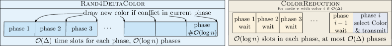
Figure 1: Illustrations of the synchronous Algorithms. Left: Algorithm 1. Right: Algorithm 1.

Our first algorithm (Rand4DeltaColoring, Algorithm 1 and Fig. 1) is a simple, phase-based coloring algorithm. In each phase the node checks whether it knows of a conflict with one of its neighbors. If so, it randomly draws a new color from the set $F_{v}$ of colors not taken in the previous phase. Finally, the phase is concluded by transmitting the current color. This part computes a valid coloring with $4\Delta$ colors in $\mathcal{O}(\log n)$ phases, while each phase takes $\mathcal{O}(\Delta)$ time slots. Our main contribution regarding this algorithm lies in the analysis, as phases of length $\mathcal{O}(\Delta)$ are not sufficient to guarantee successful message transmission. This allows us to save a $\log n$ factor, at the cost of handling uncertain message transmission in the analysis of the algorithm.

Assume the nodes have agreed on a valid coloring with $d$ colors. The second algorithm (ColorReduction, Algorithm 1 and Fig. 1) improves the coloring by reducing the number of colors to $\Delta+1$. The general scheme is that the nodes in the networks gradually replace their color by a color from $[\Delta]$. In each phase, the nodes of exactly one color select a new color from $[\Delta]$ and broadcast their selection to their neighbors. As each color forms an independent set, those nodes are free to select a color that is not yet taken in their neighborhood and communicate the selected color to the neighbors without introducing a conflict. In order to make the algorithm efficient in the SINR model, we utilize the given coloring to improve the communication efficiency by building a tentative schedule for the transmissions of each node. As nodes of exactly one color attempt to transmit in each phase, the nodes of this color can successfully transmit their (new) color selection to neighboring nodes with high probability in only $\mathcal{O}(\log n)$ time slots instead of $\mathcal{O}(\Delta\log n)$. As each node that selects a final color from $[\Delta]$ knows of its neighbors colors, it can select and communicate its color without introducing a conflict. Overall this algorithm requires $d$ phases to reduce a $d$ coloring to a $\Delta+1$ coloring. As each phase requires $\mathcal{O}(\log n)$ time slots this results in $\mathcal{O}(d\log n)$ time slots.

Our algorithms are combined to compute a $\Delta+1$ coloring from scratch. Directly after finishing the execution of Algorithm 1, the nodes begin executing Algorithm 1 in order to compute a $\Delta+1$ coloring from scratch in $\mathcal{O}(\Delta\log n)$ time slots. Both parts of the algorithm are well-known in the $\mathcal{LOCAL}$ model, however, simply executing the algorithms in the SINR model leads to a runtime $\mathcal{O}(\Delta\log^{2}n+\Delta^{2}\log n)$ time slots. Due to the careful combination of the algorithms with specifics of the SINR model, along with handling the uncertainty of successful message transmission both in the algorithm and the analysis, we are able to execute both parts of the algorithm in $\mathcal{O}(\Delta\log n)$ time slots. Thus, Algorithm 1 solves the $\Delta+1$ coloring problem in $\mathcal{O}(\Delta\log n)$ time slots, which matches the runtime of one execution of local broadcasting in the SINR model.

4.1 Analysis of Rand4DeltaColoring

Despite the fact that the underlying coloring algorithm is well-known, our analysis is new and quite involved. The main reason for this is the uncertainty in whether a message is successfully delivered in one phase of Algorithm 1. In contrast to guaranteed message delivery based for example on local broadcasting, message delivery with constant probability can be achieved a logarithmic factor faster, see Section 3. However, this reduction in runtime comes at a cost: While in the guaranteed message delivery setting, a node can finalize its color once a phase without a conflict happened, this is not possible in our setting, as we cannot guarantee the validity of the colors even if a node did not receive a message implying a conflict in one phase due to message transmission with only constant probability. Nevertheless, we can show that after $\mathcal{O}(\log n)$ phases of transmitting the selected color and resolving eventual conflicts, the coloring is valid in the entire network w.h.p.

Our formal analysis shall be structured as follows. We show in this section that the probability for a conflict indeed reduces by a constant factor in each phase. This is the foundation for the result that the first part of our coloring algorithm computes a valid $4\Delta$ coloring in $\mathcal{O}(\Delta\log n)$ time slots w.h.p., which is the main result in this section. In Section 4.2 we show that Algorithm 1 transforms a valid $4\Delta$ coloring into a valid $\Delta+1$ coloring with high probability and conclude that the total runtime of Algorithm 1 is $\mathcal{O}(\Delta\log n)$ time slots.

In order to prove correctness of Algorithm 1 (Rand4DeltaColoring) we shall first bound the probability of a conflict propagating from one phase of the algorithm to the next. This enables us to show that each node that participates in the algorithm selects a valid color. Based on the probability that a node $v$ has a conflict in phase $t$, there are only two cases that may lead to a conflict at $v$ in phase $t+1$:

1. $v$ had a conflict in phase $t$, and it did not get resolved (either due to being unaware of the conflict or since the new color implies a conflict as well).

2. a neighbor of $v$ had a conflict in phase $t$ and introduced the conflict by randomly selecting $v$’s color.

We shall show that the probability for both cases is constant (see Lemma 7). Thus, after $\mathcal{O}(\log n)$ phases it holds with high probability that a valid color has been found. Let us now state the main result of this section.

Theorem 6.

Let all nodes start executing Algorithm 1 simultaneously. After the execution, all nodes have a valid color with probability $1-1/n^{c}$.

Before proving this result let us formulate and prove the following lemma, which lays the foundations to prove Theorem 6. In this lemma we bound the probability of a conflict in phase $t+1$ based on the probability of a conflict in phase $t$.

Lemma 7.

Let $v$ be an arbitrary node and $\mathbb{P}^{t}_{\text{confl}}(v)$ the probability of a conflict at $v$ in phase $t$. Then the probability of a conflict at $v$ in phase $t+1$ is at most

$$\mathbb{P}_{\text{confl}}^{t+1}(v)\leq\frac{5}{6}\cdot\max_{w\in N_{v}}\mathbb{P}^{t}_{\text{confl}}(w).$$

Proof.

We shall prove the lemma by considering the two cases that may lead to a conflict at node $v$ in phase $t+1$. The first case is that $v$ has a conflict with at least one of its neighbors. Depending on which transmissions are successful there are 3 subcases. Note that $\rightarrow$ denotes $\mathcal{E}^{t}_{\text{succ}}(v)$, while $\leftarrow$ denotes $\exists w\in X^{t}(v):\mathcal{E}^{t}_{\text{succ}}(w)$—with negations accordingly.

1. It is not guaranteed that any of the conflict partners know of the conflict, as the transmissions from $v$ and the nodes in the conflict set $X^{t}(v)\neq\emptyset$ failed at least partially. There is at least one neighbor $u\in X^{t}(v)$ that failed to transmit its color successfully to $v$, which happens with probability $\mathbb{P}^{t}_{\text{fail}}(u)$. Combined with $v$’s failure to transmit its color successfully, case 1(a) happens with probability at most $\mathbb{P}^{t}_{\text{confl}}(v)(\mathbb{P}^{t}_{\text{fail}}(v)\Pr(\not\leftarrow))$ $\leq\mathbb{P}^{t}_{\text{confl}}(v)\mathbb{P}^{t}_{\text{fail}}(v)\mathbb{P}^{t}_{\text{fail}}(u)\leq\mathbb{P}^{t}_{\text{confl}}(v)(1/12)^{2}$. If any conflict partner knows of the conflict, the conflict would be resolved with a certain probability (as in the following cases). However, as this is not guaranteed, we account for the worst case, which is that the conflict is not resolved and propagates to the next phase. Note that since this case happens only with a small probability, we have shown that the total probability of case (a) and conflict at $v$ in phase $t+1$ is small.

2. All nodes in $X^{t}(v)$ failed to transmit successfully, but $v$ transmitted successfully to all neighbors. Thus, all nodes in $X^{t}(v)$ know of the conflict, while $v$ might be unaware of it. This case happens with probability at most $\mathbb{P}^{t}_{\text{confl}}(v)\cdot(\mathbb{P}^{t}_{\text{succ}}(v)\cdot\Pr(\not\leftarrow))$. The probability that a node $w\in X^{t}(v)$ selects $v$’s color in phase $t+1$ is at most $\sum_{w\in X^{t}(v)}1/|F_{w}|$ (even if $v$ knows of a conflict and itself selects a new color). This results in an overall probability of at most

   $$\mathbb{P}^{t}_{\text{confl}}(v)\cdot(\mathbb{P}^{t}_{\text{succ}}(v)\cdot\Pr(\not\leftarrow))\cdot\sum_{w\in X^{t}(v)}\frac{1}{|F_{w}|}$$

   $$\leq\mathbb{P}^{t}_{\text{confl}}(v)\left(\prod_{w\in X^{t}(v)}\mathbb{P}^{t}_{\text{fail}}(w)\right)\cdot\sum_{w\in X^{t}(v)}\frac{1}{|F_{w}|}$$

   $$\overset{x:=|X^{t}(v)|}{\leq}\mathbb{P}^{t}_{\text{confl}}(v)\left(\mathbb{P}^{t}_{\text{fail}}\right)^{x}\cdot\frac{x}{3\Delta}$$

   $$\leq\frac{1}{3\Delta}\mathbb{P}^{t}_{\text{confl}}\cdot x\left(\frac{1}{12}\right)^{x}\leq\frac{1}{24}\mathbb{P}^{t}_{\text{confl}}$$

   where the first inequality holds since the event $\not\leftarrow$ is equivalent to $\forall w\in X^{t}(v):\mathcal{E}^{t}_{\text{fail}}(w)$ and $\mathbb{P}^{t}_{\text{succ}}(v)\leq 1$. The second inequality holds since $|F_{w}|\geq 3\Delta$ as $w$ and $v$ are uncolored and by setting $x=|X^{t}(v)|$. The last inequality holds since $x(1/12)^{x}\leq 1/12$ for all $x\in\{1,\dots,\Delta\}$, and $\Delta\geq 1$.

3. It holds that $v$ knows of the conflict. Whether the neighbors know of it or not is not guaranteed. This case happens with probability at most $\mathbb{P}^{t}_{\text{confl}}(v)\cdot(\Pr(\leftarrow))$. The probability that at least one neighbor of $v$ has or selects the same color as $v$ is at most

   $$\sum_{w\in N_{v}}\frac{1}{|F_{v}|}\leq|N_{v}|\frac{1}{3\Delta}\leq\frac{1}{3}.$$

Overall this results in a probability for a conflict at $v$ in phase $t+1$ of at most

$$\mathbb{P}^{t}_{\text{confl}}(v)\cdot\left(\frac{1}{144}+\frac{1}{24}+\frac{1}{3}\Pr(\leftarrow)\right)$$

$$\leq\;\mathbb{P}^{t}_{\text{confl}}(v)\cdot\left(\frac{1}{144}+\frac{1}{24}+\frac{1}{3}\right)<\;\left(\frac{1}{2}\right)\cdot\mathbb{P}^{t}_{\text{confl}},$$

where the first inequality follows from $\Pr(\leftarrow)\leq 1$.

The second case is that there was no conflict at $v$ in phase $t$, but a neighbor $w$ of $v$ selected $v$’s color due to a conflict at $w$. The probability of this event is at most

$$\sum_{w\in N_{v}}\underbrace{\Pr(c^{t+1}_{v}=c^{t+1}_{w})}_{\text{$v$'s neighbor $w$ selects $v$'s color}}\sum_{u\in N_{w}}\underbrace{\Pr(c^{t}_{u}=c^{t}_{w})}_{\begin{subarray}{c}\text{$u\in N(w)$ told $w$}\\ \text{about their conflict}\end{subarray}}$$

$$\leq\sum_{w\in N_{v}}\Pr(c^{t+1}_{v}=c^{t+1}_{w})\mathbb{P}^{t}_{\text{confl}}(w)$$

$$\leq\;\sum_{w\in N_{v}}\frac{1}{|F_{w}|}\mathbb{P}^{t}_{\text{confl}}(w)\;\;\leq\;\left(\frac{1}{3}\right)\max_{w\in N_{v}}\mathbb{P}^{t}_{\text{confl}}(w)$$

The last inequality holds since $\sum_{w\in N_{v}}\frac{1}{|F_{w}|}\leq\sum_{w\in N_{v}}\frac{1}{3\Delta}\leq\frac{1}{3}$. Combining all events that could lead to a conflict at $v$ in phase $t+1$ it holds that the probability of the union of the events is at most

$$\mathbb{P}^{t+1}_{\text{confl}}(v) \leq\left(\frac{1}{2}\right)\mathbb{P}^{t}_{\text{confl}}(v)+\left(\frac{1}{3}\right)\max_{w\in N_{v}}\mathbb{P}^{t}_{\text{confl}}(w)$$

$$\leq\frac{5}{6}\cdot\max_{w\in N_{v}^{+}}\mathbb{P}^{t}_{\text{confl}}(w),$$

which concludes the proof. ∎

Note that the second case could be avoided if message delivery in each phase would be guaranteed, as a node $v$ that does not have a conflict in phase $t$, would simply finalize its current color and communicate this. Thus, $v$ could not be forced into a conflict anymore. We shall now show that a set of nodes executing Algorithm 1 computes a valid coloring.

Proposition 8.

Let all nodes in the network execute Algorithm 1 simultaneously and let $v$ be an arbitrary node. Then the probability that $v$ has a conflict with another node $u$ after the execution is at most $\frac{1}{n^{c+3}}$.

Proof.

Let us consider the probability of a conflict at an arbitrary node $v\in V$ in phase $t=6(c+3)\ln n$. It holds that

$$\mathbb{P}^{t}_{\text{confl}}(v)\leq\left(\frac{5}{6}\right)\max_{w\in N_{v}}\mathbb{P}_{\text{confl}}^{t-1}(w)\leq\left(\frac{5}{6}\right)\max_{w\in V}\mathbb{P}_{\text{confl}}^{t-1}(w)$$

$$\leq\left(\frac{5}{6}\right)^{t}\max_{w\in V}\mathbb{P}_{\text{confl}}^{0}(w)\leq\left(1-\frac{1}{6}\right)^{6(c+3)\ln n}\leq\frac{1}{n^{c+3}},$$

where the first inequality is due to Lemma 7. The third inequality holds since all nodes are in the same phase due to the synchronous start of the algorithm. Note that the upper bound on the probability that a conflict propagates holds for all nodes. The fourth inequality holds as $\mathbb{P}_{\text{confl}}^{0}(v)$ is obviously bounded from above by $1$ for all nodes $v$. The last inequality holds due to Fact 1. ∎

It is guaranteed by Proposition 8 that the nodes that finished Algorithm 1 have valid colors from $[4\Delta]$. It remains to show that Algorithm 1 reduces the colors from $4\Delta$ to $\Delta+1$.

4.2 Synchronous Color Reduction

We shall only sketch the proof in the following, as the general color reduction scheme is already known for the $\mathcal{LOCAL}$ model (cf. for example [9]).

Lemma 9.

Given a network such that each node has a valid color $c_{v}\in[4\Delta]$ with probability at least $1-\frac{1}{n^{c+3}}$. Then a synchronous execution of Algorithm 1 computes a valid $\Delta+1$ coloring at $v$ with probability at least $\frac{1}{n^{c+1}}$.

Proof.

Given a node $v$ with valid color with probability $1-\frac{1}{n^{c+3}}$. As the color reduction scheme is a deterministic algorithm (apart from the communication), only two possibilities for an invalid color at $v$ after the execution exist. The first is that $v$’s color was not valid, and $v$ selected the same color as one of its neighbors, as both selected their final color in the same phase of Algorithm 1. By applying a union bound, this happens with probability at most $\frac{\Delta}{n^{c+3}}$. The second is that $v$ did not receive the color of one of its neighbors, or one of $v$’s neighbors did not receive $v$’s color. It follows from Lemma 5 that communication in Algorithm 1 is successful with probability $1-\frac{1}{n^{c+3}}$. Thus, applying another union bound, it follows that the overall probability for an invalid color at $v$ is at most $\frac{2\Delta+1}{n^{c+3}}\leq\frac{1}{n^{c+1}}$. ∎

We can now prove the correctness and runtime of the algorithm.

Proof of Theorem 6.

By Proposition 8, after executing Algorithm 1 (Rand4DeltaColoring), a node has a conflict with probability at most $\frac{1}{n^{c+3}}$. Using Lemma 9, this $4\Delta$ coloring is refined to a valid $\Delta+1$ coloring by Algorithm 1 (ColorReduction) with probability at least $1-\frac{1}{n^{c+1}}$ for each node. A union bound over all nodes implies the validity of the coloring with high probability.

The total runtime of the algorithm comprises the runtimes of Algorithm 1 and Algorithm 1. Algorithm 1 consists of $6(c+3)\ln n=\mathcal{O}(\log n)$ phases, and each phase takes $\kappa_{0}=\mathcal{O}(\Delta)$ time slots according to Corollary 4. As local computations do not require a separate time slot, this results in a runtime of $\mathcal{O}(\Delta\log n)$. In Algorithm 1, for each color in $[4\Delta]$, a node either listens for incoming messages or transmits its selected final color for $\kappa_{2}\in\mathcal{O}(\log n)$ time slots. This results in an additional $\mathcal{O}(\Delta\log n)$ time slots. Therefore, the total runtime of the algorithm is $\mathcal{O}(\Delta\log n)$. ∎

5 Asynchronous Color Reduction

Let us now consider the asynchronous setting, which allows nodes to wake up at arbitrary times, and does not assume synchronized time slots apart from in the analysis (cf. Section 2). The algorithm described in this section is the same classic color reduction algorithm as Algorithm 1, however, generalized to the asynchronous setting. We assume a valid node coloring with $d$ colors to be given and reduce the number of colors to $\Delta+1$ in $\mathcal{O}(d\log n)$ time slots. Let us for the rest of this section assume that we are given an $\mathcal{O}(\Delta)$ coloring.

Figure 2: Runtime. Overall $\mathcal{O}(\Delta\log n)$, given a $\mathcal{O}(\Delta)$ coloring.

Recall that for the synchronous algorithm, a schedule is created based on the coloring, each node is activated based on its color, and the nodes can simply select a color from $[\Delta]$ as within each broadcasting region at most five nodes are active at each time. In the asynchronous setting, however, the nodes cannot simply decide on a common schedule without synchronization. Solving the synchronization problem is in $\Omega(D)$ since all nodes in the network must agree on, or at least be aware of the common schedule. The algorithm we present in this section circumvents this problem, essentially, by using two levels of MIS executions. Our algorithm is illustrated in Fig. 2, the corresponding pseudocode can be found as Algorithms 2, 3, 4 and 5. We reference the MIS (Algorithm 3) executed with parameter $\ell=1$ by first level MIS, and MIS$(\ell=2)$ by second level MIS. Before introducing the notation used in the pseudocode, we shall describe the algorithm in more detail.

The algorithm starts by executing the first level MIS$(\ell=1)$ algorithm that determines a set of independent nodes, which we call leaders. Each leader node transitions to Algorithm 4, selects and transmits the color 0 it selected and initializes its periodic leader schedule. This schedule assigns each color an active interval of length $\mathcal{O}(\log n)$ time slots to allow the nodes of this color to select their final color from $[\Delta]$.

Each node $v_{i}$ that is not in the first level MIS selects an arbitrary leader and requests the relative time until it is $v_{i}$’s turn to be active. Upon receipt of its active intervall, the node waits until the interval starts before executing a second level MIS algorithm (which does not interfere with first level MIS) for a constant number of times. In this second level MIS the algorithm benefits from fewer active nodes, and hence more efficient communication to allow each node to achieve successful transmission of a message to all neighbors in $\mathcal{O}(\log n)$ time slots. Moreover, we can speed up the MIS algorithm by the same factor of $\Delta$ to execute in $\mathcal{O}(\log n)$ time slots, as only a constant number of nodes compete to be in each second level MIS. It holds for each node that wins the second level MIS, that there is no other node of the second level MIS in its broadcasting range. Thus, the winning node can select a valid color from $\{1,\dots,\Delta\}$ and transmit its choice to its neighbors without a conflict. If a node does not succeed to be in the second level MIS, it simply executes MIS(2) again. As each node succeeds in such an MIS within its active interval, each node selects one of the $\Delta+1$ colors.

0$F_{v}\leftarrow[\Delta]\backslash\{0\}$

1 foreach received color_w from $w$ do // do continuously

       $F_{v}\leftarrow F_{v}\backslash\{$color${}_{w}\}$

3MIS(1)

Algorithm 2 AsyncColorReduction for node $v$

00$P_{v}=\emptyset$, $\text{{\sc Next}}=\begin{cases}${\sc Level2}$&\mbox{if Level 1 MIS }(\ell=1)\\ ${\sc MIS($2$)}$&\mbox{otherwise}\end{cases}$ for $\kappa_{\ell}$ time slots do // Listen first

      1 for each $w\in P_{v}$ do $d_{v}(w)=d_{v}(w)+1$

      2 if $M_{A}^{\ell}(w,c_{w})$ received then $P_{v}=P_{v}\cup\{w\}$; $d_{v}(w)=c_{w}$

      3 if $M_{C}^{\ell}(w)$ received then Next(w)

      

5$c_{v}=\Xi(P_{v})$

6 while $true$ do // then compete for MIS

      7 $c_{v}=c_{v}+1$

      8 if $c_{v}>\kappa_{\ell}$ then Colored($\ell$)

        // success

      8 for each $w\in P_{v}$ do $d_{v}(w)=d_{v}(w)+1$

      9 if $M_{C}^{\ell}(w)$ received then Next(w)

        // fail

      9 transmit $M_{A}^{\ell}(v,c_{v})$ with probability $p_{\ell}$

      10 if $M_{A}^{\ell}(w,c_{w})$ received  then // received competing counter

            11 $P_{v}=P_{v}\cup\{w\}$; $d_{v}(w)=c_{w}$

            12 if $|c_{v}-c_{w}|\leq\kappa_{\ell}$ then $c_{v}=\Xi(P_{v})$

            

      

Algorithm 3 MIS$(\ell)$ for node $v$, simplified from the MW-coloring algorithm[5, 28]

0if $\ell=1$ then // Level 1 leader

      1 color${}_{v}\leftarrow 0$, $Q\leftarrow\emptyset$, $c^{\prime}_{v}=0$

      2 announce $M_{C}^{1}(v,\text{color}_{v})$ with prob. $p_{2}$ for $\kappa_{2}$ slots

      3 while protocol is executed do // serve requests

            4 $c^{\prime}_{v}\leftarrow c^{\prime}_{v}+1$

            5 transmit $M_{C}^{1}(v,\text{color}_{v})$ with probability $p_{1}$

            6 foreach received request $M_{R}(w,v,\text{color}_{w}^{\text{tmp}})$ from neighbor $w$ do // do continuously

                  7 $Q$.push$((w,\text{color}_{w}^{\text{tmp}}))$

            8if $Q$ not empty then

                  9 $(w,\text{color}_{w}^{\text{tmp}})\leftarrow Q.$pop(), $t\leftarrow\tau(\text{color}_{w}^{\text{tmp}},c^{\prime}_{v})$

                  10 for $\mathcal{O}(\log n)$ slots do // inc./dec. $c_{v}^{\prime}$, $t$

                        11 transmit $M_{C}^{1}(v,w,t)$ with probability $p_{2}$

                        

                  

            

      

else // Level 2 / Non-leader node

      17 color${}_{v}\leftarrow F_{v}$.random()

        // no collisions

      17 announce $M_{C}^{2}(c,\text{color}_{v})$ with prob. $p_{2}$ for $\kappa_{2}$ slots

      18 while protocol is executed do // keep color valid

            19 transmit color_v with probability $p_{1}$

            

      

Algorithm 4 Colored($\ell$) for node $v$

0while true do

      1 if $M_{C}^{1}(w,v,t)$ received then

            2 while $t<0$ do // wait for active interval

                  3 $t\leftarrow t+1$

                    // one time slot each

                  

            4while $t<2k^{2}\kappa_{2}$ do // active interval

                  5

                   // increase $t$ by one in each time slot during MIS(2)

                  5 MIS$(2)$

                  

            

      else // transmit request

            9 transmit $M_{R}(v,w,\text{color}_{v}^{\text{tmp}})$ with probability $p_{1}$

            

      

Algorithm 5 Level2($w$) for node $v$ with leader $w$

5.1 MIS, and Notation for AsyncColorReduction

Let us now describe the notation used in the algorithm in more detail, along with the MIS algorithm, which is simplified from [5, 28]. We denote the set of available colors by $F_{v}$. Note that throughout the algorithm, each node deletes the final colors it received from $F_{v}$. The MIS algorithm (Algorithm 3) aims at allowing exactly one node in each neighborhood to succeed to Algorithm Colored, to select a color and annouce its success in the MIS algorithm to its competitors. There are minor differences depending on the two levels $\ell=1$ and $\ell=2$, however, the algorithm remains the same. Thus, we describe the algorithm for general $\ell$.

Algorithm 3 is based on the interplay of counters within a node’s neighborhood. Each node $v$ has a counter $c_{v}$. We denote the set of neighbors competing in the MIS by $P_{v}$. For each node $w$ in this set, the counter value is stored (and increased by one in each time slot) as $d_{v}(w)$. The MIS algorithm begins with a listen phase of $\kappa_{\ell}$ time slots, which ensures that each node participating in the MIS received the counter values of other active neighbors. As nodes joining later execute the listen phase, they know the status of their neighborhood before competing for being in the MIS. Before competing, the counter of $c_{v}$ of $v$ is set to $\Xi(P_{v})$. This sets $c_{v}$ to the maximum value such that $c_{v}\leq 0$ and $c_{v}\not\in\{d_{v}(w)-\kappa_{\ell},\dots,d_{v}(w)+\kappa_{\ell}\}$ for each $w\in P_{v}$. Intuitively, $c_{v}$ is set to a non-positive value that is not within an interval of $\kappa_{\ell}$ of a competing node’s counter value. This ensures that if $v$ reaches the counter threshold, there is sufficient time to inform the competitors $w\in P_{v}$ of $v$’s success, or the other way around if one of $v$’s competitors succeeds. Note that the counter values $d_{v}(w)$ are kept up-to-date (unless they are reset) by increasing them in each time slot.

Let us now consider the messages used throughout the algorithm. To transmit the current counter value $c_{v}$ to the neighbors, a message $M_{A}^{l}(v,c_{v})$ is used. This message contains the level $\ell$, the transmitting node $v$ and its counter value $c_{v}$. The message that indicates that a node succeeded in the MIS of level $l$ is the $M_{C}^{l}$ message. This message has two uses in the algorithm. If it is used to transmit the success in the MIS, it contains the node and the color it selected. If it is used (by a first level leader $v$) to answer requests for the activity interval, it contains $v$, the requesting node $w$ and the time remaining until $w$’s active interval begins (see below for a definition of $\tau(\cdot,\cdot)$). Another message containing only the transmitting node $v$ and its final color color_v is used in Algorithm 4. The request message $M_{R}$ is transmitted by a node $v$ in Algorithm 5, if $v$ failed to win the first level MIS algorithm. It contains the node $v$, a leader $w$ in $v$’s neighborhood and $v$’s color from the initial $\mathcal{O}(\Delta)$ coloring.

In Algorithm 4, $v$ is a leader, and color_v denotes the final color from $[\Delta]$, and $Q$ is a queue used to store nodes $w$ along with their initial color color${}_{w}^{\text{tmp}}$ that request an active interval. The remaining time is based on $v$’s periodic schedule, which is defined by its counter value $c^{\prime}_{v}$, and $w$’s color. We set $k=90$ and $\tau(\text{color}_{w},c_{v})$ such that $-\tau(\text{color}_{w},c_{v})$ is positive and minimal with $-\tau(\text{color}_{w},c_{v})\equiv\text{color}_{w}\cdot 2k^{2}\kappa_{2}-c_{v}\mod\Delta 2k^{2}\kappa_{2}$ and $\tau(\text{color}_{w},c_{v})\geq\kappa_{2}$. Intuitively, this sets $t$ to the start of the next interval corresponding to $w$’s color in $v$’s schedule, so that the starting time can communicated w.h.p. before the interval starts. Note that $t$ is decreased appropriately during the transmission interval.

Adapting the MIS Algorithm

We assume in the analysis that the MIS algorithm indeed computes a maximal independent set. This follows directly from the coloring algorithm in [5, 28], from which Algorithm 3 was simplified. For reference, we state it as the following lemma.

Lemma 10.

Algorithm 3 computes a MIS among participating nodes in $\delta_{\ell}\kappa_{2}$ time slots, where $\delta_{\ell}=\begin{cases}\Delta&\text{if }\ell=1\\ k&\text{if }\ell=2\end{cases}$ w.h.p.

Apart from constant changes, the lemma follows directly from Theorems 1 and 2 in [5] if $\ell=1$. For $\ell=2$, it follows from Lemma 5 along with setting $\Delta$ to a constant in the proofs of both theorems. Note that $\delta_{\ell}\kappa_{2}=\mathcal{O}(\delta_{\ell}\log n)$.

5.2 Analysis

We have seen that union bounding a w.h.p. result decreases the exponent of the bound (cf. the proof of Lemma 9). A higher exponent ultimately results in increasing the runtime by only a constant factor. Thus, we refrain from stating exact exponents in our w.h.p. bounds in the following analysis to simplify notation. Let us now state the main result of this section, which we prove at the end of this section. We shall prove the lemmata required for its proof in the following.

Theorem 11.

Given a valid node coloring with $d\geq\Delta$ colors. Then Algorithm 2 computes a valid $\Delta+1$ coloring in $\mathcal{O}(d\log n)$.

As the algorithm is essentially a simple color reduction scheme, each node selects a valid color if the communication can be realized as claimed. To prove this we show that in the second level indeed only a constant number of nodes are active in each broadcasting range. This implies that message transmission from active nodes to all their neighbors can be achieved in $\mathcal{O}(\log n)$ time slots, and similarly that the second level MIS can also be executed in $\mathcal{O}(\log n)$ time slots. Finally, we prove that each non-leader node $v$ succeeds in a second level MIS, and thus colors itself with a color from $\{1,\dots,\Delta\}$ within the active interval it is assigned by its leader.

Lemma 12.

In the second level, at most $k=90$ nodes are active in each broadcasting range.

Proof.

The lemma follows from a geometric argument. Let us consider an arbitrary node $v$. Nodes in the broadcasting range of $v$ must select their leader from the set of (first level) MIS nodes within the radius of two broadcasting ranges from $v$. Geometrically at most 18 independent nodes can be in such a disk, thus each node from the broadcasting range of $v$ selects one of these 18 nodes as leader. Each leader may be selected as leader by at most 5 nodes of the same color. Thus, overall the nodes in $v$’s broadcasting range may follow up to 18 schedules, and for each schedule at most 5 nodes are active at the same time, which implies the upper bound of 90 active nodes in the broadcasting range of $v$. The proof is illustrated in Fig. 3. ∎

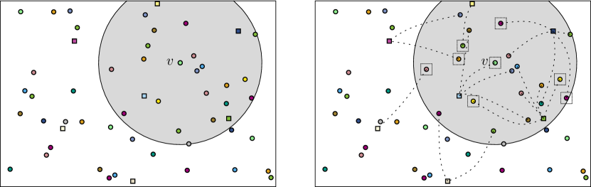
Figure 3: Left: Node $v$ with its broadcasting region in a network with valid coloring; Nodes in the first level MIS are squares. Right: Nodes in $v$’s broadcasting range are connected to their selected leader by a dashed line. Nodes currently active in the second level are surrounded by a square.

Compared to the classical local broadcasting algorithm, we increase the transmission probability by a factor of $\Delta$, thus decreasing the time to successful message transmission by the same factor of $\Delta$ to $\mathcal{O}(\log n)$. This is possible as instead of $\Delta$ only a constant number of nodes try to transmit. Based on this result we can bound the runtime of our algorithm, starting with Algorithm 5.

Lemma 13.

Let $v$ execute Algorithm 5 with leader $w$. Then a) $v$transmits the request message successfully within $\kappa_{1}$ time slots w.h.p.; b) $v$receives its active interval after at most another $\kappa_{1}$ time slots w.h.p.; and c) $t\leq\Delta 2k^{2}\kappa_{2}\in\mathcal{O}(\Delta\log n)$.

Proof.

Part a) is implied directly by Lemma 5. Regarding Part b), it holds that $v$’s leader node $w$ must answer at most $\Delta$ requests. For each request $w$ transmits the node’s answer for $\kappa_{2}$ time slots. Thus $v$ receives its active interval at most $\kappa_{1}+\Delta\kappa_{2}$ time slots after it started transmitting its request. Part c) holds by definition of $\tau(\cdot,\cdot)$. ∎

We shall now argue that each non-leader node succeeds to win a second level MIS in its active interval.

Lemma 14.

Given a node $v$ executing Algorithm 5. Once $t=0$, $v$ wins a second level MIS set within $2k^{2}\kappa_{2}$ time slots.

Proof.

The active interval of $v$ is from $t_{s}=0$ to $t_{e}=2k^{2}\kappa_{2}$. According to Lemma 12, at most $k$ nodes are active in $v$’s broadcasting range at any time (including $v$). As nodes are active for $2k^{2}\kappa_{2}$ consecutive time slots, it holds that during the interval $\{t_{s},\dots,t_{e}\}$ at most $2k-2$ neighbors of $v$ are active as well. With each MIS execution at the second level at least one neighbor gets to be in an independent set, selects a valid color, transmits this color to its neighbors and does not participate in following MIS executions. Thus, after at most $2k-2$ MIS executions $v$ either succeeded in a previous MIS execution, or all active neighbors of $v$ succeeded and thus $v$ must succeed in the next second level MIS execution. ∎

As a final step we show that the final color the nodes select are valid w.h.p.

Lemma 15.

Given a node $v$ entering Algorithm 4. It holds that a) while $v$ transmits its final color no neighbor of $v$ succeeds in a second level MIS w.h.p.; and b) the color $v$ selects is not selected by one of $v$’s neighbors w.h.p.

Proof.

Part a) holds since all neighbors of $v$ that participated in the current second level MIS know the counter value of $v$ w.h.p., and hence do not enter the MIS before $v$ finished transmitting its final color. As the nodes are not synchronized, a node $w$ may have just entered the active interval. In this case, however, the listening phase of $\kappa_{2}$ time slots prevents $w$ from succeeding before it knows the status of all active neighbors. Thus, while $v$ transmits its color, no neighbors of $v$ select their final color (except for first level leaders taking color 0, which does not conflict with the second level coloring). For Part b) observe that the algorithm removes each final color it receives from the set of available colors according to Algorithm 2. Due to Part a) it holds that the colors of all neighbors of $v$ that selected a final color before $v$ were able to transfer the color to $v$ successfully. Thus $v$ selected a color which was not selected by one of its neighbors. ∎

We are now able to prove the main theorem. Note that runtime bounds hold for each node beginning with the node start executing the algorithm.

Proof of Theorem 11.

The number of colors used follows directly from the algorithm. It follows from Lemma 15 and the fact that each node succeeds in an MIS (and hence enters Algorithm 4 and selects a final color), that the final color of each node is valid w.h.p. A simple union bound over all nodes implies that the $\Delta+1$ coloring is valid. The runtime follows as the first level MIS takes $\mathcal{O}(\Delta\log n)$ time slots according to Lemma 10, Algorithm 5 takes another $\mathcal{O}(\Delta\log n)$ slots until starting the active interval, which is of length $\mathcal{O}(\log n)$. ∎

Corollary 16.

Let each node in the network execute the MW-coloring algorithm from [5] followed by Algorithm 2. Then $\mathcal{O}(\Delta\log n)$ time slots after a node started executing the algorithm it has a valid color from $[\Delta]$.

Concurrent Execution of Algorithms: We consider this algorithm isolated from other algorithms that may be executed simultaneously by other nodes (which just woke up, for example). The additional interference introduced by a constant number of different algorithms that are executed simultaneously in the network can be handled simply by reducing the transmission probabilities used in the algorithms by the number of algorithms executed simultaneously.

6 Conclussion

We conclude that the proposed distributed $\Delta+1$ coloring algorithms are simple and very fast. They are based on a simple and well-known randomized $\Delta+1$ coloring algorithm and a color reduction scheme. By carefully balancing the uncertainties due to communication in the physical or SINR model and the uncertainties in the randomized algorithm itself, we are able to guarantee a runtime of $\mathcal{O}(\Delta\log n)$ time slots for all our algorithms. This corresponds to just a few rounds of local broadcasting and outperforms all previous algorithms either by the number of colors required or the running time.

Acknowledgements: We thank Magnús M. Halldórsson for helpful discussions on an early stage of this work, and the German Research Foundation (DFG), which supported this work within the Research Training Group GRK 1194 ”Self-organizing Sensor-Actuator Networks”.

Appendix A Appendix

A.1 Omitted Proofs

Restatement of Lemma 2, which establishes a bound on the sum of transmission probabilities from within each broadcasting region based on the transmission probabilities $p_{1}$ and $p_{2}$ used for communication in the algorithms. See 2

Proof.

Depending on the algorithm, nodes in $v$’s broadcasting range are either transmitting with probability $p_{1}$ or $p_{2}$. It holds that most nodes transmit with probability $p_{1}$ for all algorithms. For the use of probability $p_{2}$ in Algorithm 1 is holds that at most a 5 nodes from within each broadcasting range transmit with probability $p_{1}$, since in a broadcasting range in which more than 5 nodes have the same color, two of them must be neighbors. This would violate the validity of the $4\Delta$ coloring of the network, which is guaranteed by Proposition 8. For Algorithm 2 it holds that at most 90 nodes within $v$’s broadcasting range use $p_{1}$ according to Lemma 12.

Let us now consider both cases jointly, and let $p_{w}$ be the current transmission probability of $w$, which is either $p_{1}$, $p_{2}$ or 0 if $w$ is currently not trying to transmit (e.g. if $c^{t}_{v}\not=i$ in Algorithm 1). Let us now bound the sum of transmission probabilities from within $B_{v}$.

$$\sum_{w\in B_{v},\atop w\text{ transmits}}p_{w} \leq\sum_{w\in B_{v}}p_{1}+\sum_{w\in B_{v},\atop w\text{ transmits with }p_{2}}p_{2}$$

$$\leq\Delta\cdot\frac{1}{2\Delta^{A}}+90\cdot\frac{1}{180}\leq 1,$$

where the last inequality holds since $r_{A}>2r_{B}$ which implies $\Delta\leq\Delta^{A}$. ∎

A.2 Successful Transmission with Constant Probability

In this section, we give a full proof for Theorem 3. The following proof is largely based on the proof of Lemma 4.1 and Theorem 4.2 by Goussevskaia, Moscibroda and Wattenhofer [1]. Before proving the result, let us introduce some additional notation required in this section.

A.2.1 Further definitions

Definitions of the transmission and the broadcasting range are given in Section 2. We shall give more details about the proximity range here. Let us consider an arbitrary node $v$. In accordance with [1], we define the proximity range around $v$ to be $r_{A}=r_{B}\left(3^{3}2^{\alpha}\beta\cdot\left(\frac{\alpha-1}{\alpha-2}\right)\right)^{\frac{1}{\alpha-2}}$, and denote set of nodes within the transmission range of $v$ by $A_{v}$. Let $\chi:=\frac{2\pi}{3\sqrt{3}}\frac{(r_{A}+2r_{B})^{2}}{r_{B}^{2}}$. This is, intuitively speaking, bound on the number of independent broadcasting ranges that can be fit in a disk of radius $r_{A}$.

A.2.2 Full proof of Theorem 3

We shall now prove Theorem 3 (restated in the following). See 3

Proof.

Let us first prove the two major observations that are implied by the fact that the sum of transmission probabilities from within each broadcasting range is bounded by 1. These observations are formulated in the two following claims. The probabilities proven in these claims can be combined with the transmission probability to form the probability that $v$ succeeds in transmitting its message in a given time slot. After proving the claims, we shall show that these probabilities indeed imply a constant success probability of $11/12$.

Claim 17.

The probability $P^{A_{v}}_{\text{none}}$ that $v$ is the only node in the proximity region that transmits a signal in the current time slot is at least $(1/4)^{\chi}$, and thus constant.

Proof of the claim.

Let us consider the probability that any other node in $v$’s proximity region attempts to transmit. Again, let $p_{w}$ be the current transmission probability of $w$, which is either $p_{a}$, $p_{s}$ or 0 if $w$ is currently not trying to transmit.

$$P^{A_{v}}_{\text{none}} \geq\prod_{w\in A_{v}\backslash\{v\}}(1-p_{w})\geq\left(\frac{1}{4}\right)^{\sum_{w\in A_{v}\backslash\{v\}}p_{w}}$$

$$\geq\left(\frac{1}{4}\right)^{\sum_{u\in A_{v}\backslash\{v\},\atop u\text{ independent}}\sum_{w\in B_{u}}p_{w}}$$

$$\geq\left(\frac{1}{4}\right)^{\sum_{u\in A_{v}\backslash\{v\},\atop u\text{ independent}}1}\geq\left(\frac{1}{4}\right)^{\chi},$$

where the second inequality holds due to Fact 3.1 in [1], the third inequality follows by covering the nodes in $A_{v}$ by broadcasting ranges of independent nodes in $A_{v}$. The next inequality is implied by Lemma 2, while the last inequality holds as $\chi$ is (roughly speaking) the number of independent nodes in $A_{v}$. The claim follows from observing that $\chi$ is indeed constant as the number of disks required to cover a (by a constant) larger disk is constant (cf. Fact 3.3 in [1]). ∎

As the proof of the following claim is in parts exactly as already covered in [1], we omit the bound on the interference received from nodes outside of the proximity area of $v$ on nodes in the broadcasting range of $v$.

Claim 18.

The probability $P^{v}_{\text{SINR}}$ that the SINR constraint holds for a given transmission is at least $1/2$.

Proof of the claim.

The proof is based on the concept of rings around the transmitting node $v$. With increasing distance the number of nodes in a ring increases, however, also the effects on nodes in the broadcasting range of $v$ decreases. Based on Lemma 2, the bound on the interference received at an arbitrary node $w$ in $v$’s broadcasting range can be bound by $\frac{P}{4\beta r_{B}^{\alpha}}$ exactly as in [1]. Now, applying the Markov inequality it holds that the probability that the interference is more than twice this level (and thus the SINR constraint is violated) is at most $1/2$. It follows that the SINR constraint holds with probability at least $1/2$. ∎

Combining the probabilities from the previous claims with the transmission probability $p_{v}$, it follows that the probability that $v$ successfully transmits a message to all neighbors in a given time slot is at least $p_{v}\cdot P^{A_{v}}_{\text{none}}\cdot P^{v}_{\text{SINR}}$. As $\lambda:=\left(P^{A_{v}}_{\text{none}}\cdot P^{v}_{\text{SINR}}\right)^{-1}$, the probability for a successful transmission to all neighbors after $\frac{\lambda\ln 12}{p}$ time slots is at least

$$1-\left(1-\frac{p}{\lambda}\right)^{\frac{\lambda\ln 12}{p}}\geq 1-e^{-\ln 12}\geq 1-\frac{1}{12}\geq\frac{11}{12},$$

which concludes the proof. ∎

A.3 Discussion and Future Work

Local Synchronization: Let us briefly discuss the assumptions of our algorithms for the synchronous setting. A wireless network can be synchronized either by using network-wide broadcasts, or by applying synchronization methods such as Timing-sync Protocol for Sensor Networks (TPSN) [29]. Assuming a node with a valid clock within few hops of each node, the network can be synchronized within a few rounds of local broadcasting. Then, the simple synchronous coloring algorithms presented in Section 4 can be used to compute a $\Delta+1$ coloring.

Without knowledge of $\Delta$: If this upper bound on the local density is not known, one must begin with a very low transmission probability and use a so-called slow-start technique to find the correct transmission probability. Current slow-start techniques for local broadcasting require $\mathcal{O}(\Delta\log n+\log^{2}n)$ time slots [2, 3]. Unfortunately, we cannot adapt the slow-start technique to achieve successful message transmission with constant probability as shown for the case with knowledge of $\Delta$ in Section 3.

For the algorithm by Halldórsson and Mitra [2], reducing the runtime by a $\log n$ factor by allowing success with only constant probability (instead of w.h.p.) fails as we cannot guarantee that the so-called fallback occurs with high probability, which is required to keep the sum of local transmission probabilities low. It would be interesting to find an algorithm that achieves message transmission with constant probability without the knowledge of $\Delta$ that improves the runtime bound of $\mathcal{O}(\Delta\log n+\log^{2}n)$. Such an algorithm could generalize the algorithms presented in this work to operate without prior knowledge of $\Delta$.

References

- [1] O. Goussevskaia, T. Moscibroda, and R. Wattenhofer, “Local Broadcasting in the Physical Interference Model,” in Proc. 5th ACM Internat. Workshop on Foundations of Mobile Computing (DialM-POMC’08). ACM, 2008, pp. 35–44.
- [2] M. M. Halldórsson and P. Mitra, “Towards Tight Bounds for Local Broadcasting,” in Proc. 8th ACM Internat. Workshop on Foundations of Mobile Computing (FOMC’12). ACM, 2012.
- [3] D. Yu, Q.-S. Hua, Y. Wang, and F. C. M. Lau, “An Distributed Approximation Algorithm for Local Broadcasting in Unstructured Wireless Networks,” in Proc. 8th Internat. Conf. on Distributed Computing in Sensor Systems (DCOSS’12). IEEE, 2012, pp. 132–139.
- [4] F. Fuchs and D. Wagner, “Local broadcasting with arbitrary transmission power in the SINR model,” in Proc. 21st Internat. Colloq. Structural Inform. and Communication Complexity (SIROCCO’14), ser. Lecture Notes Comput. Sci., M. M. Halldórsson, Ed., vol. 8576. Springer, 2014, pp. 180–193.
- [5] B. Derbel and E.-G. Talbi, “Distributed Node Coloring in the SINR Model,” in Proc. 30th Internat. Conf. on Distributed Computing Systems (ICDCS’10). IEEE, 2010, pp. 708–717.
- [6] F. Fuchs and D. Wagner, “On Local Broadcasting Schedules and CONGEST Algorithms in the SINR Model,” in Proc. 9th Internat. Workshop on Algorithmic Aspects of Wireless Sensor Networks (ALGOSENSORS’13), 2013, pp. 170–184.
- [7] M. R. Garey and D. S. Johnson, Computers and Intractability: A Guide to the Theory of NP-Completeness. W. H. Freeman & Co., 1979.
- [8] T. Moscibroda, R. Wattenhofer, and Y. Weber, “Protocol design beyond graph-based models,” in Proc. of the ACM Workshop on Hot Topics in Networks (HotNets-V), 2006, pp. 25–30.
- [9] L. Barenboim and M. Elkin, Distributed Graph Coloring: Fundamentals and Recent Developments, ser. Synthesis Lectures on Distributed Computing Theory. Morgan & Claypool Publishers, 2013.
- [10] D. Yu, Y. Wang, Q.-S. Hua, and F. C. Lau, “Distributed ( + 1) Coloring in the Physical Model,” Theoret. Comput. Sci., vol. 553, no. 0, pp. 37 – 56, 2014.
- [11] L. Barenboim, M. Elkin, S. Pettie, and J. Schneider, “The locality of distributed symmetry breaking,” in Proc. 53rd Ann. IEEE Symp. Foundations Comput. Sci. (FOCS’12). IEEE, 2012, pp. 321–330.
- [12] J. Schneider and R. Wattenhofer, “A log-star distributed maximal independent set algorithm for growth-bounded graphs,” in Proc. 27th ACM Symp. on Principles of Distributed Computing (PODC’08). ACM, 2008, pp. 35–44.
- [13] N. Linial, “Distributive graph algorithms global solutions from local data,” in Proc. 28th Ann. IEEE Symp. Foundations Comput. Sci. (FOCS’87). IEEE, 1987, pp. 331–335.
- [14] B. Awerbuch, M. Luby, A. Goldberg, and S. A. Plotkin, “Network decomposition and locality in distributed computation,” in Proc. 30th Ann. IEEE Symp. Foundations Comput. Sci. (FOCS’89). IEEE, 1989, pp. 364–369.
- [15] A. Panconesi and A. Srinivasan, “On the complexity of distributed network decomposition,” J. Algorithms, vol. 20, no. 2, pp. 356–374, 1996.
- [16] L. Barenboim, M. Elkin, and F. Kuhn, “Distributed -coloring in linear (in ) time,” SIAM J. Comput., vol. 43, no. 1, pp. 72–95, 2014.
- [17] M. Luby, “Removing randomness in parallel computation without a processor penalty,” in Proc. 29th Ann. IEEE Symp. Foundations Comput. Sci. (FOCS’88). IEEE, 1988, pp. 162–173.
- [18] P. Gupta and P. R. Kumar, “The capacity of wireless networks,” IEEE Trans. on Inform. Theory, vol. 46, no. 2, pp. 388–404, 2000.
- [19] O. Goussevskaia, Y. A. Pignolet, and R. Wattenhofer, “Efficiency of wireless networks: Approximation algorithms for the physical interference model,” Foundations and Trends in Networking, vol. 4, no. 3, November 2010.
- [20] S. Daum, S. Gilbert, F. Kuhn, and C. Newport, “Broadcast in the ad hoc SINR model,” in Proc. 27th Internat. Symp. on Distributed Computing (DISC’13), ser. Lecture Notes Comput. Sci., Y. Afek, Ed. Springer, 2013, vol. 8205, pp. 358–372.
- [21] T. Jurdzinski, D. R. Kowalski, M. Rozanski, and G. Stachowiak, “Distributed randomized broadcasting in wireless networks under the sinr model,” in Proc. 27th Internat. Symp. on Distributed Computing (DISC’13), ser. Lecture Notes Comput. Sci., Y. Afek, Ed., vol. 8205. Springer, 2013, pp. 373–387.
- [22] T. Jurdzinski and D. R. Kowalski, “Distributed Backbone Structure for Algorithms in the SINR Model of Wireless Networks,” in Proc. 26th Internat. Symp. on Distributed Computing (DISC’12), ser. Lecture Notes Comput. Sci. Springer, 2012, pp. 106–120.
- [23] T. Moscibroda and M. Wattenhofer, “Coloring Unstructured Radio Networks,” J. Distr. Comp., vol. 21, no. 4, pp. 271–284, 2008.
- [24] T. Moscibroda and R. Wattenhofer, “Coloring unstructured radio networks,” in Proc. 17th ACM Symp. on Parallelism in Algorithms and Architectures (SPAA’05). ACM, 2005, pp. 39–48.
- [25] J. Bardwell, “Converting signal strength percentage to dbm values,” WildPackets’ White Paper, 2002.
- [26] R. Motwani and P. Raghavan, Randomized algorithms. Chapman & Hall/CRC, 2010.
- [27] M. Luby, “A simple parallel algorithm for the maximal independent set problem,” SIAM J. Comput., vol. 15, no. 4, pp. 1036–1053, 1986.
- [28] J. Schneider and R. Wattenhofer, “Coloring unstructured wireless multi-hop networks,” in Proc. 28th ACM Symp. on Principles of Distributed Computing (PODC’09). ACM, 2009, pp. 210–219.
- [29] S. Ganeriwal, R. Kumar, and M. B. Srivastava, “Timing-sync protocol for sensor networks,” in Proc. 1st Internat. Conf. on Embedded Networked Sensor Systems (SenSys’03). ACM, 2003, pp. 138–149.