Random Preferential Attachment Hypergraphs

Abstract

The random graph model has recently been extended to a random preferential attachment graph model, in order to enable the study of general asymptotic properties in network types that are better represented by the preferential attachment evolution model than by the ordinary (uniform) evolution lodel. Analogously, this paper extends the random hypergraph model to a random preferential attachment hypergraph model. We then analyze the degree distribution of random preferential attachment hypergraphs and show that they possess heavy tail degree distribution properties similar to those of random preferential attachment graphs. However, our results show that the exponent of the degree distribution is sensitive to whether one considers the structure as a hypergraph or as a graph.

Keywords: Random Hypergraphs, Preferential attachment, Social Networks, Degree Distribution.

1 Introduction

Random structures have proved to be an extremely useful concept in many disciplines, including mathematics, physics, economics and communication systems. Examining the typical behavior of random instances of a structure allows us to understand its fundamental properties. The foundations of random graph theory were first laid in a seminal paper by Erdős and Rényi in the late 1950’s [7]. Subsequently, several alternative models for random structures, often suitable for other applications, were suggested. One of the most important alternative models is the preferential attachment model [2], which was found particularly suitable for describing a variety of phenomena in nature, such as the “rich get richer” phenomena, which cannot be adequately simulated by the original Erdős-Rényi model. It has been shown that the preferential attachment model captures some universal properties of real world social networks and complex systems, like heavy tail degree distribution and the “small world” phenomenon [12].

One limitation of graphs is that they only capture dyadic (or binary) relations. In real life, however, many natural, physical and social phenomena involve $k$-ry relations for $k>2$, and therefore can be more accurately represented by hypergraphs than by graphs. For example, collaborations among researchers, as manifested through joint coauthorships of scientific papers, may be better represented by hyperedges and not edges. Figure 1(a) depicts the hypergraph representation for coauthorship relations on four papers: paper 1 authored by $\{a,b,e,f\}$, paper 2 authored by $\{a,c,d,g\}$, paper 3 authored by $\{b,c,d\}$ and paper 4 authored by $\{e,f\}$. Likewise, wireless communication networks [1] or social relations captured by photos that appear in Facebook and other social media also form hyperedges [14]. Affiliation models [10, 13], which are a popular model for social networks, are commonly interpreted as bipartite graphs, where in fact they may sometimes be represented more conveniently as hypergraphs. Figure 1(b) presents the bipartite graph representation of the hypergraph $H$ of Figure 1(a). Sometimes, one can only access the observed graph $G(H)$ of the original hypergraph $H$, that is, only the pairwise relation between players is available (see Figure 1(c)). In some cases this structure may be sufficient for the application at hand, but in many other cases the hypergraph structure is more accurate and informative/

The study of hypergraphs, and in particular random hypergraph models, has its roots in a 1976 paper by Erdős and Bollobas [3], which offers a model analogous to the Erdős-Rényi random graph model [7]. Recently, several interesting properties regarding the evolution of random hypergraphs in this model were studied in [5, 6, 8].

The current paper is motivated by the observation that, just as in the random graph case, the random hypergraph model is not suitable for studying social networks. Our first contribution is in extending the concept of random preferential attachment graphs to random preferential attachment hypergraphs. We believe the this natural model will turn out to be useful in the future study of social networks and other complex systems.

The main technical contribution is that we analyze the degree distribution of random preferential attachment hypergraphs and show that they possess heavy tail degree distribution properties, similar to those of random preferential attachment graphs. However, our results show that the exponent of the degree distribution is sensitive to whether one considers the structure as a hypergraph or as a graph.

As a reference point, we consider the random preferential attachment graph model of Chung and Lu [4]. In that model, starting from an initial graph $G_{0}$, at any time step there occurs an event of one of two possible types: (1) a vertex-arrival event, occuring with probability $p$, where a new vertex joins the network and selects its neighbor among the existing vertices via preferential attachment, or (2) an edge-arrival event, occuring with probability $1-p$, where a new edge joins the network and selects its two endpoints from among the existing vertices via preferential attachment. It is shown in [4] that the degree distribution of the random preferential attachment graph follows a power law, i.e., the probability of a random vertex to be of degree $k$ is proportional to $k^{-\beta}$, with $\beta^{G}=2+\frac{p}{2-p}$. A similar result can be shown in a setting where, at each time step, $d$ edges join the graph instead of only one (in either a vertex event or an edge event)[12]. This result holds even if at each step a random number of edges join the network, so long as the expected number of new edges is $d$ and the variance is bounded.

The model proposed here extends Chung and Lu’s [4] model to support hypergrpahs. That is, the process starts with an initial hypergrpah, and at each time step a random hyperedge joins the network. With probabilty $p$ this new random hyperedge includes a new vertex, and with probabilty $1-p$ it does not. Our model allows the hyperedge sizes to be random (with some restrictions) and the members of each edge are selected randomly according to preferential attachment.

We show that the degree distribution of the resulting hypergraph (as well as the observed graph) follows a power law, but with an exponent $\beta^{H}=2+\frac{p}{\mu-p}$, where $\mu$ is the expected size of an hyperedge.

Our results indicate that one should be careful when studying an observed graph of a general $k$-ry relation. In particular, it makes a difference if the observed graph was generated by a graph or by a hypergraph evolution mechanism, since the two generate observed graphs with different degree distributions.

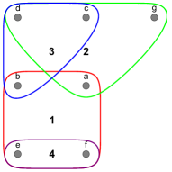
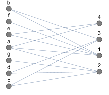
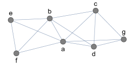
(a)	(b)	(c)

Figure 1: (a) A hypergraph $H$ with 7 vertices and 4 edges. (b) A bipartite graph representation of $H$. (c) The observed graph $G(H)$.

In the next sections we describe in more detail the preferential attachment model of a hypergraph, and then analyze the resulting degree distribution.

2 Preliminaries

Given a set $V$ and a natural $k>1$, let $V^{(k)}$ be the set of all unordered vectors (or multisets) of $k$ elements from $V$. A finite undirected graph $G$ is an ordered pair $(V,E)$ where $V$ is a set of $n$ vertices and $E\subseteq V^{(2)}$ is the set of graph edges (unordered pairs from $V$, including self loops).

A hypergraph $\mathcal{H}$ is an ordered pair $(V,\mathcal{E})$, where $V$ is a set of $n$ vertices and $\mathcal{E}\subseteq\bigcup_{i=2}^{n}V^{(i)}$ is a set of hyperedges connecting the vertices (including self loops). The rank $r({\cal H})$ of a hypergraph ${\cal H}$ is the maximum cardinality of any of the hyperedges in the hypergraph. When all hyperedges have the same cardinality $k$, the hypergraph is said to be $k$-uniform. A graph is thus simply a 2-uniform hypergraph. The degree of a hyperedge $e\in{\cal E}$ is defined to be $\delta(e)=\lvert e\rvert$. The set of all hyperedges that contain the vertex $v$ is denoted $\mathcal{E}(v)=\{e\in\mathcal{E}\mid v\in e\}$. The degree $d(v)$ of a vertex $v$ is the number of hyperedges in ${\cal E}(v)$, i.e., $d(v)=\lvert{\cal E}(v)\rvert$. $\mathcal{H}$ is $d$-regular if every vertex has degree $d$.

In the classical preferential attachment graph model [2], the evolution process starts with an arbitrary finite initial network $G_{0}$, which is usually set to a single vertex with a self loop. Then this initial network evolves in time, with $G_{t}$ denoting the network after time step $t$. In every time step $t$ a new vertex $v$ enters the network. On arrival, the vertex $v$ attaches itself to an existing vertex $u$ chosen at random with probability proportional to $u$’s degree at time $t$, i.e.,

$$\mathbb{P}\left[u\text{ is chosen}\right]~{}=~{}\frac{d_{t}(u)}{\sum_{w\in G_{t}}d_{t}(w)}~{},$$

where $d_{t}(x)$ is the degree of vertex $x$ at time $t$.

3 The nonuniform preferential attachment hypergraph model

Similar to the classical preferential attachment graph model [4], the evolution of the hypergraph occurs along a discrete time axis, with one event occurring at each time step. We consider two types of possible events on the hypergraph at time $t$: (1) a vertex arrival event, which involves adding a new vertex along with a new hyperedge, and a hyperedge arrival event, where a new hyperedge is added.

We consider a nonuniform, random hypergraph where self loops (i.e., multiple appearance of a vertex in a hyperedge) are allowed. We consider self loops as contributing 1 to the vertex degree. Similar to [4], our preferential attachment model, $H(H_{0},p,Y)$, has three parameters:

• A probability $0<p\leq 1$ for vertex arrival events.

• An initial hypergraph $H_{0}$ given at time 0.

• A sequence of random independent integer variables $Y=(Y_{0},Y_{1},Y_{2},\dots)$, for $Y_{i}\geq 2$, which determine the cardinality of the new hyperedge arriving at time $t$.

The process by which the random hypergraph $H(H_{0},p,Y)$ grows in time is as follows.

• We start with the initial hypergraph $H_{0}$ at time 0.

• At time $t>0$, the graph $H_{t}$ is formed from $H_{t-1}$ in the following way:

  • Randomly draw a bit $b$ with probability $p$ for $b=0$.

  • If $b=0$, then add a new vertex $u$ to $V$, select $Y_{t}-1$ vertices from $H_{t-1}$ (possibly with repetitions) independently in proportion to their degrees in $H_{t-1}$, and form a new hyperedge $e$ that includes $u$ and the $Y_{t}-1$ selected vertices.

  • Else, select $Y_{t}$ vertices from $H_{t-1}$ (possibly with repetitions) independently in proportion to their degrees in $H_{t-1}$, and form a new hyperedge $e$ that includes the $Y_{t}$ selected vertices.

Hereafter, we consider an initial $H_{0}$ consisting of a single hyperedge of cardinality $Y_{0}$ over a single vertex (recall that self-loops are considered as contributing 1 to the vertex degree).

4 Degree Distribution Analysis

To ensure convergence of the degree distribution we first need to set some conditions on the distribution of the hyperedge cardinalities. These are somewhat mild conditions that seems to agree with real data (see Fig. 4 in Section 5). Let $Y_{t}$ be independent (not necessarily identical) random variables with constant expectation $\mathbb{E}[Y_{t}]=\mu$ and bounded support s.t. $2<Y_{t}<t^{\frac{1}{3}}$ . Under these conditions we can show the following.

Theorem 4.1.

The degree distribution of a hypergraph $H(H_{0},p,Y)$ where $\mathbb{E}[Y_{t}]=\mu$ follows a power law with $\beta=2+p/(\mu-p)$.

Proof.

We start with properties of $Y_{t}$. Let $S_{t}=\sum_{1}^{t}Y_{t}$, so $\mathbb{E}[S_{t}]=\mu t$ and $S_{t}<t^{\frac{4}{3}}$. The deviation of $S_{t}$ from its expected value can be bounded.

Lemma 4.2.

$\mathbb{P}\left[\lvert S_{t}-\mathbb{E}[S_{t}]\rvert)\geq t^{\frac{2}{3}}\sqrt{2\log t}\right]~{}<~{}O(1/t^{4})$.

Proof.

By Hoeffding’s inequality [9], assuming the random variable $Y_{i}$ satisfies $\mathbb{P}[Y_{i}\in[a_{i},b_{i}]]=1$ for some reals $a_{i}$ and $b_{i}$,

$$\mathbb{P}\left[\lvert S_{t}-\mathbb{E}[S_{t}]\rvert)\geq x\right]~{}\leq~{}2\exp\left(-\frac{2x^{2}}{\sum_{i=1}^{t}(b_{i}-a_{i})^{2}}\right)~{}.$$

Taking $x=t^{\frac{2}{3}}\sqrt{2\log t}$ and noting that $(b_{i}-a_{i})^{2}<t^{\frac{2}{3}}$ and $\sum_{i=1}^{t}(b_{i}-a_{i})^{2}<t^{\frac{4}{3}}$ yields the result. ∎

To bound the degree distribution of a non-uniform random hypergraph we closely follow Chung and Lu’s analysis on preferential attachment graphs [4]. Let $m_{k,t}$ denote the number of vertices of degree $k$ at time $t$. Note that $m_{1,0}=0$ and $m_{0,t}=0$. We derive the recurrence formula for the expected value $\mathbb{E}[m_{k,t}]$. The main observation here is that a vertex has degree $k$ at time $t$ if either it had degree $k$ at time $t-1$ and was not selected into a hyperedge at time $t$, or it had degree $k-1$ at time $t-1$ and was selected into a hyperedge at time $t$. Letting $\mathcal{F}_{t}$ be the $\sigma$-algebra associated with the probability space at time $t$, we have for any $t>0$ and $k>0$:

$$\mathbb{E}[m_{k,t}|\mathcal{F}_{t-1}] = m_{k,t-1}\left(p\mathbb{E}_{Y_{t}}\left[\left(1-\frac{k}{S_{t-1}}\right)^{Y_{t}-1}\right]+(1-p)\mathbb{E}_{Y_{t}}\left[\left(1-\frac{k}{S_{t-1}}\right)^{Y_{t}}\right]\right)$$

$$+m_{k-1,t-1}\left(p\mathbb{E}_{Y_{t}}\left[\left(1-(1-\frac{k-1}{S_{t}}\right)^{Y_{t}-1})\right]\right.$$

$$+\left.(1-p)\mathbb{E}_{Y_{t}}\left[\left(1-\left(1-\frac{k-1}{S_{t}}\right)^{Y_{t}}\right)\right]\right),$$

hence

$$\mathbb{E}[m_{k,t}|\mathcal{F}_{t-1}] = m_{k,t-1}\left(p-\mathbb{E}_{Y_{t}}\left[\frac{(Y_{t}-1)kp}{S_{t}}\right]-O\left(\mathbb{E}_{Y_{t}}\left[\left(\frac{Y_{t}kp}{S_{t}}\right)^{2}\right]\right)\right.$$

$$~{}~{}~{}~{}~{}~{}~{}~{}~{}~{}~{}~{}\left.+1-p-\mathbb{E}_{Y_{t}}\left[\frac{(1-p)Y_{t}k}{S_{t}}\right]-O\left(\mathbb{E}_{Y_{t}}\left[\left(\frac{(1-p)Y_{t}k}{S_{t}}\right)^{2}\right]\right)\right)$$

$$+m_{k-1,t-1}\left(\mathbb{E}_{Y_{t}}\left[\frac{(Y_{t}-1)p(k-1)}{S_{t}}\right]-O\left(\mathbb{E}_{Y_{t}}\left[\left(\frac{Y_{t}pk}{S_{t}}\right)^{2}\right]\right)\right.$$

$$~{}~{}~{}~{}~{}~{}~{}~{}~{}~{}~{}~{}~{}~{}~{}~{}\left.+\mathbb{E}_{Y_{t}}\left[\frac{(1-p)Y_{t}(k-1)}{S_{t}}\right]-O\left(\mathbb{E}_{Y_{t}}\left[\left(\frac{(1-p)k}{S_{t}}\right)^{2}\right]\right)\right)$$

or

$$\mathbb{E}[m_{k,t}|\mathcal{F}_{t-1}]~{}=~{}m_{k,t-1}\left(1-\frac{(\mu-p)k}{S_{t}}+O\left(\frac{k^{2}}{S_{t}^{2}}\right)\right)+m_{k-1,t-1}\left(\frac{(\mu-p)(k-1)}{S_{t}}+O\left(\frac{(k-1)^{2}}{S_{t}^{2}}\right)\right)~{}.$$

Using the bound on $S_{t}$ we can find the expectation $\mathbb{E}[m_{k,t}]$.

$$\mathbb{E}[m_{k,t}] = (1-1/t^{4})\left(\mathbb{E}[m_{k,t-1}]\left(1-\frac{(\mu-p)k}{\mu t\pm t^{\frac{2}{3}}\sqrt{2\log t}}+O\left(\frac{k^{2}}{t^{2}}\right)\right)\right.$$

$$\;\;\;\;\left.+\mathbb{E}[m_{k-1,t-1}]\left(\frac{(\mu-p)(k-1)}{\mu t\pm t^{\frac{2}{3}}\sqrt{2\log t}}+O\left(\frac{k^{2}}{t^{2}}\right)\right)\right)+\frac{1}{t^{4}}\cdot t^{4/3}$$

$$= \mathbb{E}[m_{k,t-1}]\left(1-\frac{(\mu-p)k}{\mu t\pm t^{\frac{2}{3}}\sqrt{2\log t}}+O\left(\frac{k^{2}}{t^{2}}\right)\right)$$

$$\;\;\;\;+\mathbb{E}[m_{k-1,t-1}]\left(\frac{(\mu-p)(k-1)}{\mu t\pm t^{\frac{2}{3}}\sqrt{2\log t}}+O\left(\frac{k^{2}}{t^{2}}\right)\right)+O(1/t^{2})~{}.$$

For $t>0$ and the special case of $k=1$ we have

$$\mathbb{E}[m_{1,t}|\mathcal{F}_{t}]~{}=~{}m_{1,t-1}\left(1-\frac{(\mu-p)k}{S_{t}}+O(\frac{k^{2}}{S_{t}^{2}})\right)+p~{},$$

thus

$$\mathbb{E}[m_{1,t}]~{}=~{}\mathbb{E}[m_{1,t-1}]\left(1-\frac{(\mu-p)k}{\mu t\pm t^{\frac{2}{3}}\sqrt{2\log t}}+O(\frac{k^{2}}{t^{2}})\right)+p+O(1/t^{2})~{}.$$

We use the following lemma of [4].

Lemma 4.3.

[4] Let $(a_{t}),(b_{t}),(c_{t})$ be three sequences such that $a_{t+1}=\left(1-\frac{b_{t}}{t}\right)a_{t}+c_{t}$, $\lim_{t\rightarrow\infty}b_{t}=b>0$ and $\lim_{t\rightarrow\infty}c_{t}=c$. Then $\lim_{t\rightarrow\infty}(a_{t}/t)$ exists and equals $c/(1+b)$.

We show by induction that $\lim_{t\rightarrow\infty}\mathbb{E}[m_{k,t}]/t$ exists and has a limit $M_{k}$ for each $k$. For $k=1$, apply Lemma 4.3 with

$$b_{t}=\frac{\mu-p}{\mu\pm t^{\frac{2}{3}}\sqrt{2\log t}/t}+O(k^{2}/t)~{}~{}\text{ and }~{}~{}c_{t}=p+O(1/t^{2})$$

and hence

$$\lim_{t\rightarrow\infty}b_{t}=\frac{\mu-p}{\mu}~{}~{}\text{ and }~{}~{}\lim_{t\rightarrow\infty}c_{t}=p,$$

to get

$$M_{1}~{}=~{}\lim\limits_{t\rightarrow\infty}\frac{\mathbb{E}[m_{1,t}]}{t}~{}=~{}\frac{\mu p}{2\mu-p}~{}.$$

We now assume that $lim_{t\rightarrow\infty}\mathbb{E}[m_{k-1,t}]/t$ exists and apply Lemma 4.3 again with

$$b_{t}~{}=~{}\frac{(\mu-p)k}{\mu\pm t^{\frac{2}{3}}\sqrt{2\log t}/t}+O\left(\frac{k^{2}}{t}\right)$$

and

$$c_{t}~{}=~{}\frac{\mathbb{E}[m_{k-1,t-1}]}{t}\left(\frac{(\mu-p)(k-1)}{\mu\pm t^{\frac{2}{3}}\sqrt{2\log t}/t}+O\left(\frac{k^{2}}{t}\right)\right)+O\left(\frac{1}{t^{2}}\right)~{}.$$

Then

$$\lim_{t\rightarrow\infty}b_{t}=b=\frac{(\mu-p)k}{\mu}~{}~{}\text{ and }~{}~{}\lim_{t\rightarrow\infty}c_{t}=c=M_{k-1}(\mu-p)(k-1)/\mu~{},$$

and by Lemma 4.3 we get that $lim_{t\rightarrow\infty}\mathbb{E}[m_{k,t}]/t$ exists and satisfies

$$M_{k}~{}=~{}M_{k-1}\frac{(\mu-p)(k-1)}{\mu(1+k(\mu-p)/\mu)}~{}=~{}M_{k-1}\frac{(k-1)}{k+\frac{\mu}{\mu-p}}~{}.$$ (1)

Recall that a power law distribution has the property that $M_{k}\propto k^{-\beta}$ for large $k$.

Now if $M_{k}\propto k^{-\beta}$, then

$$\frac{M_{k}}{M_{k-1}}~{}=~{}\frac{k^{-\beta}}{(k-1)^{-\beta}}~{}=~{}\left(1-\frac{1}{k}\right)^{\beta}~{}=~{}1-\frac{\beta}{k}+O\left(\frac{1}{k^{2}}\right)~{}.$$

By Eq. (1),

$$\frac{M_{k}}{M_{k-1}}~{}=~{}\frac{k-1}{k+\frac{\mu}{\mu-p}}~{}=~{}1-\frac{1+\frac{\mu}{\mu-p}}{k+\frac{\mu}{\mu-p}}~{}=~{}1-\frac{1+\frac{\mu}{\mu-p}}{k}+O\left(\frac{1}{k^{2}}\right)~{},$$

so the exponent $\beta$ of the power law satisfies

$$\beta=1+\frac{\mu}{\mu-p}=2+\frac{p}{\mu-p}~{}.$$

∎

A special case of $H(H_{0},p,Y_{t})$ is when $Y_{t}$ is the constant function $d$ and the hypergraph becomes a $d$-uniform hypergraph denoted as $H(H_{0},p,d)$.

Corollary 4.4.

The degree distribution of a $d$-uniform hypergraph $H(H_{0},p,d)$ follows a power law with $\beta=2+p/(d-p)$.

Figure 2 illustrates the difference in exponents $\beta$ between preferential attachment graphs (i.e., 2-uniform hypergraphs) and 3-uniform hypergraphs as a function of $p$.

In many cases one can only observe the graph $G[H]$ that results of the underlying hypergrph $H$. That is, the set of vertices of $G(H)$ is identical to the set of vertices of $H$ and for every hyperedge $e\in H$ we create edges in $G(H)$ to form a clique between all the vertices in $e$. Now we can prove the following.

Claim 4.5.

The degree distribution of the observed graph $G(H(H_{0},p,d))$ that results from a $d$-uniform hypergraph follows a power law with $\beta=2+p/(d-p)$.

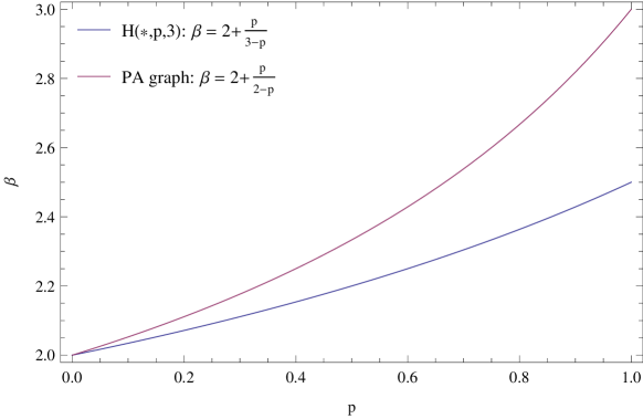
Figure 2: The exponent $\beta$ of a preferential attachment graph and a 3-uniform hypergraph as a function of $p$ (the probability of an edge arrival event). In graphs it is between 2 and 3, whereas in 3-hypergraphs it is between 2 and 2.5.

Note that the expected degree of vertices in $G(H)$ in this case is $d(d-1)/2$. Interestingly, if we generate a new graph $G^{\prime}$ with expected degree $d(d-1)/2$ according to the classical graph preferential attachment model, then its degree distribution will be $\beta^{\prime}=2+p/(2-p)$. Hence the observed degree distribution of $G(H)$ and $G^{\prime}$, $\beta$ and $\beta^{\prime}$ respectively, will be different. On the other hand, it we generate $G^{\prime}$ (using the classical preferential attachment model) so that it agrees with the degree distribution of $G$, then the average degree will be different. This observation is supported by simulation results depicted in Figure 3.

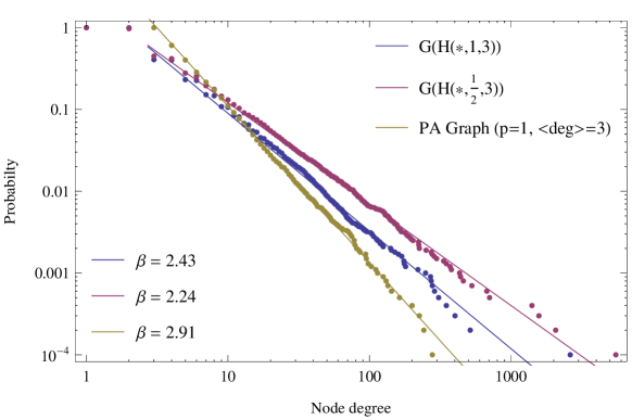
Figure 3: Example of the cumulative degree distribution of three networks with $n=10,000$: (1) A graph $G(H(*,1,3))$ derived from a 3-uniform hypergraph $H(*,1,3)$, (2) A graph $G(H(*,\frac{1}{2},3))$ derived from a 3-uniform hypergraph $H(*,\frac{1}{2},3)$, and (3) A preferential attachment graph with average degree $d(d-1)/2=3$. Graphs derived from hypergraphs have lower exponent, also as a function of $p$.

This discussion seems to indicate that, in some sense, “the blanket (i.e., of the model) is too short” and one should be careful in deciding what is the right model that captures the observed degree distribution, and in particular, if the generative model is of a hypergraph or the classical graph model.

5 Example

To test the above observations empirically, we studied a coauthorship hypergraph of researchers in computer science, extracted from DBLP [11], a dataset recording most of the publications in computer science. This hypergraph consists of hundreds of thousands of vertices (representing authors) and hyperedges (representing papers). Figure 4 shows the degree distribution of hyperedge sizes in DBLP for hyperedges sizes at least 3. The hyperedge size distribution closely fits a power law degree distribution with exponent $\beta=4.66$. This means that the hyperedge size is (with high probabilty) smaller than $m^{1/3}$, where $m$ is the number of papers (hyperedges). For the example of DBLP, where the number of papers is $m=2420879$, the number of authors on a paper (i.e., the hyper-edge size) will be with high probability below $134$.

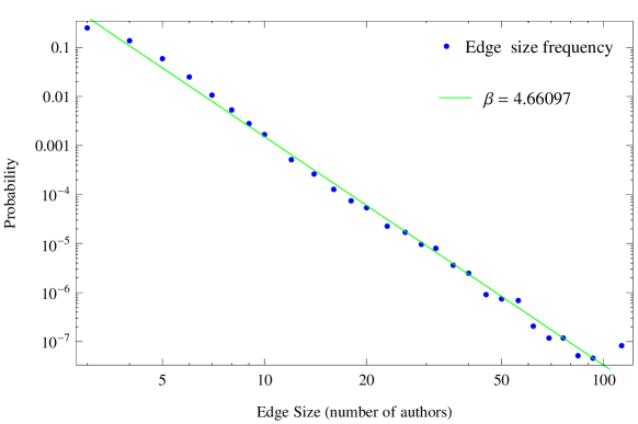
Figure 4: The degree distribution of hyperedge sizes in DBLP for hyperedge sizes at least 3. The distribution closely fits a power law degree distribution with exponent $\beta=4.66$.

References

- [1] Avin, C., Lando, Y., and Lotker, Z. Radio cover time in hyper-graphs. Ad Hoc Networks 12 (2014), 278–290.
- [2] Barabási, A.-L., and Albert, R. Emergence of scaling in random networks. Science 286, 5439 (1999), 509–512.
- [3] Bollobás, B., and Erdös, P. Cliques in random graphs. In Mathematical Proc. Cambridge Philosophical Soc. (1976), vol. 80, Cambridge Univ Press, pp. 419–427.
- [4] Chung, F. R. K., and Lu, L. Complex graphs and networks. No. 107. AMS, 2006.
- [5] Cooper, C., Frieze, A., Molloy, M., and Reed, B. Perfect matchings in random r-regular, s-uniform hypergraphs. Combinatorics, Probability and Computing 5 (1996), 1–14.
- [6] Ellis, D., and Linial, N. On regular hypergraphs of high girth. arXiv preprint arXiv:1302.5090 (2013).
- [7] Erdős, P., and Rényi, A. On the evolution of random graphs. Publ. Math. Inst. Hungar. Acad. Sci 5 (1960), 17–61.
- [8] Ghoshal, G., Zlatić, V., Caldarelli, G., and Newman, M. Random hypergraphs and their applications. Physical Review E 79, 6 (2009), 066118.
- [9] Hoeffding, W. Probability inequalities for sums of bounded random variables. J. Amer. Statistical Assoc. 58, 301 (03 1963), 13–30.
- [10] Lattanzi, S., and Sivakumar, D. Affiliation networks. In Proc. 41st ACM Symp. on Theory of computing (2009), ACM, pp. 427–434.
- [11] Ley, M. Dblp: some lessons learned. Proc. VLDB Endowment 2 (2009).
- [12] Newman, M. Networks: an Introduction. Oxford University Press, 2010.
- [13] Newman, M. E., Watts, D. J., and Strogatz, S. H. Random graph models of social networks. Proc. Nat. Acad. Sci. 99, suppl 1 (2002), 2566–2572.
- [14] Zhang, Z.-K., and Liu, C. A hypergraph model of social tagging networks. J. Statistical Mechanics: Theory and Experiment 2010, 10 (2010), P10005.