Weak values in continuous weak measurement of qubits

Abstract

For continuous weak measurement of qubits, we obtain exact expressions for weak values (WVs) from the post-selection restricted average of measurement outputs, by using both the quantum-trajectory-equation (QTE) and quantum Bayesian approach. The former is applicable to short-time weak measurement, while the latter can relax the measurement strength to finite. We find that even in the “very” weak limit the result can be essentially different from the one originally proposed by Aharonov, Albert and Vaidman (AAV), in a sense that our result incorporates non-perturbative correction which could be important when the AAV’s WV is large. Within the Bayesian framework, we obtain also elegant expressions for finite measurement strength and find that the amplifier’s noise in quantum measurement has no effect on the WVs. In particular, we obtain very useful result for homodyne measurement in circuit-QED system, which allows for measuring the real and imaginary parts of the AAV’s WV by simply tuning the phase of the local oscillator. This advantage can be exploited as efficient state-tomography technique.

I Introduction

The concept of weak value (WV) was introduced by Aharonov, Albert and Vaidman (AAV) in the seminal paper Aha88 and was elaborated with extended discussions Ste89 ; Aha90 . The most interesting and surprising feature of the WV is that it can exceed the range of eigenvalues of the observable. Obviously, the appearance of this nonclassical or strange WV violates our common knowledge that the quantum average must be bounded by the extremum of eigenvalues. Therefore its interpretation has been a subject of confusion Leg89 ; Aha01 . Despite of this, the strange WV has been experimentally confirmed Rit91 ; Wis05 ; DiC13 .

In addition to theoretical curiosity, the concept of WV is very useful to facilitate to resolve and generate quantum paradoxes, such as the Hardy’s paradox Aha02 ; Pay04 , the superluminal transport in optical fiber Bru0304 or in vacuum Aha02a , the momentum-disturbance relationship Wis07 and locally averaged momentum streamlines Hi12 ; Stbg11 in two-slit interferometer, and the more recently proposed quantum Cheshire Cat Aha13 ; Ban14 ; Has14 . Even more, the WV has novel applications in technological aspects, e.g., for weak signal amplification and sensitive estimation of unknown small parameters Kwi08 ; How09 , and for efficient quantum state tomography Lun11 ; Lun12 ; Sa12 .

In AAV’s original work, the WV of spin-$\frac{1}{2}$ particle was proposed as $\langle\sigma^{z}\rangle_{w}={\rm Re}\frac{\langle\psi_{f}|\sigma^{z}|\psi_{i}\rangle}{\langle\psi_{f}|\psi_{i}\rangle}\equiv{\rm Re}(\sigma^{z}_{w})$, where $|\psi_{i}\rangle$ and $|\psi_{f}\rangle$ are the pre- and post-selected states (PPS). Note that the key quantity (we term it in this work as AAV’s WV), $\sigma^{z}_{w}=\frac{\langle\psi_{f}|\sigma^{z}|\psi_{i}\rangle}{\langle\psi_{f}|\psi_{i}\rangle}$, is a complex object. Its interpretation is thus subtle and has caused debates Ste89 ; Aha90 ; Leg89 ; Aha01 . Simpler understanding for WV is from the practical measurement point of view Wis05 ; DiC13 , which is to be termed as measured WV or simply as WV in this work. The measured WV corresponds to a PPS restricted average, say, a sub-ensemble-average of the weak measurement results, with partial data survived from the post-selection.

In most of the existing WV studies, the weak measurement is implemented via a unitary interaction model by two coupled subsystems, i.e., the measured system and the measuring device, while the device is described by a quantum Gaussian probe wavefunction with continuous variables which is subject to extra projective measurement for the “pointer” coordinate or momentum. For this type of model and using a conditional-probability formulation the WV can be re-derived as Dre14 :

$$\langle\sigma^{z}\rangle_{w} = \frac{{}_{f}\langle x\rangle_{i}}{\epsilon}=\int\frac{x}{\epsilon}P_{x}(f;i)dx$$ (1)

$$= {\rm Re}(\sigma^{z}_{w})+O(\epsilon^{2}),$$

where $\epsilon$ is the unitary interaction strength which determines also the average shift of the pointer caused by the system eigenstate. $P_{x}(f;i)$ is the success probability of post-selection with $|\psi_{f}\rangle$, following the $x$-conditioned system state after the weak measurement. Note that this post-selection conditioned average is also the method of data analysis in experiments Wis05 ; DiC13 .

One may note that, differing from the unitary interaction model mentioned above for weak measurements, there exists alternative class of models and real systems, which has been extensively studied for qubit measurement and control, especially in solid-state setup using such as the quantum point contact (QPC) SG97 ; Kor01 ; GM01 , the single electron transistor (SET) Sch98 ; Sch01 , or the homodyne detection in circuit quantum-electrodynamics (cQED) Bla04 ; Wall04 ; Sid12 ; Dev13 ; Sid13 . However, despite particular importance, this type of weak measurement has not yet received much attention in the context of WV studies. Its main difference from the unitary interaction model is that the “device” in this type of measurement scheme is described “classically”, without involving the usual quantum wavefunction description. Instead, this type of weak measurement is characterized by quantum trajectories — the stochastic evolutions of the system state conditioned on the (continuous) measurement outputs, which can be described by quantum-trajectory-equation (QTE) or quantum Bayesian rule. In Ref. Wis02 , applying QTE and using the conditional-probability method, the canonical AAV result of Eq. (1) was recovered for continuous weak measurement of qubit.

In present work, along the line of Ref. Wis02 , we recalculate the WVs for this type of weak measurement. Beyond Eq. (1), we obtain the following better result:

$$\frac{{}_{f}\langle x\rangle_{i}}{\epsilon}=\frac{{\rm Re}(\sigma^{z}_{w})}{1+g(|\sigma^{z}_{w}|^{2}-1)}\,.$$ (2)

Similar as in Eq. (1), the scaling parameter $\epsilon$ in this expression is the shift of the average output current caused by the basis state of the qubit. Notably, in the denominator, $g$ characterizes the measurement strength and takes a simple form $g=\gamma dt$ with $\gamma$ the measurement rate and $dt$ the measurement time.

Remarkable modification of Eq. (2) over Eq. (1) is the “partial”-summation-type term in the denominator. Actually, as long as the expansion $e^{-2g}\simeq 1-2g$ holds to be valid, Eq. (2) is the exact result of the WV. This conclusion can be proved by calculating ${}_{f}\langle x\rangle_{i}$ via the quantum Bayesian rule, which does not restrict the measurement strength to weak limit. We will see that the exact WV result for arbitrary measurement strength corresponds to a simple replacement $g\rightarrow{\cal G}=(1-e^{-2g})/2$ in Eq. (2), while the measurement strength reads $g=\gamma t_{m}$, with $t_{m}$ now a finite time of measurement.

The non-perturbative correction in Eq. (2) cannot be neglected when $\sigma^{z}_{w}$ is large and should be taken into account in the various applications of WVs. For instance, in the context of WV amplifications, it has been pointed out that some “nonlinear” correction to the linear result of AAV WV would set an upper bound for the amplification coefficient, based on similar results obtained within the framework of the unitary interaction model of weak measurements Wu11a ; Wu11b ; Tana11 ; Naka12 ; Sus12 ; Kof12 . As a first and simple remark, our present work differs from those in that we consider different type of weak measurement, which allows for employing different formulations to obtain non-perturbative and exact WV expressions for the measurement of qubits under consideration, in particular obtaining useful result for the solid-state superconducting circuit-QED setup.

The remaining part of this work is organized as follows. In Sec. II, we complete all the formal aspects of calculating the WVs for the continuous weak measurement of solid-state qubits. In Sec. III we specify the study to solid-state circuit-QED setup to carry out useful result which allows for direct measurement of the real and imaginary parts of the AAV WV, by simply tuning the local oscillator’s phase in the homodyne measurement. In Sec. IV we summarize the work with brief remarks.

II Weak values of qubit measurements

II.1 Continuous Measurement of Qubit

There are several experimentally accessible systems for continuous weak measurement of qubits, including for instance the solid-state charge qubit measured by quantum-point-contact or single-electron-transistor SG97 ; Kor01 ; GM01 ; Sch98 ; Sch01 , and the superconducting qubit in circuit-QED Bla04 ; Wall04 measured via the cavity-field homodyne detection Sid12 ; Dev13 ; Sid13 . Under reasonable simplifications, all these setups can be commonly described as follows. First, the qubit Hamiltonian is reduced to a two-state model $H_{q}=\frac{\Delta}{2}\sigma^{z}$, where $\sigma^{z}=|1\rangle\langle 1|-|2\rangle\langle 2|$ and $\Delta=E_{1}-E_{2}$. Second, the measurement principle is based on the distinct stationary current in the detector, $\bar{I}_{1,2}$, which is associated with the qubit state $|1\rangle$ or $|2\rangle$. Moreover, of particular interest is continuous weak measurement for a superposition state $|\psi_{i}\rangle=\alpha|1\rangle+\beta|2\rangle$. In this case, the output current can be expressed in general as $I(t)=I_{0}+\frac{\Delta I}{2}\langle\sigma^{z}\rangle+\xi_{I}(t)$, where $I_{0}=(\bar{I}_{1}+\bar{I}_{2})/2$ and $\Delta I=|\bar{I}_{1}-\bar{I}_{2}|$. The last term obeys the statistics of white noise, with ensemble average ${\rm E}[\xi_{I}(t)\xi_{I}(t^{\prime})]=\frac{S_{0}}{2}\delta(t-t^{\prime})$, where $S_{0}$ is the spectral density of the output current. In this work, we would like to adopt a reduced description, by denoting the measurement output as $J(t)=\frac{I(t)-I_{0}}{\sqrt{S_{0}/2}}$. Then we have $J(t)=2\sqrt{\gamma}\langle\sigma^{z}\rangle+\xi(t)$, where $\gamma=\frac{(\Delta I)^{2}}{8S_{0}}$ and ${\rm E}[\xi(t)\xi(t^{\prime})]=\delta(t-t^{\prime})$.

II.1.1 QTE Approach

Conditioned on the continuous outcomes of measurement given above, the qubit state evolution (in the rotating frame with respect to $H_{q}$) is governed by the following Itô-type quantum trajectory equation (QTE) GM01

$$d\rho=\gamma\mathcal{D}[\sigma^{z}]\rho\,dt+\sqrt{\gamma}\mathcal{H}[\sigma^{z}]\rho\,dW(t)\,.$$ (3)

The super-operators are defined as $\mathcal{D}[A]\rho=A\rho A^{\dagger}-\frac{1}{2}\{A^{\dagger}A,\rho\}$, and $\mathcal{H}[A]\rho=A\rho+\rho A^{\dagger}-\mathrm{Tr}[(A+A^{\dagger})\rho]\rho$. The Wiener increment is formally defined by $dW(t)=\xi(t)\,dt$, in experiment which should be extracted from the output current. Then, after a short-time ($dt$) measurement, the state is updated as $\tilde{\rho}(t+dt)=\rho(t)+d\rho(t)$, in the qubit basis which reads

$$\tilde{\rho}_{11}=\rho_{11}+2\sqrt{\gamma}(1-\langle\sigma^{z}\rangle)\rho_{11}\,dW\,,$$ (4a)

$$\tilde{\rho}_{22}=\rho_{22}-2\sqrt{\gamma}(1+\langle\sigma^{z}\rangle)\rho_{22}\,dW\,,$$ (4b)

$$\tilde{\rho}_{12}=\rho_{12}-2\rho_{12}(\gamma\,dt+\sqrt{\gamma}\langle\sigma^{z}\rangle\,dW)\,,$$ (4c)

where $\langle\sigma^{z}\rangle={\rm Tr}[\sigma^{z}\rho(t)]=\rho_{11}-\rho_{22}$. Below we compare this result with the one from the quantum Bayesian approach.

II.1.2 Quantum-Bayesian Approach

The quantum Bayesian approach, originally proposed by Korotkov Kor99 , is based on the well-known Bayes formula in Probability Theory together with a quantum purity consideration. The former is utilized to determine the diagonal elements while the latter is for determination of the off-diagonal ones. In quite compact form, the quantum Bayesian approach updates the qubit state from $\rho$ to $\tilde{\rho}$ according to the following rule:

$$\tilde{\rho}_{11}=\rho_{11}P_{1}(x)/\mathcal{N}(x),~{}~{}~{}\tilde{\rho}_{22}=\rho_{22}P_{2}(x)/\mathcal{N}(x),$$

$$\tilde{\rho}_{12}=\rho_{12}\sqrt{P_{1}(x)P_{2}(x)}/\mathcal{N}(x)\,.$$ (5)

In these formulas, associated with the qubit state $|j\rangle$ ($j=1,2$), $P_{j}(x)$ is the priori probability distribution “knowledge” for the stochastic outputs “$x$”. $\mathcal{N}(x)=\rho_{11}P_{1}(x)+\rho_{22}P_{2}(x)$ is a normalization factor. Note that the last rule (for off-diagonal element) is from a purity consideration. About the distribution “knowledge”, in most cases, the integrated output (denoted here by the stochastic variable “$x$”) satisfies a Gaussian statistics:

$$P_{j}(x)=\frac{1}{\sqrt{2\pi D}}\exp\left[-\frac{(x-\bar{x}_{j})^{2}}{2D}\right]\,,$$ (6)

where $\bar{x}_{1(2)}=\pm\epsilon$ denotes the average output corresponding to qubit state $|1(2)\rangle$, and $D$ is the distribution variance.

As a more special case, let us consider a short-time measurement over $dt$. The measurement result (stochastic “$x$”) simply reads $x=J(t)dt=2\sqrt{\gamma}\langle\sigma^{z}\rangle\,dt+dW(t)$. From this, we can identify $\epsilon=2\sqrt{\gamma}dt$ and $D=dt$. Viewing the small parameters $\epsilon$, $dt$ and $x$, we first expand the exponential functions in the Bayesian formulas to obtain

$$\tilde{\rho}_{11}=\rho_{11}\left(1+\frac{\epsilon x}{D}\right)\left(1+\frac{\epsilon x}{D}\langle\sigma^{z}\rangle\right)^{-1}\,,$$ (7a)

$$\tilde{\rho}_{22}=\rho_{22}\left(1-\frac{\epsilon x}{D}\right)\left(1+\frac{\epsilon x}{D}\langle\sigma^{z}\rangle\right)^{-1}\,,$$ (7b)

$$\tilde{\rho}_{12}=\rho_{12}\left[1+\frac{1}{4}(\frac{\epsilon x}{2D})^{4}\right]\left(1+\frac{\epsilon x}{D}\right)^{-1}\,.$$ (7c)

Performing further expansion up to the second-order of $\epsilon$ and $x$, one can prove their equivalence to Eq. (3) or (4) as follows. Actually, using the Bayesian expansion and applying the calculus $\dot{\rho}_{ij}(t)=[\tilde{\rho}_{ij}(t+\frac{dt}{2})-\tilde{\rho}_{ij}(t-\frac{dt}{2})]/dt$, we obtain for instance $\dot{\rho}_{11}(t)=-\dot{\rho}_{22}(t)=(2\epsilon x/D)\rho_{11}(t)\rho_{22}(t)$, which gives

$$\dot{\rho}_{11}=-\dot{\rho}_{22}=8\gamma\langle\sigma^{z}\rangle\rho_{11}\rho_{22}+4\sqrt{\gamma}\rho_{11}\rho_{22}\xi(t)\,.$$ (8)

Similarly, for the off-diagonal element, we have

$$\dot{\rho}_{12}=-4\gamma\langle\sigma^{z}\rangle^{2}\rho_{12}-2\sqrt{\gamma}\langle\sigma^{z}\rangle\rho_{12}\xi(t)\,.$$ (9)

We may find that these two equations differ from the QTE (3) or (4). Indeed, using the Bayesian rule in this manner, we obtain the Stratonovich-type QTE, but not the Itô-type Kor01 . To obtain the QTE of the Itô-type, one needs to add a term $({\cal F}/2)(d{\cal F}/d\rho_{ij})$ to each $\dot{\rho}_{ij}$, where ${\cal F}$ is the factor before $\xi(t)$ in each equation GM01 . Applying this conversion rule, one obtains

$$\dot{\rho}_{11}=-\dot{\rho}_{22}=4\sqrt{\gamma}\rho_{11}\rho_{22}\xi(t)\,,$$ (10a)

$$\dot{\rho}_{12}=-2\gamma\rho_{12}-2\sqrt{\gamma}\langle\sigma^{z}\rangle\rho_{12}\xi(t)\,.$$ (10b)

This result is the same of Eq. (3) or (4).

Below we make more comparisons. Inserting the above Bayesian expansion into the Itô calculus $\dot{\rho}_{ij}(t)=[\tilde{\rho}_{ij}(t+dt)-\rho_{ij}(t)]/dt$, one can obtain the Itô-type QTE under the Milstein algorithm KP , for which we exemplify

$$d\rho_{11}=4\sqrt{\gamma}\rho_{11}\rho_{22}\,dW - 8\gamma\rho_{11}\rho_{22}(\rho_{11}-\rho_{22})$$ (11)

$$\times\,[(dW)^{2}-dt]\,.$$

Note that this result differs from $d\rho_{11}=4\sqrt{\gamma}\rho_{11}\rho_{22}dW$, which corresponds to the so-called Euler algorithm KP .

Alternatively, if we only keep $dt$ and $dW$ as small parameters in the Bayesian expansions and use the calculus $\dot{\rho}_{ij}(t)=[\tilde{\rho}_{ij}(t+dt)-\rho_{ij}(t)]/dt$, we find that expansion up to the first order of $dt$ and $dW$ corresponds to the Stratonovich-type QTE. However, if keeping terms in the expansion up to $(dW)^{2}$, one arrives to the Itô-type QTE under the Milstein algorithm. This observation tells us that, in order to make the result from the quantum Bayesian rule be fully identical to that given by the Itô-type QTE, one should first make the expansion of the Baysian formula up to $(dW)^{2}$, then set $(dW)^{2}=dt$.

II.2 Weak Values

II.2.1 QTE Approach

The post-selection restricted average can be calculated using the following conditional-probability method:

$$_{f}\langle x\rangle_{i}=\frac{\int dxxP_{i}(x)P_{x}(f)}{\int dxP_{i}(x)P_{x}(f)}\,$$ (12)

where $x$ stands for the stochastic outcome of the weak measurement, with probability $P_{i}(x)$ determined by the qubit state $|\psi_{i}\rangle$. Assuming $|\psi_{i}\rangle=\alpha|1\rangle+\beta|2\rangle$, we have $P_{i}(x)=|\alpha|^{2}P_{1}(x)+|\beta|^{2}P_{2}(x)$, where $P_{1(2)}(x)$ is the priori probability corresponding qubit state $|1(2)\rangle$. $P_{x}(f)$ is the success probability of the post-selection by state $|\psi_{f}\rangle$, following the measurement outcome $x$. As explained above for the continuous measurement of qubit, the output current can be expressed as $J(t)=2\sqrt{\gamma}\langle\sigma^{z}\rangle+\xi(t)$. For time interval $dt$, the output charge (integrated current) is $x=J(t)dt$, and the qubit state is updated via Eq. (3) or (4) by inserting $dW=x-2\sqrt{\gamma}\langle\sigma^{z}\rangle dt$. Then, the success probability of post-selection is $P_{x}(f)=\langle\psi_{f}|\tilde{\rho}(t+dt)|\psi_{f}\rangle$. More explicitly, we have

$$P_{x}(f)=P\,\left\{1+\gamma dt(|\sigma^{z}_{w}|^{2}-1)\right.$$

$$\left.~{}~{}~{}~{}~{}~{}~{}+2\sqrt{\gamma}[{\rm Re}(\sigma^{z}_{w})-\langle\sigma^{z}\rangle]dW\right\}\,,$$ (13)

where $P=|\langle\psi_{f}|\psi_{i}\rangle|^{2}$ and $\sigma^{z}_{w}=\langle\psi_{f}|\sigma^{z}|\psi_{i}\rangle/\langle\psi_{f}|\psi_{i}\rangle$, as defined in Sec. I (Introduction). Straightforwardly, we evaluate the numerator of Eq. (12) as

$$M_{1}=P\{[1+4\gamma dt\langle\sigma^{z}\rangle({\rm Re}(\sigma^{z}_{w})-\langle\sigma^{z}\rangle)](|\alpha|^{2}\bar{x}_{1}+|\beta|^{2}\bar{x}_{2})$$

$$+2\sqrt{\gamma}({\rm Re}(\sigma^{z}_{w})-\langle\sigma^{z}\rangle)[|\alpha|^{2}(D+\bar{x}_{1}^{2})+|\beta|^{2}(D+\bar{x}_{2}^{2})]\}\,,$$

and the denominator as

$$M_{2} = P[1+\gamma dt(|\sigma^{z}_{w}|^{2}-1)-4\gamma\langle\sigma^{z}\rangle dt({\rm Re}(\sigma^{z}_{w})-\langle\sigma^{z}\rangle)$$ (15)

$$+2\sqrt{\gamma}({\rm Re}(\sigma^{z}_{w})-\langle\sigma^{z}\rangle)(|\alpha|^{2}\bar{x}_{1}+|\beta|^{2}\bar{x}_{2})]\,.$$

Accounting for $|\alpha|^{2}+|\beta|^{2}=1$, $|\alpha|^{2}-|\beta|^{2}=\langle\sigma^{z}\rangle$ and $\bar{x}_{1,2}=\pm 2\sqrt{\gamma}dt\equiv\pm\epsilon$, the WV takes then a very compact form as

$$\frac{{}_{f}\langle x\rangle_{i}}{\epsilon}=\frac{{\rm Re}(\sigma^{z}_{w})}{1+g(|\sigma^{z}_{w}|^{2}-1)}\,.$$ (16)

Here, we have denoted $g=\gamma dt$, which characterizes well the measurement strength. This result differs from the canonical AAV WV, ${}_{f}\langle x\rangle_{i}/\epsilon={\rm Re}(\sigma^{z}_{w})$, by a “partial”-summation-type correction in the denominator. However, as we will see in the following, as long as the expansion $e^{-2g}\simeq 1-2g$ holds, Eq. (16) is non-perturbative and exact. As shown in Fig. 1, even in the weak measurement limit (short time $dt$ or small $g$), the role of this correction could be essential when $\sigma^{z}_{w}$ is large. This implies that in the various WV applications such as weak signal amplification, the non-perturbative correction in the denominator of Eq. (16) should be taken into account Wu11a ; Wu11b ; Tana11 ; Naka12 ; Sus12 ; Kof12 .

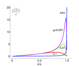
Figure 1: (color online) Non-perturbative correction of Eq. (16) to the canonical AAV WV (blue line). In this plot, we specify the initial state as $|\psi_{i}\rangle=\frac{1}{\sqrt{2}}(|1\rangle+|2\rangle)$ and the post-selection state as $|\psi_{f}\rangle=[(\cos\frac{\theta}{2}+\sin\frac{\theta}{2})|1\rangle+(\cos\frac{\theta}{2}-\sin\frac{\theta}{2})|2\rangle]/\sqrt{2}$, which result in the AAV WV $\sigma^{z}_{w}=\tan(\theta/2)$. We wee that, in contrast to the AAV WV, a different trend appears in the large $\sigma^{z}_{w}$ regime.

II.2.2 Bayesian Approach

Applying the quantum Bayesian rule we first calculate the post-selection probability, $P_{x}(f)={\rm Tr}[\rho_{f}\tilde{\rho}(x)]$, where $\rho_{f}=|\psi_{f}\rangle\langle\psi_{f}|$ is the post-selection state and $\tilde{\rho}(x)$ the updated state from Eq. (II.1.2). The result simply reads

$$P_{x}(f) = \left[\rho_{f11}\rho_{11}P_{1}(x)+\rho_{f22}\rho_{22}P_{2}(x)\right]$$ (17)

$$+2{\rm Re}(\rho_{f12}^{*}\rho_{12})\sqrt{P_{1}(x)P_{2}(x)}\,.$$

$\rho_{ij}$ are the elements of the density matrix of the initial state $\rho=|\psi_{i}\rangle\langle\psi_{i}|$, which gives also the distribution function $P_{i}(x)$ in Eq. (12) as $P_{i}(x)=\rho_{11}P_{1}(x)+\rho_{22}P_{2}(x)$. Straightforwardly, after completing a number of Gaussian integrals, the WV defined by Eq. (12) is obtained as ${}_{f}\langle x\rangle_{i}=M_{1}/M_{2}$, with $M_{1}$ and $M_{2}$ given by

$$M_{1}=(\rho_{f11}\rho_{11}\bar{x}_{1}+\rho_{f22}\rho_{22}\bar{x}_{2})+(\bar{x}_{1}+\bar{x}_{2})$$

$$~{}~{}\times{\rm Re}(\rho_{f12}^{*}\rho_{12})\exp\left[-(\bar{x}_{1}-\bar{x}_{2})^{2}/(8D)\right]\,,$$ (18a)

$$M_{2} = (\rho_{f11}\rho_{11}+\rho_{f22}\rho_{22})+2\,{\rm Re}(\rho_{f12}^{*}\rho_{12})$$ (18b)

$$\times\,\exp\left[-(\bar{x}_{1}-\bar{x}_{2})^{2}/(8D)\right]\,.$$

Since the Bayesian rule works for finite strength measurement, this result is then valid in general.

To be more specific, let us consider an initial state $|\psi_{i}\rangle=\frac{1}{\sqrt{2}}(|1\rangle+|2\rangle)$ and parameterize the post-selection state $|\psi_{f}\rangle=d_{1}|1\rangle+d_{2}|2\rangle$ with polar angle $\theta$ as $d_{1}=(\cos\frac{\theta}{2}+\sin\frac{\theta}{2})/\sqrt{2}$ and $d_{2}=(\cos\frac{\theta}{2}-\sin\frac{\theta}{2})/\sqrt{2}$. Substituting the two states into Eq. (18), we obtain

$$_{f}\langle x\rangle_{i}=\frac{\bar{x}_{1}+\bar{x}_{2}}{2}+\frac{\sin\theta}{1+G\cos\theta}\left(\frac{\bar{x}_{1}-\bar{x}_{2}}{2}\right)\,,$$ (19)

where $G=\exp[-(\bar{x}_{1}-\bar{x}_{2})^{2}/(8D)]$. Similar as Eq. (18), this result is valid for arbitrary strength of measurement.

Now consider the limit of weak measurement based on this result. If we take first the limit $G\rightarrow 1$, we find that the WV can diverge when $\theta\rightarrow\pi$, like the AAV WV, in present case which reads $\sigma^{z}_{w}=\tan(\theta/2)$. This limiting order corresponds also to taking first the limit $g=\gamma dt\rightarrow 0$ in the denominator of Eq. (16), then altering the post-selection to get divergent WV. However, for any real measurement, the measurement strength must be nonzero, which results in ${}_{f}\langle x\rangle_{i}/\epsilon$ behaving as shown in Fig. 1. The turnover behavior implies an existence of optimal post-selection state which maximizes the WV, and vanishing WV when the AAV WV diverges. The latter corresponds to $G\neq 1$ and $\theta\rightarrow\pi$ in Eq. (19).

Moreover, it is desirable to recast the general WV result Eq. (18) into more compact form, like Eq. (16) in the weak measurement limit. In the Bayesian result, let us identify $\bar{x}_{1,2}=\pm 2\sqrt{\gamma}t_{m}=\pm\epsilon$ and $D=t_{m}$, where $t_{m}$ is the finite measurement time. Substituting these into Eq. (18), after some algebra we get

$$\frac{{}_{f}\langle x\rangle_{i}}{\epsilon}=\frac{{\rm Re}(\sigma^{z}_{w})}{1+{\cal G}\,(|\sigma^{z}_{w}|^{2}-1)}\,.$$ (20)

Corresponding to $g=\gamma dt$ in Eq. (16), the counterpart ${\cal G}$ in this result has been generalized to ${\cal G}=(1-e^{-2g})/2$ with $g=\gamma t_{m}$. Obviously, both results are identical for short time limit. This proves also that the QTE result of WV is exact in the weak measurement limit, having not lost anything in the “partial”-summation-type form of Eq. (16).

II.2.3 Noisy Amplification

For many realistic measurements such as in circuit-QED (to be addressed in Sec. III), the weak output signal $x$ must be amplified properly. As a simplified description, the principle of a linear amplifier can be modeled by a second-tier of output voltage as $v_{x}=v_{0}+xR$, where $R$ is the amplification coefficient and $v_{0}$ denotes a reference voltage. In addition to this one-to-one correspondence, the amplifier will inevitably introduce extra noise. Without loss of generality, we assume that the noise is Gaussian. Then, the output voltage $\tilde{v}$ satisfies $P_{x}(\tilde{v})=(2\pi\tilde{\sigma}^{2})^{-1/2}\exp[-\frac{(\tilde{v}-v_{x})^{2}}{2\tilde{\sigma}^{2}}]$. Viewing the relation between $v_{x}$ and $x$, we may reexpress this distribution alternatively as

$$P_{x}(v)=\frac{1}{\sqrt{2\pi\sigma^{2}}}\exp\left[-\frac{(v-x)^{2}}{2\sigma^{2}}\right]\,,$$ (21)

where we have re-defined $\sigma=\tilde{\sigma}/R$ and $v=(\tilde{v}-v_{0})/R$.

Now we analyze the consequence of the amplifier’s noise. Let us consider first how the initial probability of the first-tier output, $P_{i}(x)=\rho_{11}P_{1}(x)+\rho_{22}P_{2}(x)$, should be modified from the amplified signal $\tilde{v}$ (or the re-scaled $v$). This can be done by using the classical Bayes formula:

$$P_{v}(x)=\frac{P_{i}(x)P_{x}(v)}{\int dxP_{i}(x)P_{x}(v)}\,.$$ (22)

This distribution tells us that, for a given amplified signal $v$, there are many possible $x$. Therefore, the $v$-conditioned qubit state should be

$$\tilde{\rho}_{v}=\int dx\tilde{\rho}_{x}P_{v}(x)\,,$$ (23)

where $\tilde{\rho}_{x}$ is the qubit state conditioned on $x$, in general which is given by the quantum Bayesian rule of Eq. (II.1.2). More explicitly, we have

$$\tilde{\rho}_{v,11}=\rho_{11}{\cal B}_{1}(v)/{\cal N}_{v}\,,$$ (24a)

$$\tilde{\rho}_{v,22}=\rho_{22}{\cal B}_{2}(v)/{\cal N}_{v}\,,$$ (24b)

$$\tilde{\rho}_{v,12}=\rho_{12}{\cal B}_{3}(v)/{\cal N}_{v}\,.$$ (24c)

Here, for the sake of brevity, we have introduced ${\cal B}_{1,2}(v)=e^{-\frac{(v-\bar{x}_{1,2})^{2}}{2(D+\sigma^{2})}}$, ${\cal B}_{3}(v)=e^{-\frac{(\Delta\bar{x})^{2}}{8D}}e^{-\frac{(v-\bar{x}_{0})^{2}}{2(D+\sigma^{2})}}$ and ${\cal N}_{v}=\rho_{11}{\cal B}_{1}(v)+\rho_{22}{\cal B}_{2}(v)$, where $\Delta\bar{x}=|\bar{x}_{1}-\bar{x}_{2}|$ and $\bar{x}_{0}=(\bar{x}_{1}+\bar{x}_{2})/2$.

Similar as using Eq. (12), we can calculate now the “noisy” WV by means of

$${}_{f}\langle x\rangle_{i}=\frac{\int dv\,v\,P_{i}(v)P_{v}(f)}{\int dv\,P_{i}(v)P_{v}(f)}\,,$$ (25)

where $P_{i}(v)$ is the probability distribution of the second-tier result “$v$” which is given by

$$P_{i}(v)=\int dxP_{i}(x)P_{x}(v)=\frac{\rho_{11}{\cal B}_{1}(v)+\rho_{22}{\cal B}_{2}(v)}{\sqrt{2\pi(\tilde{\sigma}^{2}+DR^{2})}}\,,$$ (26)

and the post-selection probability reads

$$P_{v}(f)=\rho_{f11}\tilde{\rho}_{v,11}+\rho_{f22}\tilde{\rho}_{v,22}+2\,{\rm Re}(\rho_{f12}\tilde{\rho}_{v,21})\,.$$ (27)

In this way we obtain the result of WV defined from the “polluted” data, after noisy amplification. However, being of some surprise is that we find the same result of Eq. (18). This means that the WV is free from the amplifier’s noise. We may understand this result by the fact that the noisy amplification of the second-tier does affect the distribution width of the outputs, but does not affect their average even in the presence of post-selection.

The extra noise introduced in the amplification process is a sort of non-ideality to reduce the quantum efficiency of measurement. One may expect and actually can prove that other sources of non-ideality owing to quantum information loss does not affect the WV as well. Desirably, the feature that the WV is free from amplifier’s noise and other sources of non-ideality (quantum information loss) can benefit the measurement and applications of the WVs.

III Weak values in Circuit-QED

In this section we specify the WV study carried out above to the solid-state circuit-QED (cQED) system for two reasons. First, the cQED system is one of the most promising solid-state architectures for quantum information processing Bla04 ; Wall04 and excellent platform for quantum measurement and control studies Sid12 ; Dev13 ; Sid13 . Second, this is to-date the most experimentally accessible solid-state system where the continuous weak measurement of the type considered in Sec. II has been realized Sid12 ; Dev13 ; Sid13 . In particular, we will obtain even more useful result than Eq. (16) in that it allows for direct measurement of the full AAV WV, thus for efficient method of qubit state tomography in this important system.

III.1 QTE Approach

Under reasonable approximations, the cQED system is well described by the Jaynes-Cummings Hamiltonian Bla04 . Moreover, in dispersive regime, by performing a qubit-state-dependent displacement transformation (called also “polaron” transformation), it is possible to eliminate the cavity degrees of freedom to get a transformed QTE for the qubit state alone under continuous homodyne measurements Gam08 :

$$\dot{\rho}=-i\frac{\tilde{\omega}_{q}+B(t)}{2}[\sigma^{z},\rho]+\frac{\Gamma_{d}(t)}{2}\mathcal{D}[\sigma^{z}]\rho$$

$$-\sqrt{\Gamma_{ci}(t)}\mathcal{M}[\sigma^{z}]\rho\xi(t)+i\frac{\sqrt{\Gamma_{ba}(t)}}{2}[\sigma^{z},\rho]\xi(t)\,.$$

Here, $\tilde{\omega}_{q}=\omega_{q}+\chi$ is the renormalized qubit energy owing to a dispersive shift $\chi$ to the bare energy $\omega_{q}$; $B(t)=2\chi\mathrm{Re}[\alpha_{1}(t)\alpha^{*}_{2}(t)]$ is a generalized dynamic ac-Stark shift, with $\alpha_{1}(t)$ and $\alpha_{2}(t)$ the cavity fields associated with the qubit states $|1\rangle$ and $|2\rangle$, respectively. In addition to the Lindblad term, a new superoperator is introduced here by $\mathcal{M}[\sigma^{z}]\rho\equiv(\sigma^{z}\rho+\rho\sigma^{z})/2-\langle\sigma^{z}\rangle\rho$, with $\langle\sigma^{z}\rangle={\rm Tr}[\sigma^{z}\rho]$. Also,

$$\Gamma_{d}(t)=2\chi\mathrm{Im}[\alpha_{1}(t)\alpha^{*}_{2}(t)]\,,$$

$$\Gamma_{ci}(t)=\kappa|\beta(t)|^{2}\cos^{2}(\varphi-\theta_{\beta})\,,$$

$$\Gamma_{ba}(t)=\kappa|\beta(t)|^{2}\sin^{2}(\varphi-\theta_{\beta})\,,$$ (29)

characterize, respectively, the ensemble-average dephasing, information-gain, and back-action rates. In these expressions, we have introduced $\beta(t)=\alpha_{2}(t)-\alpha_{1}(t)\equiv|\beta(t)|e^{i\theta_{\beta}}$, and denoted the cavity damping rate by $\kappa$ and the local oscillator (LO) phase by $\varphi$ for the homodyne measurement.

Within the framework of “polaron” transformation, the homodyne current of the cavity-field-quadrature measurement is reduced to $J(t)=-\sqrt{\Gamma_{ci}}\langle\sigma^{z}\rangle+\xi(t)$. As explained in Sec. II, from this result we can extract the Wiener increment via $dW=x+\sqrt{\Gamma_{ci}}\langle\sigma^{z}\rangle dt$, where $x=J(t)dt$ is the output of quadrature measurement. Accordingly, we calculate the post-selection restricted average of “$x$” (the weak value) as follows. First, with the help of the above QTE, we update the qubit state from the “initial” state $\rho(t)$, which is denoted also by $\rho_{i}=|\psi_{i}\rangle\langle\psi_{i}|$, to $\tilde{\rho}(t+dt)$ based on the measurement result “$x$”. Then, we calculate the success probability of post-selection via $P_{x}(f)=\langle\psi_{f}|\tilde{\rho}(t+dt)|\psi_{f}\rangle$ which yields

$$P_{x}(f)=P\left\{1+\left[(\tilde{\omega}_{q}+B){\rm Im}(\sigma^{z}_{w})+\frac{\Gamma_{d}}{2}(|\sigma^{z}_{w}|^{2}-1)\right]dt\right.$$

$$~{}~{}\left.-\left[\sqrt{\Gamma_{ci}}({\rm Re}(\sigma^{z}_{w})-\langle\sigma^{z}\rangle)+\sqrt{\Gamma_{ba}}{\rm Im}(\sigma^{z}_{w})\right]dW\right\},$$ (30)

where $P=|\langle\psi_{f}|\psi_{i}\rangle|^{2}$ and $\sigma^{z}_{w}=\frac{\langle\psi_{f}|\sigma^{z}|\psi_{i}\rangle}{\langle\psi_{f}|\psi_{i}\rangle}$, as introduced above. Further, replacing $dW$ with $x+\sqrt{\Gamma_{ci}}\langle\sigma^{z}\rangle dt$ and carrying out the integration of $\int dxxP(x)P_{x}(f)$ and $\int dxP(x)P_{x}(f)$, we obtain

$$_{f}\langle x\rangle_{i}=-\,\frac{\epsilon_{1}\,{\rm Re}(\sigma^{z}_{w})+\epsilon_{2}\,{\rm Im}(\sigma^{z}_{w})}{1+[\,\tilde{\Omega}\,{\rm Im}(\sigma^{z}_{w})+(\Gamma_{d}/2)(|\sigma^{z}_{w}|^{2}-1)\,]\,dt}\,.$$ (31)

where $\epsilon_{1}=\sqrt{\Gamma_{ci}}\,dt$, $\epsilon_{2}=\sqrt{\Gamma_{ba}}\,dt$ and $\tilde{\Omega}=\omega_{q}+B$. In deriving this result we have identified $\bar{x}_{1,2}=\mp\sqrt{\Gamma_{ci}}dt$ and $D=dt$, similar as in the previous section.

Eq. (31) is a useful result. The particular structure in the numerator, i.e., the presence of both the real and imaginary parts of $\sigma^{z}_{w}$, allows for convenient measurement of the full complex AAV WV. Indeed, from the expressions of $\Gamma_{ci}$ and $\Gamma_{ba}$, we can selectively make either $\Gamma_{ci}$ or $\Gamma_{ba}$ be zero, by tuning the LO’s phase $\varphi$. Then, in short-time limit (which in most cases makes the denominator near unity), one can separately measure the real and imaginary parts of the AAV WV ($\sigma^{z}_{w}$). A little bit complexity is for unknown initial state $|\psi_{i}\rangle$. In this case, the post-selection of state $|\psi_{f}\rangle$ cannot rule out resulting in a large $\sigma^{z}_{w}$, which would make the denominator of Eq. (31) considerably deviate from unity. In practice, one can solve this problem by iteratively substituting the imprecise $\sigma^{z}_{w}$ into the denominator of Eq. (31) to obtain better estimation for $\sigma^{z}_{w}$. Convergence is expected by a few such iterations.

The ability of measuring the real and imaginary parts of the complex AAV’s WV has important applications. One of them is to develop new technique of state tomography Bam11 ; Bam12 ; Boy13 . For such purpose in cQED system, one should identify the ac-Stark shift and all the rates ($\Gamma_{ci}$, $\Gamma_{ba}$ and $\Gamma_{d}$) in Eq. (31). From Eq. (III.1) we see that in general these quantities are of time dependence, i.e., depending on the temporal evolution of the cavity field. In experiments, however, the cQED setup is usually prepared in the “bad-cavity” and weak-response limits Sid12 ; Dev13 ; Sid13 ; Kor11 . In this case, the cavity-field would evolve to stationary state on timescale considerably shorter than the quadrature measurement time (denoted in this work by “$dt$”) Li14 . Therefore, one can simply obtain the ac-Stark shift and all the rates in Eq. (31) by using the stationary coherent-state fields $\bar{\alpha}_{1}$ and $\bar{\alpha}_{2}$, which read

$$\bar{\alpha}_{1(2)}=-i\epsilon_{m}/[-i(\Delta_{r}\pm\chi)+\kappa/2],$$ (32)

where $\Delta_{r}=\omega_{m}-\omega_{r}$ is the offset of the measurement and cavity frequencies. For instance, in the bad-cavity and weak-response limit, we obtain the stationary $B(t)$ as $B\simeq 2\chi\bar{n}$, which recovers the standard ac-Stark shift by noting that $\bar{n}=|\bar{\alpha}|^{2}$ and $\bar{\alpha}=-i\epsilon_{m}/(\frac{\kappa}{2})$. Also, for resonant drive ($\omega_{m}=\omega_{r}$), we have $\theta_{\beta}=0$. Therefore one can measure the real and imaginary parts of the AAV WV by choosing $\varphi=0$ and $\pi/2$, respectively.

III.2 Bayesian Approach

Let us continue to consider the WV for finite strength measurement in cQED, applying the Bayesian scheme proposed in Refs. Kor11 ; Li14 . In general, for finite time ($t_{m}$) quadrature measurement, the output corresponds to $x=x(t_{m})=\int^{t_{m}}_{0}dtJ(t)$, where $J(t)=-\sqrt{\Gamma_{ci}}\langle\sigma^{z}\rangle+\xi(t)$. Associated with qubit state ${\left|j\right\rangle}$, the priori knowledge of distribution $P_{j}(x)$ of the integrated quadrature $x$ is Gaussian, given by $P_{j}(x)=\frac{1}{\sqrt{2\pi D}}\exp[-(x-\bar{x}_{j})^{2}/(2D)]$ where $\bar{x}_{j}=(-1)^{j}\sqrt{\Gamma_{ci}}\,t_{m}$ and $D=t_{m}$.

With the knowledge of $P_{j}(x)$, the quantum Bayesian rule is the same as Eq. (II.1.2) for the diagonal elements, however for the off-diagonal element it needs the following essential corrections Li14

$$\tilde{\rho}^{\prime}_{12}(t_{m})=\tilde{\rho}_{12}(t_{m})~{}|\langle\alpha_{2}(t_{m})|\alpha_{1}(t_{m})\rangle|$$

$$~{}~{}~{}~{}~{}~{}~{}~{}~{}\times\exp\{-i[\Phi_{1}(t_{m})+\Phi_{2}(t_{m})]\}\,.$$ (33)

In this expression, $\tilde{\rho}_{12}(t_{m})$ is the updated result given by Eq. (II.1.2). The overlap of the cavity-field coherent states, $|\langle\alpha_{2}(t_{m})|\alpha_{1}(t_{m})\rangle|$, characterizes the effect of purity degradation. Other corrections are two phase factors:

$$\Phi_{1}(t_{m})=\int_{0}^{t_{m}}B(t)\;dt\,,$$ (34a)

$$\Phi_{2}(t_{m})=-\int_{0}^{t_{m}}\sqrt{\Gamma_{ba}(t)}\;J(t)\;dt\,.$$ (34b)

The first factor stems from the energy shift of the qubit owing to dynamic ac-Stark effect, and the second one is from the last term of Eq. (III.1). A tricky issue involved here may need to be reminded. If we only consider the last term of Eq. (III.1), the correction should be $\Phi_{2}(t_{m})=-\int_{0}^{t_{m}}\sqrt{\Gamma_{ba}(t)}\;\xi(t)\;dt$. However, for each step of evolution over $(t,t+dt)$, the stochastic output current is $J(t)$ which has a mean of $\bar{J}(t)=-\sqrt{\Gamma_{ci}(t)}\langle\sigma^{z}\rangle_{t}$. To guarantee the ensemble average of the off-diagonal element over the stochastic $x=J(t)dt$ to be valid within the Bayesian scheme, one should adopt $J(t)$ rather than $\xi(t)$ in the integrand of $\Phi_{2}(t_{m})$. This is consistent with Eq. (III.1) after ensemble-average over $\xi(t)dt=dW(t)$, in that the last term vanishes and does not leave any phase factor such as $e^{-i\sqrt{\Gamma_{ba}(t)}\bar{J}(t)dt}$ .

Similar to the short-time measurement analysis, below we restrict our consideration in the “bad”-cavity and weak-response limit. In this case, the ac-Stark field and all the rates are independent of time, being given by the steady-state cavity fields of Eq. (32). As a consequence, the both phase factors are simplified to $\Phi_{1}(t_{m})=B\,t_{m}$ and $\Phi_{2}(t_{m})=-\sqrt{\Gamma_{ci}}\,x(t_{m})$, and the purity-degradation factor $|\langle\alpha_{2}(t_{m})|\alpha_{1}(t_{m})\rangle|$ can be approximated to unity. After these, the WV can be straightforwardly calculated using Eq. (12), where the post-selection probability $P_{x}(f)$ depends on the updated state $\tilde{\rho}(t_{m})$ from the cQED Bayesian rule, particularly with Eq. (III.2).

Like Eq. (18), for cQED we obtain ${}_{f}\langle x\rangle_{i}=M_{1}/M_{2}$, with $M_{1}$ and $M_{2}$ given by

$$M_{1}=-\sqrt{\Gamma_{ci}}\,t_{m}(\rho_{f11}\rho_{11}-\rho_{f22}\rho_{22})$$

$$~{}~{}+2\sqrt{\Gamma_{ba}}\,t_{m}e^{-\Gamma_{d}t_{m}}\,{\rm Im}(\rho_{f12}\rho^{*}_{12}e^{i\tilde{\Omega}t_{m}})\,,$$ (35a)

$$M_{2}=(\rho_{f11}\rho_{11}+\rho_{f22}\rho_{22})$$

$$~{}~{}~{}~{}+2\,e^{-\Gamma_{d}t_{m}}{\rm Re}(\rho_{f12}\rho^{*}_{12}e^{i\tilde{\Omega}t_{m}})\,,$$ (35b)

where $\Gamma_{d}=(\Gamma_{ci}+\Gamma_{ba})/2$ is the overall measurement-induced decoherence rate. From this result, one can easily recover the WV of Eq. (31) for short-time limit. However, even for general finite time measurement, we can obtain similar elegant expression as well. After some algebra based on Eq. (35), we get

$${}_{f}\langle x\rangle_{i}=-\frac{\epsilon_{1}{\rm Re}(\tilde{\sigma}^{z}_{w})+\epsilon_{2}{\rm Im}(\tilde{\sigma}^{z}_{w})}{1+{\cal G}\,(|\tilde{\sigma}^{z}_{w}|^{2}-1)}\,,$$ (36)

where $\epsilon_{1}=\sqrt{\Gamma_{ci}}\,t_{m}$, $\epsilon_{2}=\sqrt{\Gamma_{ba}}\,t_{m}e^{-\Gamma_{d}t_{m}}$, and ${\cal G}=(1-e^{-\Gamma_{d}t_{m}})/2$. Notably, $\tilde{\sigma}^{z}_{w}$ in this result is a slightly modified AAV WV, taking a form as $\tilde{\sigma}^{z}_{w}=\frac{\langle\psi_{f}|\sigma_{z}|\tilde{\psi}_{i}\rangle}{\langle\psi_{f}|\tilde{\psi}_{i}\rangle}$, where $|\tilde{\psi}_{i}\rangle$ differs from the initial state $|\psi_{i}\rangle=c_{1}|1\rangle+c_{2}|2\rangle$ by a phase factor in terms of $|\tilde{\psi}_{i}\rangle=c_{1}e^{-i\tilde{\Omega}t_{m}}|1\rangle+c_{2}|2\rangle$.

As a final remark, similar to the weak measurement limit discussed above in previous subsection, by tuning the LO phase $\varphi$ based on Eq. (36), one can still conveniently measure the real and imaginary parts of $\tilde{\sigma}^{z}_{w}$, from which efficient state-tomography technique can be developed for finite strength measurement in cQED system. In practice this will make the experiment easier since it allows for larger output signal.

IV Conclusions

To summarize, by applying both the quantum-trajectory-equation (QTE) and quantum Bayesian approach, we obtained non-perturbative and exact weak values (WVs) for continuous weak measurement of qubits. Differing from the usual unitary interaction model for weak measurement in WV studies, the continuous weak measurement scheme allows for non-perturbative Bayesian approach to update the qubit state, yielding thus exact WV result. From this, by reducing the measurement strength (time duration), we obtained exact expression for WVs in the weak measurement limit, which is in full agreement with that derived by using the QTE scheme.

In particular, we have also extended the study to circuit-QED system. The obtained desirable results allow for convenient measurement of the real and imaginary parts of the AAV WV, and thus for developing efficient technique of state-tomography. Note that the cQED is to-date the most experimentally accessible solid-state system where the continuous weak measurement considered in this work has been realized. Moreover, as analyzed in Sec. II B 3, the WV measurement is free from the amplifier’s noise and/or the quantum efficiency of measurement. Therefore, the cQED system is expected to be an ideal platform for WV studies and related applications, such as developing technique of direct state-tomography.

Acknowledgments.

— This work was supported by the NNSF of China under No. 91321106 and the State “973” Project under Nos. 2011CB808502 & 2012CB932704.

References

- (1) Y. Aharonov, D. Albert, and L. Vaidman, Phys. Rev. Lett. 60, 1351 (1988).
- (2) I. M. Duck, P. M. Stevenson, and E. C. G. Sudarshan, Phys. Rev. D 40, 2112 (1989).
- (3) Y. Aharonov and L. Vaidman, Phys. Rev. A 41, 11 (1990).
- (4) A. J. Leggett, Phys. Rev. Lett. 62, 2325 (1989).
- (5) Y. Aharonov and L. Vaidman, arXiv:0105101.
- (6) N.W. M. Ritchie, J. G. Story, and R. G. Hulet, Phys. Rev. Lett. 66, 1107 (1991).
- (7) G. J. Pryde et al., Phys. Rev. Lett. 94, 220405 (2005).
- (8) J. P. Groen, D. Risté, L. Tornberg, J. Cramer, P. C. de Groot, T. Picot, G. Johansson, and L. DiCarlo, Phys. Rev. Lett. 111, 090506 (2013).
- (9) Y. Aharonov, A. Botero, S. Popescu, B. Reznik, and J. Tollaksen, Phys. Lett. A 301, 130 (2002).
- (10) S. E. Ahnert and M. C. Payne, Phys. Rev. A 70, 042102 (2004).
- (11) N. Brunner et al., Phys. Rev. Lett. 91, 180402 (2003); N. Brunner, V. Scarani, M. Wegmuller, M. Legre, and N. Gisin, Phys. Rev. Lett. 93, 203902 (2004).
- (12) D. Rohrlich and Y. Aharonov, Phys. Rev. A 66, 042102 (2002).
- (13) R. Mir, J. S. Lundeen, M. W. Mitchell, A. M. Steinberg, J. L. Garretson, and H. M. Wiseman, New J. Phys. 9, 287 (2007).
- (14) B. J. Hiley and R. Callaghan, Found. Phys. 42, 192 (2012).
- (15) S. Kocsis, B. Braverman, S. Ravets, M. J. Stevens, R. P. Mirin, L. K. Shalm, and A. M. Steinberg, Science 332, 1170 (2011).
-
(16)
Aharonov, Y., Popescu, S., Rohrlich, D. and Skrzypczyk, P.
Quantum Cheshire Cats. New J. Phys. 15, 113015 (2013).
-
(17)
J. D. Bancal, Nat. Phys. 10, 11 (2014).
- (18) T. Denkmayr, H. Geppert, S. Sponar, H. Lemmel, A. Matzkin, J. Tollaksen, and Y. Hasegawa, Nat. Commun. 5, 4492 (2014).
- (19) O. Hosten and P. G. Kwiat, Science 319, 787 (2008).
- (20) P. B. Dixon, D. J. Starling, A. N. Jordan, and J. C. Howell, Phys. Rev. Lett. 102, 173601 (2009)
- (21) J. S. Lundeen, B. Sutherland, A. Patel, C. Stewart, and C. Bamber, Nature 474, 188 (2011).
- (22) J. S. Lundeen and C. Bamber, Phys. Rev. Lett. 108, 070402 (2012).
- (23) J. Z. Salvail, M. Agnew, A. S. Johnson, E. Bolduc, J. Leach, and R. W. Boyd, arXiv:1206.2618.
- (24) J. Dressel, M. Malik, F. M. Miatto, A. N. Jordan, and R. W. Boyd, Rev. Mod. Phys. 86, 307 (2014).
- (25) S. A. Gurvitz, Phys. Rev. B 56, 15215 (1997).
- (26) A. N. Korotkov, Phys. Rev. B 63, 115403 (2001).
- (27) H. S. Goan, G. J. Milburn, H. M. Wiseman, and H. B. Sun, Phys. Rev. B 63, 125326 (2001).
- (28) A. Shnirman and G. Schön Phys. Rev. B 57, 15400 (1998).
- (29) Y. Makhlin, G. Schön, and A. Shnirman, Rev. Mod. Phys. 73, 357 (2001).
- (30) A. Blais, R. S. Huang, A. Wallraff, S. M. Girvin, and R. J. Schoelkopf, Phys. Rev. A 69, 062320 (2004).
- (31) A. Wallraff, D. I. Schuster, A. Blais, L. Frunzio, R. S. Huang, J. Majer, S. Kumar, S. M. Girvin, and R. J. Schoelkopf, Nature 431, 162 (2004).
- (32) R. Vijay, C. Macklin, D. H. Slichter, S. J. Weber, K. W. Murch, R. Naik, A. N. Korotkov and I. Siddiqi, Nature 490, 77 (2012).
- (33) M. Hatridge, S. Shankar, M. Mirrahimi, F. Schackert, K. Geerlings, T. Brecht, K. M. Sliwa, B. Abdo, L. Frunzio, S. M. Girvin, R. J. Schoelkopf, and M. H. Devoret, Science 339, 178 (2013).
- (34) K. W. Murch, S. J. Weber, C. Macklin and I. Siddiqi, Nature 502, 211 (2013).
- (35) H. M. Wiseman, Phys. Rev. A 65, 032111 (2002).
- (36) A. N. Korotkov, Phys. Rev. B 60, 5737 (1999).
- (37) S. Wu and Y. Li, Phys. Rev. A 83, 052106 (2011).
- (38) X. Zhu, Y. Zhang, S. Pang, C. Qiao, Q. Liu, and S. Wu, Phys. Rev. A 84, 052111 (2011)
- (39) T. Koike and S. Tanaka, Phys. Rev. A 84, 062106 (2011).
- (40) K. Nakamura, A. Nishizawa, and M. K. Fijimoto, Phys. Rev. A 85, 012113 (2012).
- (41) Y. Susa, Y. Shikano, and A. Hosoya, Phys. Rev. A 85, 052110 (2012).
- (42) A. G. Kofman, S. Ashhab, and F. Nori, Phys. Rep. 520, 43 (2012).
- (43) P. E. Kloeden and E. Platen, Numerical Solution of Stochastic Differential Equations (Springer-Verlag, Berlin, 1992).
- (44) J. Gambetta, A. Blais, M. Boissonneault, A. A. Houck, D. I. Schuster, and S. M. Girvin, Phys. Rev. A 77, 012112 (2008).
- (45) J. S. Lundeen, B. Sutherland, A. Patel, C. Stewart, and C. Bamber, Nature 474, 188 (2011).
- (46) J. S. Lundeen and C. Bamber, Phys. Rev. Lett. 108, 070402 (2012).
- (47) J. S. Salvail, M. Agnew, A. S. Johnson, E. Bolduc, J. Leach, and R. W. Boyd, Nature Photonics 7, 316 (2013).
- (48) A. N. Korotkov, Quantum Bayesian approach to circuit QED measurement, arXiv:1111.4016
- (49) P. Wang, L. Qin, and X. Q. Li, New J. Phys. 16, 123047 (2014).