Abstract

The top-Yukawa-coupling enhanced two-loop corrections to the charged Higgs-boson mass in the real MSSM are presented. The contributing two-loop self-energies are calculated in the Feynman-diagrammatic approach in the gaugeless limit with vanishing external momentum and bottom mass, within a renormalization scheme comprising on-shell and $\overline{\text{DR}}$ conditions. Numerical results illustrate the effect of the $\mathcal{O}{\left(\alpha_{t}^{2}\right)}$ contributions and the importance of the two-loop corrections to the mass of the charged Higgs bosons.

1 Introduction

Charged Higgs bosons go along with many extensions of the Standard Model, such as supersymmetric versions of the Standard Model or general Two-Higgs-Doublet models. The neutral Higgs-like particle with a mass $\simeq 125$ GeV, discovered by the ATLAS and CMS experiments Aad:2012tfa ; Chatrchyan:2012ufa , behaves within the presently still sizeable experimental uncertainties like the Higgs boson of the Standard Model (see ATLAS-Higgs-WWW ; CMS-Higgs-WWW for latest results), but on the other hand leaves ample room for interpretations within extended models with a richer spectrum. A scenario of particular interest thereby is the Minimal Supersymmetric Standard Model (MSSM) with two scalar doublets accommodating five physical Higgs bosons, at lowest order given by the light and heavy $CP$-even $h$ and $H$, the $CP$-odd $A$, and the charged $H^{\pm}$ Higgs bosons. The discovery of a charged Higgs boson would constitute an unambiguous sign of physics beyond the Standard Model, providing hence a strong motivation for searches for the charged Higgs boson.

Experimental searches for the charged Higgs bosons of the MSSM (or a more general Two-Higgs-Doublet Model) have been performed at LEP ADLOchargedHiggs yielding a robust bound of $\;\raisebox{-3.00003pt}{$\stackrel{{\scriptstyle\displaystyle>}}{{\sim}}$}\;80\,{\rm GeV}$ LEPchargedHiggs . The Tevatron bounds Tevcharged are meanwhile superseeded by the constraints from the searches for charged Higgs bosons at the LHC LHCcharged .

The Higgs sector of the MSSM can be parametrized at lowest order in terms of the gauge couplings $g_{1}$ and $g_{2}$, the mass $m_{A}$ of the $CP$-odd Higgs boson, and the ratio of the two vacuum expectation values, $\tan\beta\equiv v_{2}/v_{1}$; all other masses and mixing angles are predicted in terms of these quantities. Higher-order contributions, however, give in general substantial corrections to the tree-level relations.

The status of higher-order corrections to the masses and mixing angles in the neutral Higgs sector is quite advanced. A remarkable amount of work has been done for higher-order calculations of the mass spectrum, for real SUSY parameters Heinemeyer:1998jw ; Heinemeyer:1998np ; Heinemeyer:1999be ; Heinemeyer:2004xw ; Borowka:2014wla ; Degrassi:2014pfa ; mhiggsFD3l ; Zhang:1998bm ; Espinosa:2000df ; Brignole:2001jy ; Casas:1994us ; Degrassi:2002fi ; Heinemeyer:2004gx ; Allanach:2004rh ; Martin:2001vx as well as for complex parameters Demir:1999hj ; Pilaftsis:1999qt ; Carena:2000yi ; Heinemeyer:2007aq ; Frank:2006yh ; Hollik:2014wea ; Hollik:2014bua . They are based on full one-loop calculations improved by higher-order contributions to the leading terms from the Yukawa sector involving the large top and bottom Yukawa couplings. Quite recently, the $\mathcal{O}{\left(\alpha_{t}^{2}\right)}$ terms for the complex version of the MSSM were computed Hollik:2014wea ; Hollik:2014bua ; they are being implemented into the program FeynHiggs Heinemeyer:1998yj ; Hahn:2010te ; Hahn:2009zz .

Also the mass of the charged Higgs boson is affected by higher-order corrections when expressed in terms of $m_{A}$. The status is, however, somewhat less advanced as compared to the neutral Higgs bosons. Approximate one-loop corrections were already derived in mhp1lA ; mhp1lB ; mhp1lD . The first complete one-loop calculation in the Feynman-diagrammatic approach was done in mhp1lE , and more recently the corrections were re-evaluated in markusPhD ; Frank:2006yh ; Frank:2013hba . At the two-loop level, important ingredients for the leading corrections are the $\mathcal{O}({\alpha_{t}\alpha_{s}})$ and $\mathcal{O}{\left(\alpha_{t}^{2}\right)}$ contributions to the charged $H^{\pm}$ self-energy. The $\mathcal{O}({\alpha_{t}\alpha_{s}})$ part was obtained in Heinemeyer:2007aq for the complex MSSM, where it is required for predicting the neutral Higgs-boson spectrum in the presence of $CP$-violating mixing of all three neutral $CP$ eigenstates with the charged Higgs-boson mass used as an independent (on-shell) input parameter instead of $m_{A}$. In the $CP$-conserving case, on the other hand, with $m_{A}$ conventionally chosen as independent input quantity, the corresponding self-energy contribution has been exploited for obtaining corrections of $\mathcal{O}(\alpha_{t}\alpha_{s})$ to the mass of the charged Higgs boson Frank:2013hba . In an analogous way, the recently calculated $\mathcal{O}({\alpha_{t}^{2}})$ part of the $H^{\pm}$ self-energy in the complex MSSM Hollik:2014wea ; Hollik:2014bua , can now be utilized for the real, $CP$-conserving, case to derive the $\mathcal{O}({\alpha_{t}^{2}})$ corrections to the charged Higgs-boson mass as well.

In the present paper we combine the new two-loop terms of $\mathcal{O}({\alpha_{t}^{2}})$ with the complete one-loop and $\mathcal{O}(\alpha_{t}\alpha_{s})$ two-loop contributions to obtain an improved prediction for the mass of the charged Higgs boson. The results have been implemented into the code FeynHiggs. An overview of the calculation is given in Section 2, followed by a numerical evaluation and discussion of the two-loop corrections in Section 3 and Conclusions in Section 4.

2 Higgs-boson mass correlations

2.1 Tree-level relations

We consider the Higgs potential of the MSSM with real parameters, at the tree-level given by

$$\begin{split}V_{\rm Higgs}&=m_{1}^{2}\,\mathcal{H}_{1}^{\dagger}\mathcal{H}_{1}+m_{2}^{2}\,\mathcal{H}_{2}^{\dagger}\mathcal{H}_{2}+\left(m_{12}^{2}\,\epsilon_{ab}\mathcal{H}_{1}^{a}\mathcal{H}_{2}^{b}+\text{h.\,c.}\right)\\ &\quad+\frac{1}{8}\left(g_{1}^{2}+g_{2}^{2}\right)\left(\mathcal{H}_{2}^{\dagger}\mathcal{H}_{2}-\mathcal{H}_{1}^{\dagger}\mathcal{H}_{1}\right)^{2}+\frac{1}{2}g_{2}^{2}\left(\mathcal{H}_{1}^{\dagger}\mathcal{H}_{2}\right)\left(\mathcal{H}_{2}^{\dagger}\mathcal{H}_{1}\right)\,,\end{split}$$ (1)

with the mass parameters $m_{1}^{2},m_{2}^{2},m_{12}^{2}$, and the gauge-coupling constants $g_{1},g_{2}$. The two scalar Higgs doublets in the real MSSM can be decomposed according to

$$\mathcal{H}_{1} =\begin{pmatrix}v_{1}+\frac{1}{\sqrt{2}}(\phi_{1}-{i\mkern 1.0mu}\chi_{1})\\ -\phi^{-}_{1}\end{pmatrix}, \quad\mathcal{H}_{2} =\begin{pmatrix}\phi^{+}_{2}\\ v_{2}+\frac{1}{\sqrt{2}}(\phi_{2}+{i\mkern 1.0mu}\chi_{2})\end{pmatrix},$$ (2)

with real vacuum expectation values $v_{1}$ and $v_{2}$. The ratio $\left.v_{2}\middle/v_{1}\right.$ is denoted as $\tan\beta\equiv t_{\beta}$. The mass-eigenstate basis is obtained by the transformations

$$\begin{pmatrix}h\\ H\end{pmatrix} =\begin{pmatrix}-s_{\alpha}&c_{\alpha}\\ c_{\alpha}&s_{\alpha}\end{pmatrix}\begin{pmatrix}\phi_{1}\\ \phi_{2}\end{pmatrix}, \;\;\begin{pmatrix}H^{\pm}\\ G^{\pm}\end{pmatrix} =\begin{pmatrix}-s_{\beta_{c}}&c_{\beta_{c}}\\ c_{\beta_{c}}&s_{\beta_{c}}\end{pmatrix}\begin{pmatrix}\phi^{\pm}_{1}\\ \phi^{\pm}_{2}\end{pmatrix},\;\;\begin{pmatrix}A\\ G\end{pmatrix}=\begin{pmatrix}-s_{\beta_{n}}&c_{\beta_{n}}\\ c_{\beta_{n}}&s_{\beta_{n}}\end{pmatrix}\begin{pmatrix}\chi_{1}\\ \chi_{2}\end{pmatrix},$$ (3)

[with $s_{x}\equiv\sin{x}$ and $c_{x}\equiv\cos{x}$ ], where $h,H,A$ and $H^{\pm}$ denote the physical neutral and charged Higgs bosons, and $G^{0},G^{\pm}$ the unphysical neutral and charged (would-be) Goldstone bosons.

The Higgs potential in the real MSSM can be written as the following expansion in terms of the components $h,H,A,H^{\pm},G^{\pm}$ [with $(H^{-})^{\dagger}=H^{+}$, $(G^{-})^{\dagger}=G^{+}$],

$$\begin{split}V_{\rm Higgs}&=-T_{h}\,h-T_{H}\,H\,+\,\begin{pmatrix}H^{-},&G^{-}\end{pmatrix}\begin{pmatrix}m_{H^{\pm}}^{2}&m_{H^{-}G^{+}}^{2}\\ m_{G^{-}H^{+}}^{2}&m_{G^{\pm}}^{2}\end{pmatrix}\begin{pmatrix}H^{+}\\ G^{+}\end{pmatrix}\\[8.5359pt] &\quad+\frac{1}{2}\begin{pmatrix}h,&H,&A,&G\end{pmatrix}\begin{pmatrix}m_{h}^{2}&m_{hH}^{2}&0&0\\ m_{hH}^{2}&m_{H}^{2}&0&0\\ 0&0&m_{A}^{2}&m_{AG}^{2}\\ 0&0&m_{AG}^{2}&m_{G}^{2}\end{pmatrix}\begin{pmatrix}h\\ H\\ A\\ G\end{pmatrix}+\dots\,,\end{split}$$ (4)

omitting higher powers in the field components. Explicit expressions for the entries in the mass matrices are given in Ref. Frank:2006yh for the general complex MSSM [the special case here is obtained for setting $T_{A}=0$ in those expressions]. Of particular interest for the correlation between the neutral $CP$-odd and the charged Higgs-boson masses are the entries for $m_{A}^{2}$ and $m_{H^{\pm}}^{2}$, reading

$$\begin{split}\begin{aligned} &m_{A}^{2}&&=m_{1}^{2}\,s_{\beta_{n}}^{2}&&+m_{2}^{2}\,c_{\beta_{n}}^{2}&&+m_{12}^{2}\,s_{2\beta_{n}}&&-\tfrac{1}{4}(g_{1}^{2}+g_{2}^{2})(v_{1}^{2}-v_{2}^{2})\,c_{2\beta_{n}}\,,\\ &m_{H^{\pm}}^{2}&&=m_{1}^{2}\,s_{\beta_{c}}^{2}&&+m_{2}^{2}\,c_{\beta_{c}}^{2}&&+m_{12}^{2}\,s_{2\beta_{c}}&&-\tfrac{1}{4}(g_{1}^{2}+g_{2}^{2})(v_{1}^{2}-v_{2}^{2})\,c_{2\beta_{c}}+\tfrac{1}{2}g_{2}^{2}(v_{1}c_{\beta_{c}}+v_{2}s_{\beta_{c}})^{2}\,.\end{aligned}\end{split}$$ (5)

At lowest order, after applying the minimization conditions for the Higgs potential, the tadpole coefficients $T_{h},T_{H}$ vanish and the mass matrices become diagonal for $\beta_{c}=\beta_{n}=\beta$, yielding

$$m_{H^{\pm}}^{2} =m_{A}^{2}+M_{W}^{2}\,,$$ (6)

$$m_{h,\,H}^{2} =\frac{1}{2}\left(m_{A}^{2}+M_{Z}^{2}\mp\sqrt{\left(m_{A}^{2}+M_{Z}^{2}\right)^{2}-4m_{A}^{2}M_{Z}^{2}\,c_{2\beta}^{2}}\right),$$ (7)

when $\alpha$ is chosen according to

$$\tan(2\alpha) =\frac{m_{A}^{2}+m_{Z}^{2}}{m_{A}^{2}-m_{Z}^{2}}\,\tan(2\beta)\,,\quad{\rm with}\quad-\frac{\pi}{2}<\alpha<0\,.$$ (8)

The Goldstone bosons $G^{0}$ and $G^{\pm}$ remain massless.

In the following we focus on the modification of the relation (6) by higher-order contributions, which allows to derive the charged Higgs-boson mass in terms of the $A$-boson mass $m_{A}$ and the model parameters entering through quantum loops.

2.2 The charged Higgs-boson mass beyond lowest order

Beyond the lowest order, the entries of the mass matrix of the charged Higgs bosons are shifted by adding their corresponding renormalized self-energies. The higher-order corrected mass $M_{H^{\pm}}$ of the physical charged Higgs bosons, the pole mass, is obtained from the zero of the renormalized two-point vertex function,

$$M_{H^{\pm}}^{2}=\Re\mathfrak{e}(s_{0})\,,\qquad\left.\hat{\Gamma}_{H^{+}H^{-}}{\left(p^{2}\right)}\right|_{p^{2}\,=\,s_{0}} ={i\mkern 1.0mu}\left[p^{2}-m_{H^{\pm}}^{2}+\hat{\Sigma}_{H^{+}H^{-}}{\left(p^{2}\right)}\right]_{p^{2}\,=\,s_{0}}=0\,.$$ (9)

Therein, $\hat{\Sigma}_{H^{+}H^{-}}{\left(p^{2}\right)}$ denotes the renormalized self-energy for the charged Higgs bosons $H^{\pm}$, which we treat as a perturbative expansion,

$$\hat{\Sigma}_{H^{+}H^{-}}{\left(p^{2}\right)} =\hat{\Sigma}_{H^{+}H^{-}}^{(1)}{\left(p^{2}\right)}+\hat{\Sigma}_{H^{+}H^{-}}^{(2)}{\left(p^{2}\right)}+\,\cdots\,.$$ (10)

At each loop order $k$, the renormalized self-energy $\hat{\Sigma}_{H^{+}H^{-}}^{(k)}$ is composed of the unrenormalized self-energy $\Sigma_{H^{+}H^{-}}^{(k)}$ and a corresponding counterterm $\delta^{(k)}m_{H^{\pm}}^{\mathbf{Z}}$, according to

$$\hat{\Sigma}_{H^{+}H^{-}}^{(k)}{\left(p^{2}\right)} =\Sigma_{H^{+}H^{-}}^{(k)}{\left(p^{2}\right)}-\delta^{(k)}m_{H^{\pm}}^{\mathbf{Z}}{\left(p^{2}\right)}\,.$$ (11)

At the one-loop level the counterterm is given by

$$\delta^{(1)}m_{H^{\pm}}^{\mathbf{Z}}{\left(p^{2}\right)} =\left(m_{H^{\pm}}^{2}-p^{2}\right)\delta^{(1)}Z_{H^{\pm}H^{\pm}}+\delta^{(1)}m_{H^{\pm}}^{2}\,,$$ (12)

and at the two-loop level by

$$\delta^{(2)}m_{H^{\pm}}^{\mathbf{Z}}{\left(p^{2}\right)} =\left(m_{H^{\pm}}^{2}\!-p^{2}\right)\left[\delta^{(2)}Z_{H^{\pm}H^{\pm}}+\tfrac{1}{4}\left(\delta^{(1)}Z_{H^{\pm}H^{\pm}}\right)^{2}\right]-p^{2}\tfrac{1}{4}\left(\delta^{(1)}Z_{H^{\pm}G^{\pm}}\right)^{2}$$ (13)

$$\quad+\delta^{(1)}Z_{H^{\pm}H^{\pm}}\,\delta^{(1)}m_{H^{\pm}}^{2}+\tfrac{1}{2}\,\delta^{(1)}Z_{H^{\pm}G^{\pm}}\left(\delta^{(1)}m_{H^{-}G^{+}}^{2}\!+\delta^{(1)}m_{G^{-}H^{+}}^{2}\right)+\delta^{(2)}m_{H^{\pm}}^{2}\,$$

involving field-renormalization constants and genuine mass counterterms of one- and two-loop order; they are specified in Ref. Hollik:2014bua , from where conventions and notations have been taken over and simplified to the case of the real MSSM.

Whereas the one-loop self-energy $\hat{\Sigma}_{H^{+}H^{-}}^{(1)}(p^{2})$ of the charged Higgs boson is completely known, at the two-loop level only results in the approximation for $p^{2}=0$ have become available, namely the $\mathcal{O}{\left(\alpha_{t}\alpha_{s}\right)}$ corrections calculated earlier Heinemeyer:2007aq ; Frank:2013hba , and the two-loop Yukawa contributions $\mathcal{O}{\left(\alpha_{t}^{2}\right)}$ which are presented in this paper. The evaluation of these terms is performed in the gaugeless limit and the bottom-quark mass set to zero (as done in Ref. Frank:2013hba ), thus yielding the top-Yukawa-coupling enhanced parts. Detailed analytical results of the two-loop self-energy and renormalization were published in Ref. Hollik:2014bua . The diagrammatic calculation of the self-energies and counterterms was performed with FeynArts Hahn:2000kx , FormCalc Hahn:1998yk , and TwoCalc Weiglein:1993hd . The full list of Feynman diagrams of $\mathcal{O}{\left(\alpha_{t}^{2}\right)}$ for the self-energy of the charged Higgs boson is illustrated in Fig. 1.

Figure 1: Full list of two-loop self-energy diagrams for the charged Higgs bosons. Each cross denotes a one-loop counterterm insertion. $\;\Phi^{0}=h,\,H,\,A,\,G$; $\;\Phi^{-}=H^{-},\,G^{-}$.

Figure 2: Full list of two-loop self-energy diagrams for the $A$-boson. Each cross denotes a one-loop counterterm insertion. $\;\Phi^{0}=h,\,H,\,A,\,G$; $\;\Phi^{0}_{\!P}=A,\,G$; $\;\Phi^{-}=H^{-},\,G^{-}$.

Within our approximations for the two-loop part of the charged Higgs-boson self-energy,

$$\hat{\Sigma}_{H^{+}H^{-}}^{(2)}(0) =\Sigma_{H^{+}H^{-}}^{(2)}(0)-\delta^{(2)}m_{H^{\pm}}^{\mathbf{Z}}(0)\,,$$ (14)

the two-loop counterterm (13) simplifes to

$$\begin{split}\delta^{(2)}m_{H^{\pm}}^{\mathbf{Z}}{\left(0\right)}&=m_{H^{\pm}}^{2}\left[\delta^{(2)}Z_{H^{\pm}H^{\pm}}+\tfrac{1}{4}\left(\delta^{(1)}Z_{H^{\pm}H^{\pm}}\right)^{2}\right]+\delta^{(2)}m_{H^{\pm}}^{2}\\ &\quad+\delta^{(1)}Z_{H^{\pm}H^{\pm}}\,\delta^{(1)}m_{H^{\pm}}^{2}+\tfrac{1}{2}\,\delta^{(1)}Z_{H^{\pm}G^{\pm}}\left(\delta^{(1)}m_{H^{-}G^{+}}^{2}\!+\delta^{(1)}m_{G^{-}H^{+}}^{2}\right)\,.\end{split}$$ (15)

The genuine mass counterterms $\delta^{(k)}m_{H^{\pm}}^{2}$ are determined by Eq. (5) and setting $\beta_{n}=\beta_{c}=\beta$ (see also Ref. Hollik:2014bua ). In the gaugeless limit they are given by (for $k=1,2$)

$$\delta^{(k)}m_{H^{\pm}}^{2} =\delta^{(k)}m_{A}^{2}\,.$$ (16)

The other genuine mass counterterms are determined by the relation

$$\delta^{(1)}m_{H^{-}G^{+}}^{2}=\delta^{(1)}m_{G^{-}H^{+}}^{2} =-\frac{e}{2\,s_{\text{w}}\,M_{W}}\,\delta^{(1)}T_{H}\,-m_{H^{\pm}}^{2}\,c_{\beta}^{2}\;\delta^{(1)}t_{\beta}\,,$$ (17)

involving the tadpole counterterm $\delta^{(1)}T_{H}$ and the counterterm $\delta^{(1)}t_{\beta}$ for the renormalization of $\tan\beta$.

In the real MSSM, the mass of the $CP$-odd Higgs boson $m_{A}$ is conventionally chosen as a free input parameter; it can thus be renormalized on-shell at each order. Accordingly, the corresponding renormalization conditions in our present approximation read in terms of the renormalized $A$-boson self-energy as follows,

$$\hat{\Sigma}_{A}^{(k)}{\left(0\right)} =\Sigma_{A}^{(k)}{\left(0\right)}-\delta^{(k)}m_{A}^{\mathbf{Z}}{\left(0\right)}\,=0\,.$$ (18)

The unrenormalized self-energy  $\Sigma_{A}^{(2)}$ corresponds to the Feynman diagrams depicted in Fig. 2. The counterterms in (18) at the one-loop and two-loop level read as follows,

$$\delta^{(1)}m_{A}^{\mathbf{Z}}{\left(0\right)} =m_{A}^{2}\,\delta^{(1)}Z_{AA}+\delta^{(1)}m_{A}^{2}\,,$$ (19a)

$$\begin{split}\delta^{(2)}m_{A}^{\mathbf{Z}}{\left(0\right)}&=m_{A}^{2}\left[\delta^{(2)}Z_{AA}+\tfrac{1}{4}\left(\delta^{(1)}Z_{AA}\right)^{2}\right]+\delta^{(2)}m_{A}^{2}\\ &\quad+\delta^{(1)}Z_{AA}\,\delta^{(1)}m_{A}^{2}+\delta^{(1)}Z_{AG}\,\delta^{(1)}m_{AG}^{2}\,.\end{split}$$ (19b)

The one-loop non-diagonal mass counterterm $\delta^{(1)}m_{AG}^{2}$ therein is given by

$$\delta^{(1)}m_{AG}^{2} =-\frac{e}{2\,s_{\text{w}}\,M_{W}}\,\delta^{(1)}T_{H}\,-m_{A}^{2}\,c_{\beta}^{2}\;\delta^{(1)}t_{\beta}\,.$$ (20)

From the conditions (18) for $k=1,2$ the renormalization constants $\delta^{(k)}m_{A}^{2}$ are determined and thus the mass counterterms $\delta^{(k)}m_{H^{+}}^{2}$ for the charged Higgs bosons in Eq. (16), required for the two-loop counterm (15) in the charged Higgs-boson self energy. All field-renormalization constants $\delta^{(k)}\!Z_{\{AA,AG,H^{\pm}H^{\pm},H^{\pm}G^{\pm}\}}$ are linear combinations of the basic field-renormalization constants $\delta^{(k)}\!Z_{\mathcal{H}_{i}}$ for the two scalar doublets (2), as given in Ref. Hollik:2014bua .

In addition to the mass counterterms $\delta^{(k)}m_{A}^{2}$, the independent renormalization constants required for renormalization of the charged Higgs-boson self-energy are: the field renormalization constants $\delta^{(1)}Z_{\mathcal{H}_{i}}$, the renormalization constant $\delta^{(1)}t_{\beta}$ for $\tan\beta$, and the tadpole renormalization constants $\delta^{(1)}T_{h}$, $\delta^{(1)}T_{H}$ (the two-loop field renormalization constants cancel in the renormalized self-energies in the $p^{2}=0$ approximation). Moreover, for the one-loop subrenormalization, we need the counterterms for the top quark and squark masses $\delta^{(1)}m_{t}$, $\delta^{(1)}m_{\tilde{t}_{1}}$, $\delta^{(1)}m_{\tilde{t}_{2}}$ and for the trilinear coupling $\delta^{(1)}\!A_{t}$, as well as the counterterm for the bilinear coefficient of the superpotential, $\delta^{(1)}\!\mu$. They are fixed in the same way as described in Ref. Hollik:2014bua  and we do not repeat them here.

3 Numerical analysis

In this section we compute numerically the charged Higgs-boson mass $M_{H^{\pm}}$ in the real MSSM in terms of $m_{A}$ chosen as an input parameter. For this purpose, we combine in the renormalized charged Higgs-boson self-energy our new $\mathcal{O}{\left(\alpha_{t}^{2}\right)}$ contribution described in the previous section with the already known complete one-loop term and the $\mathcal{O}{\left(\alpha_{t}\alpha_{s}\right)}$ contribution,

$$\hat{\Sigma}_{H^{+}H^{-}}(p^{2}) =\hat{\Sigma}_{H^{+}H^{-}}^{(1)}(p^{2})+\hat{\Sigma}_{H^{+}H^{-}}^{(\alpha_{t}\alpha_{s})}(0)+\hat{\Sigma}_{H^{+}H^{-}}^{(\alpha_{t}^{2})}(0)\,,$$ (21)

as the currently best approximation for (10). The resulting charged Higgs-boson mass $M_{H^{\pm}}$ is obtained via Eq. (9) with the help of FeynHiggs.

In the following numerical analysis we use the input parameters as listed in Tab. 1 (giving also those parameters not needed for the two-loop self-energies, but required for specifiying the input for the other terms in (21) and for FeynHiggs). The other parameters of the MSSM not contained in Table 1 are kept variable and are given in the figures. The quantities $\mu,\,t_{\beta}$ and the Higgs field-renormalization constants are defined in the $\overline{\text{DR}}$ scheme at the scale $m_{t}$ (see also Ref. Hollik:2014bua  for more details).

Table 1: Default input values of the MSSM and SM parameters.

MSSM input		SM input
$M_{2}$$\;=\;$	$200$ GeV,	$m_{t}$$\;=\;$	$173.2$ GeV,
$M_{1}$$\;=\;$	$\left.\left(5s_{\rm w}^{2}\right)\middle/\left(3c_{\rm w}^{2}\right)M_{2}\right.$,	$m_{b}$$\;=\;$	$4.2$ GeV,
$m_{\tilde{l}_{1}}=m_{\tilde{e}_{\rm R}}$$\;=\;$	$2000$ GeV,	$m_{\tau}$$\;=\;$	$1.777$ GeV,
$m_{\tilde{q}_{1}}=m_{\tilde{u}_{\rm R}}=m_{\tilde{d}_{\rm R}}$$\;=\;$	$2000$ GeV,	$M_{W}$$\;=\;$	$80.385$ GeV,
$A_{u}=A_{d}=A_{e}$$\;=\;$	$0$	$M_{Z}$$\;=\;$	$91.1876$ GeV,
$m_{\tilde{l}_{2}}=m_{\tilde{\mu}_{\rm R}}$$\;=\;$	$2000$ GeV,	$G_{\text{F}}$$\;=\;$	$1.16639\cdot 10^{-5}$,
$m_{\tilde{q}_{2}}=m_{\tilde{c}_{\rm R}}=m_{\tilde{s}_{\rm R}}$$\;=\;$	$2000$ GeV,	$\alpha_{s}$$\;=\;$	$0.118$,
$A_{c}=A_{s}=A_{\mu}$$\;=\;$	$0$.

The influence of the $\mathcal{O}{\left(\alpha_{t}^{2}\right)}$ corrections on the charged Higgs-boson mass decreases with increasing values of $t_{\beta}$, where the top Yukawa coupling is diminished. Therefore we constrain our analysis on values of $t_{\beta}<10$. In the case of larger $t_{\beta}$ also the corrections of $\mathcal{O}{\left(\alpha_{b}\alpha_{t}\right)}$ may become relevant (see also Ref. Frank:2013hba for more discussions on the validity range).

The shifts in the charged Higgs-boson mass resulting from the $\mathcal{O}{\left(\alpha_{t}^{2}\right)}$ contributions are in general small. In Fig. 3 the dependence of  $M_{H^{\pm}}$ on the Higgs-sector input parameter $m_{A}$ and on the third-generation soft-breaking squark mass parameter $m_{\tilde{t}}\equiv m_{\tilde{q}_{3}}=m_{\tilde{t}_{\text{L}}}=m_{\tilde{t}_{\text{R}}}$ is depicted, showing a decreasing size of the two-loop mass shift (red) for increasing values of both variables. The upper section of the figure shows the charged Higgs-boson mass as obtained at the one-loop level (dashed), and with the inclusion of the $\mathcal{O}{\left(\alpha_{t}\alpha_{s}\right)}$ contributions (green) and also the $\mathcal{O}{\left(\alpha_{t}^{2}\right)}$ terms (blue). The lower section of Fig. 3 shows the mass shift originating solely from the $\mathcal{O}{\left(\alpha_{t}^{2}\right)}$ two-loop part. Thereby, the $\mathcal{O}{\left(\alpha_{t}^{2}\right)}$ corrections appear as negative, thus diminishing the two-loop contribution of $\mathcal{O}{\left(\alpha_{t}\alpha_{s}\right)}$. In total, the two-loop terms still yield a positive shift upon the one-loop result for $M_{H^{\pm}}$.

Fig. 4 contains the charged Higgs-boson mass $M_{H^{\pm}}$, together with the two-loop shift of $\mathcal{O}{\left(\alpha_{t}^{2}\right)}$, for a typical low-$m_{H}$ scenario (left) Carena:2013qia and for a scenario with heavier $H^{\pm}$ (right), versus the Higgsino mass $\mu$. For large values of $\mu$, the charged Higgs-boson mass $M_{H^{\pm}}$ decreases, but the mass shift $\Delta M_{H^{\pm}}$ resulting from the $\mathcal{O}{\left(\alpha_{t}^{2}\right)}$ contributions becomes more sizeable, reaching 1 GeV and more for the low $M_{H^{\pm}}$ case. In the scenario shown in the right panel of Fig. 4 the two-loop contributions are smaller in comparison to the one in the left panel, which is a consequence of the smaller Yukawa couplings for larger values of $m_{A}$ and $\tan\!\beta$.

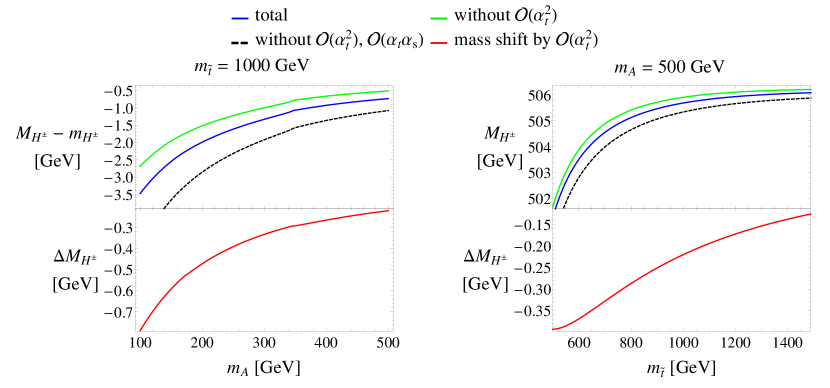
Figure 3: Upper parts: prediction for the charged Higgs-boson mass $M_{H^{\pm}}$ including all known contributions (blue), without the $\mathcal{O}{\left(\alpha_{t}^{2}\right)}$ contributions (green) and without any two-loop corrections (black dashed) [$m_{H^{\pm}}$ is the tree-level mass according to Eq. (6)]. Lower parts: the mass shift $\Delta M_{H^{\pm}}$ by the $\mathcal{O}{\left(\alpha_{t}^{2}\right)}$ contributions (red). Left: $m_{\tilde{t}}\equiv m_{\tilde{q}_{3}}=m_{\tilde{t}_{\text{R}}}=m_{\tilde{b}_{\text{R}}}=1000$ GeV. Right: $m_{A}=500$ GeV. The other input parameters are $t_{\beta}=8$, $\mu=2000$ GeV, $m_{\tilde{\ell}_{3}}=m_{\tilde{\tau}_{\rm R}}=1000$ GeV, $X_{t}=2\,m_{\tilde{t}}$, $A_{b}=A_{\tau}=0$, $m_{\tilde{g}}=1500$ GeV, for both cases.

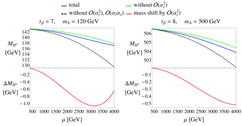
Figure 4: Upper parts: prediction for the charged Higgs-boson mass $M_{H^{\pm}}$ including all known contributions (blue), without the $\mathcal{O}{\left(\alpha_{t}^{2}\right)}$ contributions (green) and without any two-loop corrections (black dashed). Lower parts: the mass shift $\Delta M_{H^{\pm}}$ by the $\mathcal{O}{\left(\alpha_{t}^{2}\right)}$ contributions (red). Left: $t_{\beta}=7$, $m_{A}=120$ GeV, $A_{t}=2.5\,m_{\tilde{q}_{3}}$, $A_{b}=A_{\tau}=0$. Right: $t_{\beta}=8$, $m_{A}=500$ GeV, $X_{t}=2\,m_{\tilde{q}_{3}}$, $A_{b}=A_{\tau}=0$. The other input parameters are $m_{\tilde{q}_{3}}=m_{\tilde{t}_{\text{R}}}=m_{\tilde{b}_{\text{R}}}=1000$ GeV, $m_{\tilde{\ell}_{3}}=m_{\tilde{\tau}_{\rm R}}=1000$ GeV, $m_{\tilde{g}}=1500$ GeV, for both cases.

In all cases, the $\mathcal{O}{\left(\alpha_{t}^{2}\right)}$ contributions appear with negative sign and reduce slightly the positive mass shift arising from $\mathcal{O}{\left(\alpha_{t}\alpha_{s}\right)}$. In general, the combined two-loop corrections result in a positive shift, which can amount to several GeV, on top of the one-loop prediction for $M_{H^{\pm}}$.

In the figures mentioned above, the constraint $m_{h}=125\pm 1\,{\rm GeV}$ on the light Higgs-boson mass is imposed, except for the low-$m_{H}$ scenario in Fig. 4 (left) where it is the heavier $H$-boson that appears with a mass around $125$ GeV (a scenario which may soon be excluded by more stringent limits on the charged Higgs-boson mass). One has to keep in mind, however, that not all of the parameter values in the figures, which are shown for illustrating the parameter dependence, will actually be allowed when more comprehensive phenomenological studies on the properties of the Higgs particle at $125$ GeV will be performed. We have added such a more comprehensive analysis by probing the regions compatible with the experimental constraints by means of the program HiggsBounds Bechtle:2008jh ; Bechtle:2011sb ; Bechtle:2013wla . The result is shown in Fig. 5, where the $\mathcal{O}{\left(\alpha_{t}^{2}\right)}$ effects for $M_{H^{\pm}}$ are displayed for possible combinations of the stop-sector parameters. Also here we find negative mass shifts in the typical range from $-0.5$ GeV to $-0.8$ GeV.

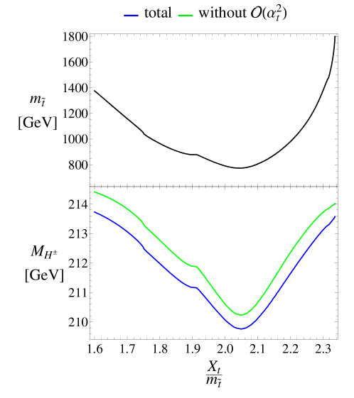
Figure 5: Mass $M_{H^{\pm}}$ of the charged Higgs boson with all available higher-order terms and without the $\mathcal{O}{\left(\alpha_{t}^{2}\right)}$ contributions, for ranges of $m_{\tilde{t}}$ and $X_{t}$ allowed by HiggsBounds and $m_{h}=125$ GeV. Other parameters are $m_{A}=200$ GeV, $t_{\beta}=8$, $\mu=3000$ GeV, $A_{b}=A_{\tau}=0$, $m_{\tilde{\ell}_{3}}=m_{\tilde{\tau}_{\rm R}}=1000$ GeV, $m_{\tilde{g}}=1500$ GeV.

4 Conclusions

We have calculated the two-loop $\mathcal{O}{\left(\alpha_{t}^{2}\right)}$ contributions to the mass $M_{H^{\pm}}$ of the charged Higgs boson when derived from the $A$-boson mass $m_{A}$ as an on-shell input parameter within the real, $CP$-conserving, MSSM and combined them with the complete one-loop and the two-loop $\mathcal{O}{\left(\alpha_{t}^{2}\right)}$ contributions. We have presented numerical studies for scenarios of current phenomenological interest and discussed the effects of the various two-loop terms.

The $\mathcal{O}{\left(\alpha_{t}^{2}\right)}$ two-loop corrections appear with opposite sign and smaller size with respect to the $\mathcal{O}{\left(\alpha_{t}\alpha_{s}\right)}$ contributions; in combination, the two-loop terms yield a positive shift to the mass of the charged Higgs boson as calculated at one-loop order. This shift in $M_{H^{\pm}}$ can be at the level of several GeV and thus of a size that may be relevant for the LHC (and a future electron-positron collider).

The set of two-loop corrections considered here are expected to be particularly relevant in parameter ranges of the real MSSM where the top-Yukawa terms provide a good approximation to the complete one-loop result, especially for relatively low values of $\tan\!\beta$ and $m_{A}$. In this range, besides precise mass predictions, the experimental constraints on the mass and the phenomenological features of the lightest Higgs are important and play a substantial role when comprehensive analyses withing the MSSM Higgs sector are performed.

Our results for the charged Higgs-boson mass have become part of the Fortran code FeynHiggs.

References

- (1) G. Aad et al. [ATLAS Collaboration], Phys. Lett. B 716 (2012) 1 [arXiv:1207.7214 [hep-ex]].
- (2) S. Chatrchyan et al. [CMS Collaboration], Phys. Lett. B 716 (2012) 30 [arXiv:1207.7235 [hep-ex]].
-
(3)
ATLAS Collaboration, see:
https://twiki.cern.ch/twiki/bin/view/AtlasPublic/HiggsPublicResults . -
(4)
CMS Collaboration, see:
https://twiki.cern.ch/twiki/bin/view/CMSPublic/PhysicsResultsHIG . - (5) A. Heister et al. [ALEPH Collaboration], Phys. Lett. B 543 (2002) 1 [arXiv:hep-ex/0207054]; J. Abdallah et al. [DELPHI Collaboration], Eur. Phys. J. C 34 (2004) 399 [arXiv:hep-ex/0404012]; P. Achard et al. [L3 Collaboration], Phys. Lett. B 575 (2003) 208 [arXiv:hep-ex/0309056]; D. Horvath [OPAL Collaboration], Nucl. Phys. A 721 (2003) 453.
- (6) G. Abbiendi et al. [ALEPH and DELPHI and L3 and OPAL and LEP Collaborations], Eur. Phys. J. C 73 (2013) 2463 [arXiv:1301.6065 [hep-ex]].
- (7) T. Aaltonen et al. [CDF Collaboration], Phys. Rev. Lett. 103 (2009) 101803 [arXiv:0907.1269 [hep-ex]]; V. Abazov et al. [DØCollaboration], Phys. Lett. B 682 (2009) 278 [arXiv:0908.1811 [hep-ex]]; P. Gutierrez [CDF and DØCollaborations], PoS CHARGED 2010 (2010) 004.
- (8) G. Aad et al. [ATLAS Collaboration], JHEP 1206 (2012) 039 [arXiv:1204.2760 [hep-ex]]; ATLAS Collaboration, ATLAS-CONF-2013-090; ATLAS-CONF-2014-050; S. Chatrchyan et al. [CMS Collaboration], JHEP 1207 (2012) 143 [arXiv:1205.5736 [hep-ex]]; CMS Collaboration, CMS-HIG-13-035; CMS-HIG-14-020.
- (9) J. A. Casas, J. R. Espinosa, M. Quiros and A. Riotto, Nucl. Phys. B 436 (1995) 3 [Erratum-ibid. B 439 (1995) 466] [hep-ph/9407389]. M. S. Carena, J. R. Espinosa, M. Quiros and C. E. M. Wagner, Phys. Lett. B 355 (1995) 209 [hep-ph/9504316].
-
(10)
S. Heinemeyer, W. Hollik and G. Weiglein,
Phys. Rev. D 58 (1998) 091701
[hep-ph/9803277],
Phys. Lett. B 440 (1998) 296 [hep-ph/9807423]. - (11) S. Heinemeyer, W. Hollik and G. Weiglein, Eur. Phys. J. C 9 (1999) 343 [hep-ph/9812472].
- (12) S. Heinemeyer, W. Hollik and G. Weiglein, Phys. Lett. B 455 (1999) 179 [hep-ph/9903404]. M. S. Carena, H. E. Haber, S. Heinemeyer, W. Hollik, C. E. M. Wagner and G. Weiglein, Nucl. Phys. B 580 (2000) 29 [hep-ph/0001002].
- (13) S. Heinemeyer, W. Hollik, H. Rzehak and G. Weiglein, Eur. Phys. J. C 39 (2005) 465 [hep-ph/0411114].
- (14) S. Borowka, T. Hahn, S. Heinemeyer, G. Heinrich and W. Hollik, Eur. Phys. J. C 74 (2014) 2994 [arXiv:1404.7074 [hep-ph]].
- (15) G. Degrassi, S. Di Vita and P. Slavich, arXiv:1410.3432 [hep-ph].
- (16) R. Harlander, P. Kant, L. Mihaila and M. Steinhauser, Phys. Rev. Lett. 100 (2008) 191602; ibid. 101 (2008) 039901 [arXiv:0803.0672 [hep-ph]], JHEP 1008 (2010) 104 [arXiv:1005.5709 [hep-ph]].
- (17) R.-J. Zhang, Phys. Lett. B 447 (1999) 89 [hep-ph/9808299]. J. R. Espinosa and R.-J. Zhang, Nucl. Phys. B 586 (2000) 3 [hep-ph/0003246], JHEP 0003 (2000) 026 [hep-ph/9912236]. J. R. Espinosa and I. Navarro, Nucl. Phys. B 615 (2001) 82 [hep-ph/0104047]. G. Degrassi, P. Slavich and F. Zwirner, Nucl. Phys. B 611 (2001) 403 [hep-ph/0105096]. R. Hempfling and A. H. Hoang, Phys. Lett. B 331 (1994) 99 [hep-ph/9401219]. A. Brignole, G. Degrassi, P. Slavich and F. Zwirner, Nucl. Phys. B 643 (2002) 79 [hep-ph/0206101]. A. Dedes, G. Degrassi and P. Slavich, Nucl. Phys. B 672 (2003) 144 [hep-ph/0305127].
- (18) J. R. Espinosa and R.-J. Zhang, Nucl. Phys. B 586 (2000) 3 [hep-ph/0003246].
- (19) A. Brignole, G. Degrassi, P. Slavich and F. Zwirner, Nucl. Phys. B 631 (2002) 195 [hep-ph/0112177].
- (20) G. Degrassi, S. Heinemeyer, W. Hollik, P. Slavich and G. Weiglein, Eur. Phys. J. C 28 (2003) 133 [hep-ph/0212020].
- (21) S. Heinemeyer, W. Hollik and G. Weiglein, Phys. Rept. 425, 265 (2006) [hep-ph/0412214].
- (22) B. C. Allanach, A. Djouadi, J. L. Kneur, W. Porod and P. Slavich, JHEP 0409 (2004) 044 [hep-ph/0406166].
- (23) S. P. Martin, Phys. Rev. D 65 (2002) 116003 [hep-ph/0111209], Phys. Rev. D 66 (2002) 096001 [hep-ph/0206136], Phys. Rev. D 67 (2003) 095012 [hep-ph/0211366], Phys. Rev. D 68 (2003) 075002 [hep-ph/0307101], Phys. Rev. D 70 (2004) 016005 [hep-ph/0312092], Phys. Rev. D 71 (2005) 016012 [hep-ph/0405022], Phys. Rev. D 71 (2005) 116004 [hep-ph/0502168]. S. P. Martin and D. G. Robertson, Comput. Phys. Commun. 174 (2006) 133 [hep-ph/0501132].
- (24) D. A. Demir, Phys. Rev. D 60 (1999) 055006 [hep-ph/9901389]. S. Y. Choi, M. Drees and J. S. Lee, Phys. Lett. B 481 (2000) 57 [hep-ph/0002287]. T. Ibrahim and P. Nath, Phys. Rev. D 63 (2001) 035009 [hep-ph/0008237], Phys. Rev. D 66 (2002) 015005 [hep-ph/0204092].
- (25) A. Pilaftsis and C. E. M. Wagner, Nucl. Phys. B 553 (1999) 3 [hep-ph/9902371].
- (26) M. S. Carena, J. R. Ellis, A. Pilaftsis and C. E. M. Wagner, Nucl. Phys. B 586 (2000) 92 [hep-ph/0003180].
- (27) S. Heinemeyer, W. Hollik, H. Rzehak and G. Weiglein, Phys. Lett. B 652 (2007) 300 [arXiv:0705.0746 [hep-ph]].
- (28) M. Frank, T. Hahn, S. Heinemeyer, W. Hollik, H. Rzehak and G. Weiglein, JHEP 0702 (2007) 047 [hep-ph/0611326].
- (29) W. Hollik and S. Paßehr, Phys. Lett. B 733, 144 (2014) [arXiv:1401.8275 [hep-ph]].
- (30) W. Hollik and S. Paßehr, JHEP 1410 (2014) 171 [arXiv:1409.1687 [hep-ph]].
- (31) S. Heinemeyer, W. Hollik and G. Weiglein, Comput. Phys. Commun. 124 (2000) 76 [hep-ph/9812320].
- (32) T. Hahn, S. Heinemeyer, W. Hollik, H. Rzehak and G. Weiglein, Nucl. Phys. Proc. Suppl. 205-206 (2010) 152 [arXiv:1007.0956 [hep-ph]].
- (33) T. Hahn, S. Heinemeyer, W. Hollik, H. Rzehak and G. Weiglein, Comput. Phys. Commun. 180 (2009) 1426.
- (34) J. Gunion and A. Turski, Phys. Rev. D 39 (1989) 2701; Phys. Rev. D 40 (1989) 2333.
-
(35)
A. Brignole, J. Ellis, G. Ridolfi and F. Zwirner,
Phys. Lett. B 271 (1991) 123.
A. Brignole, Phys. Lett. B 277 (1992) 313. -
(36)
M. Diaz and H. Haber,
Phys. Rev. D 45 (1992) 4246;
M. Diaz, PhD thesis: “Radiative Corrections to Higgs Masses in the MSSM”, University of California, Santa Cruz, 1992, SCIPP–92/13. - (37) P. Chankowski, S. Pokorski and J. Rosiek, Phys. Lett. 274 (1992) 191.
- (38) M. Frank, PhD thesis: “Radiative Corrections in the Higgs Sector of the MSSM with Violation”, University of Karlsruhe, 2002, ISBN 3-937231-01-3.
- (39) M. Frank, L. Galeta, T. Hahn, S. Heinemeyer, W. Hollik, H. Rzehak and G. Weiglein, Phys. Rev. D 88 (2013) 055013 [arXiv:1306.1156 [hep-ph]].
- (40) T. Hahn, Comput. Phys. Commun. 140 (2001) 418 [hep-ph/0012260].
- (41) T. Hahn and M. Perez-Victoria, Comput. Phys. Commun. 118 (1999) 153 [hep-ph/9807565].
- (42) G. Weiglein, R. Scharf and M. Böhm, Nucl. Phys. B 416 (1994) 606 [hep-ph/9310358].
- (43) M. Carena, S. Heinemeyer, O. Stål, C. E. M. Wagner and G. Weiglein, Eur. Phys. J. C 73 (2013) 2552 [arXiv:1302.7033 [hep-ph]].
- (44) P. Bechtle, O. Brein, S. Heinemeyer, G. Weiglein and K. E. Williams, Comput. Phys. Commun. 181 (2010) 138 [arXiv:0811.4169 [hep-ph]].
- (45) P. Bechtle, O. Brein, S. Heinemeyer, G. Weiglein and K. E. Williams, Comput. Phys. Commun. 182 (2011) 2605 [arXiv:1102.1898 [hep-ph]].
- (46) P. Bechtle, O. Brein, S. Heinemeyer, O. Stål, T. Stefaniak, G. Weiglein and K. E. Williams, Eur. Phys. J. C 74 (2014) 3, 2693 [arXiv:1311.0055 [hep-ph]].