Multiuser Charging Control in Wireless Power Transfer via Magnetic Resonant Coupling

Abstract

Magnetic resonant coupling (MRC) is a practically appealing method for realizing the near-field wireless power transfer (WPT). The MRC-WPT system with a single pair of transmitter and receiver has been extensively studied in the literature, while there is limited work on the general setup with multiple transmitters and/or receivers. In this paper, we consider a point-to-multipoint MRC-WPT system with one transmitter sending power wirelessly to a set of distributed receivers simultaneously. We derive the power delivered to the load of each receiver in closed-form expression, and reveal a “near-far” fairness issue in multiuser power transmission due to users’ distance-dependent mutual inductances with the transmitter. We also show that by designing the receivers’ load resistances, the near-far issue can be optimally solved. Specifically, we propose a centralized algorithm to jointly optimize the load resistances to minimize the power drawn from the energy source at the transmitter under given power requirements for the loads. We also devise a distributed algorithm for the receivers to adjust their load resistances iteratively, for ease of practical implementation.

I Introduction

Inductive coupling [1, 2, 3] is a conventional method to realize the near-field wireless power transfer (WPT) for short-range applications up to a couple of centimeters. Recently, magnetic resonant coupling (MRC) [5, 6, 7] has drawn significant interests for implementing the near-field WPT due to its high power transfer efficiency for applications requiring longer distances, say, tens of centimeters to several meters. The transmitter and the receiver in an MRC-WPT system are designed to have the same natural frequency as the system’s operating frequency, thereby greatly reducing the total reactive power consumption in the system and achieving high power transfer efficiency over long distances.

The MRC-WPT system with a single pair of transmitter and receiver has been extensively studied in the literature for e.g. maximizing the end-to-end power transfer efficiency or the power delivered to the receiver with a given input power constraint [8, 9, 10, 11]. However, there is limited work on analyzing the MRC-WPT system under the general setup with multiple transmitters and/or receivers. The system with two transmitters and a single receiver or a single transmitter and two receivers has been studied in [12, 13, 14, 15, 16], while their analytical results cannot be applied for a system with more than two transmitters/receivers. Furthermore, to our best knowledge, there has been no work on rigorously establishing a mathematical framework to jointly design parameters in the multi-transmitter/receiver MRC-WPT system for its performance optimization.

In this paper, as shown in Fig. 1, we consider a point-to-multipoint MRC-WPT system, where one transmitter connected to a stable energy source sends wireless power simultaneously to a set of distributed receivers, each of which is connected to a given load. We extend the results in [12, 13, 14, 15, 16] to derive closed-form expressions of the transmit power drawn from the energy source and the power delivered to each load, in terms of various parameters in the system. Our results reveal a near-far fairness issue in the case of multiuser wireless power transmission, similar to its counterpart in wireless communication. Particularly, a receiver that is far away from the transmitter and thus has a small mutual inductance with the transmitter generally receives lower power as compared to a receiver that is close to the transmitter. We then show that the near-far issue can be optimally solved by jointly designing the receivers’ load resistances to control their received power levels, in contrast to the method of adjusting the transmit beamforming weights to control the received power in the far-field microwave transmission based WPT [17, 18].

Specifically, we first study the centralized optimization problem, where a central controller at the transmitter which has the full knowledge of all receivers, including their circuit parameters and load requirements, jointly designs the adjustable load resistances to minimize the total power consumed at the transmitter subject to the given minimum harvested power requirement of each load. Although the formulated problem is non-convex, we develop an efficient algorithm to solve it optimally. Then, for ease of practical implementation, we consider the scenario without any central controller and devise a distributed algorithm for adjusting the load resistances by individual receivers in an iterative manner. In the distributed algorithm, each receiver sets its load resistance independently based on its local information and a one-bit feedback shared by each of the other receivers, where the feedback of each receiver indicates whether the harvested power of its load exceeds the required level or not. Finally, through simulation results, it is shown that the distributed algorithm can achieve close-to-optimal performance as compared to the solution of the centralized optimization.

II System model

We consider an MRC-WPT system with one transmitter and $N$ receivers, indexed by $n$, $n\in{\cal N}=\{1,\ldots,N\}$, as shown in Fig. 1. The transmitter and receivers are equipped with electromagnetic (EM) coils for wireless power transfer. An embedded communication system is also assumed to enable information sharing among the transmitter and/or receivers. The transmitter is connected to a stable energy source supplying sinusoidal voltage over time given by $\tilde{v}_{\text{tx}}(t)=\text{Re}\{{v}_{\text{tx}}e^{jwt}\}$, with ${v}_{\text{tx}}$ denoting a complex voltage which is assumed to be constant, and $w>0$ denoting the operating angular frequency of the system. Each receiver $n$ is also connected to a given load (e.g. a battery charger), named load $n$, with resistance $x_{n}>0$. It is assumed that the transmitter and each receiver $n$ are compensated by series capacitors with capacities $c_{\text{tx}}>0$ and $c_{n}>0$, respectively. Let $\tilde{i}_{\text{tx}}(t)=\text{Re}\{i_{\text{tx}}e^{jwt}\}$, with complex ${i}_{\text{tx}}$, denote the steady state current flowing through the transmitter. This current produces a time-varying magnetic flux in the transmitter’s EM coil, which passes through the receivers’ EM coils and induces time-varying currents in them. We thus denote $\tilde{i}_{n}(t)=\text{Re}\{i_{n}e^{jwt}\}$, with complex ${i}_{n}$, as the steady state current at receiver $n$.

We denote $r_{\text{tx}}>0$ ($r_{n}>0$) and $l_{\text{tx}}>0$ ($l_{n}>0$) as the internal resistance and the self-inductance of the EM coil of the transmitter (receiver $n$), respectively. We also denote the mutual inductance between EM coils of the transmitter and each receiver $n$ by $h_{n}>0$, with $h_{n}\leq\sqrt{l_{n}l_{\text{tx}}}$, where its actual value depends on the physical characteristics of the two EM coils, their locations, alignment or misalignment of their oriented axes with respect to each other, the environment magnetic permeability, etc. For example, the mutual inductance of two coaxial circular loops that lie in the parallel planes with separating distance of $d$ meter is approximately proportional to $d^{-3}$ [4]. Moreover, since the receivers usually employ smaller EM coils than that of the transmitter due to size limitations and they are also physically separated, we can safely ignore the mutual inductance between any pair of them. The equivalent electric circuit model of the considered MRC-WPT system is shown in Fig. 1,

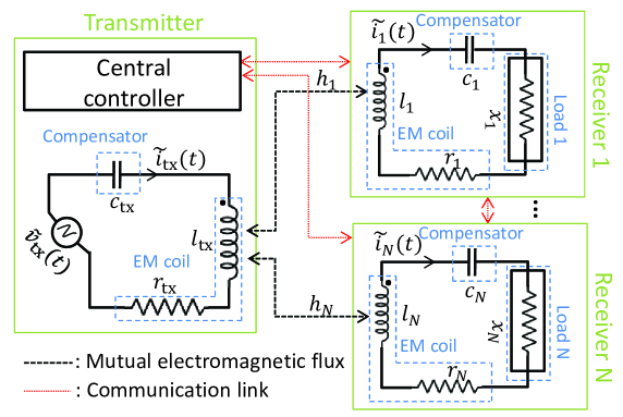
Figure 1: A point-to-multipoint MRC-WPT system with communication and control.

in which the natural angular frequencies of the transmitter and each receiver $n$ are given by $w_{\text{tx}}={1}/{\sqrt{l_{\text{tx}}c_{\text{tx}}}}$ and $w_{n}={1}/{\sqrt{l_{n}c_{n}}}$, respectively. We set $c_{\text{tx}}=l_{\text{tx}}^{-1}w^{-2}$ and $c_{n}=l_{n}^{-1}w^{-2}$, $\forall n\in\cal N$, to ensure that the transmitter and all receivers have the same natural frequency as the system’s operating frequency $w$, named resonant angular frequency, i.e., $w_{\text{tx}}=w_{1}=\ldots=w_{N}=w$.

We assume that the transmitter and all receivers are at fixed positions and the physical characteristics of their EM coils are known; thus, $h_{n}$, $\forall n\in\cal N$, are modeled as given constants. We treat the receivers’ load resistances $x_{n}$, $\forall n\in\cal N$, as design parameters, which can be adjusted in real-time [15] to control the performance of the MRC-WPT system based on the information shared among different nodes in the system via wireless communication.

III Performance Analysis

In this section, we first present our analytical results. A numerical example is then provided to draw useful insights from the analysis.

III-A Analytical Results

Define $\mbox{\boldmath{$v$}}=[v_{\text{tx}},{\bf 0}_{1\times N}]^{T}$ and $\mbox{\boldmath{$i$}}=[i_{\text{tx}},{i}_{1},\ldots,{i}_{N}]$, where $v$ is the voltage vector and $i$ is the current vector that can be obtained as a function of $v$. Let $\mbox{\boldmath{$R$}}=\text{Diag}(r_{1},\ldots,r_{N})$, $\mbox{\boldmath{$X$}}=\text{Diag}(x_{1},\ldots,x_{N})$, and $\mbox{\boldmath{$h$}}=[h_{1},\ldots,h_{N}]^{T}$. By applying Kirchhoff’s circuit laws to the electric circuit model in Fig. 1, we obtain

$$\mbox{\boldmath{$i$}}=\left[\begin{array}[]{cc}r_{\text{tx}}&-jw\mbox{\boldmath{$h$}}^{T}\\ -jw\mbox{\boldmath{$h$}}&\mbox{\boldmath{$R$}}+\mbox{\boldmath{$X$}}\end{array}\right]^{-1}\mbox{\boldmath{$v$}}=\mbox{\boldmath{$A$}}^{-1}\mbox{\boldmath{$v$}},$$ (3)

where $\mbox{\boldmath{$A$}}\in\mathbb{C}^{(N+1)\times(N+1)}$ is called the impedance matrix. The determinant of $A$ is given by

$$\text{det}(\mbox{\boldmath{$A$}})=\big{(}r_{\text{tx}}+w^{2}\sum_{k=1}^{N}h_{k}^{2}(r_{k}+x_{k})^{-1}\big{)}\big{(}\prod_{k=1}^{N}r_{k}+x_{k}\big{)},$$ (4)

where it can be easily verified that $\text{det}(\mbox{\boldmath{$A$}})>0$. Then, we define $\mbox{\boldmath{$B$}}=\mbox{\boldmath{$A$}}^{-1}$, which is called the admittance matrix. Let $\mbox{\boldmath{$B$}}(b,l)$ denote the element in row $b$ and column $l$ of $B$. We simplify (3) as

$$\mbox{\boldmath{$i$}}=\left[\mbox{\boldmath{$B$}}(1,1),\ldots,\mbox{\boldmath{$B$}}(N+1,1)\right]^{T}v_{\text{tx}}.$$ (5)

It can also be shown that $\mbox{\boldmath{$B$}}(b,1)$, $b\in\{1,\ldots,N+1\}$, is given by

$$\mbox{\boldmath{$B$}}(b,1)=\left\{\begin{array}[]{rl}~{}\dfrac{1}{r_{\text{tx}}+w^{2}\sum_{k=1}^{N}h_{k}^{2}(r_{k}+x_{k})^{-1}}&\text{if}~{}~{}b=1,\\ j\dfrac{wh_{b-1}(r_{b-1}+x_{b-1})^{-1}}{r_{\text{tx}}+w^{2}\sum_{k=1}^{N}h_{k}^{2}(r_{k}+x_{k})^{-1}}&\text{otherwise}.\end{array}\right.$$ (6)

By substituting (6) into (5), it follows that

$$i_{\text{tx}} =~{}\dfrac{1}{r_{\text{tx}}+w^{2}\sum_{k=1}^{N}h_{k}^{2}(r_{k}+x_{k})^{-1}}v_{\text{tx}},$$ (7)

$$i_{n} =j\dfrac{wh_{n}(r_{n}+x_{n})^{-1}}{r_{\text{tx}}+w^{2}\sum_{k=1}^{N}h_{k}^{2}(r_{k}+x_{k})^{-1}}v_{\text{tx}},~{}\forall n\in\cal N.$$ (8)

The power drawn from the energy source, denoted by $p_{\text{tx}}$, and that delivered to each load $n$, denoted by $p_{n}$, are then obtained as

$$p_{\text{tx}} =\dfrac{1}{2}\text{Re}\{v_{\text{tx}}i_{\text{tx}}^{*}\}=\dfrac{|v_{\text{tx}}|^{2}}{2}\dfrac{1}{\hskip 9.3894ptr_{\text{tx}}+w^{2}\sum_{k=1}^{N}h_{k}^{2}(r_{k}+x_{k})^{-1}\hskip 2.84526pt},$$ (9)

$$p_{n} =\hskip 3.27205pt\dfrac{1}{2}x_{n}|i_{n}|^{2}\hskip 3.27205pt=\dfrac{|v_{\text{tx}}|^{2}}{2}\dfrac{w^{2}h_{n}^{2}x_{n}(r_{n}+x_{n})^{-2}}{(r_{\text{tx}}+w^{2}\sum_{k=1}^{N}h_{k}^{2}(r_{k}+x_{k})^{-1})^{2}},$$ (10)

where $i_{\text{tx}}^{*}$ is the conjugate of $i_{\text{tx}}$. From (10), it follows that the power delivered to each load $n$ increases with the mutual inductance between EM coils of its receiver and the transmitter, i.e., $h_{n}$. This can potentially cause a near-far fairness issue since a receiver that is far away from the transmitter in general has a small mutual inductance with the transmitter; thus, its received power is lower than a receiver that is close to the transmitter (with a larger mutual inductance). We accordingly define $p_{\text{sum}}=\sum_{n=1}^{N}p_{n}$ as the sum (aggregate) power delivered to all loads, where we always have $p_{\text{sum}}<p_{\text{tx}}$.

In the following, we study impacts of changing the load resistance of one particular receiver $n$, i.e., $x_{n}$, on the transmitter power $p_{\text{tx}}$, its received power $p_{n}$ and that delivered to each of the other loads $m\in\cal N$, $m\neq n$, i.e., $p_{m}$, as well as the sum power delivered to all loads $p_{\text{sum}}$, assuming that all other load resistances are fixed.

Property 1.

$p_{\textnormal{tx}}$ strictly increases over $x_{n}>0$.

This result can be explained as follows. From (7), it is observed that the transmitter current $i_{\text{tx}}$ strictly increases over $x_{n}>0$. Hence, due to the fact that the energy source voltage $v_{\text{tx}}$ is fixed, it follows that $p_{\text{tx}}$ given in (9) strictly increases over $x_{n}>0$.

Property 2.

$p_{m}$, $\forall m\neq n$, strictly increases over $x_{n}>0$. However, $p_{n}$ first increases over $0<x_{n}<\dot{x}_{n}$, and then decreases over $x_{n}>\dot{x}_{n}$, where

$$\dot{x}_{n}=\big{(}{r_{n}(r_{\textnormal{tx}}+\phi_{n})+w^{2}h_{n}^{2}}\big{)}/\big{(}{r_{\textnormal{tx}}+\phi_{n}}\big{)},$$ (11)

with $\phi_{n}=w^{2}\sum_{k\neq n}h_{k}^{2}(r_{k}+x_{k})^{-1}$.

The above result can be justified as follows. From (8), it follows that for each receiver $m$, $m\neq n$, its current $i_{m}$ strictly increases over $x_{n}>0$. This is because $i_{\text{tx}}$ increases with $x_{n}$, and as a result, $i_{m}$ increases due to the mutual coupling between EM coils of receiver $m$ and the transmitter. Hence, the received power $p_{m}$ defined in (10) also strictly increases over $x_{n}>0$. On the other hand, it follows from (8) that for receiver $n$, its current $i_{n}$ strictly decreases over $x_{n}>0$. Moreover, from (10), it follows that the decrement in $|i_{n}|^{2}$ is smaller than the increment of $x_{n}$ when $0<x_{n}<\dot{x}_{n}$; thus, $p_{n}$ increases with $x_{n}$ in this region, while the opposite is true when $x_{n}>\dot{x}_{n}$.

Property 3.

If $r_{\textnormal{tx}}+\phi_{n}-2\varphi_{n}\leq 0$, $p_{\textnormal{sum}}$ strictly increases over $x_{n}>0$, where $\varphi_{n}=w^{2}\sum_{k\neq n}h_{k}^{2}x_{k}(r_{k}+x_{k})^{-2}$; otherwise, $p_{\textnormal{sum}}$ first increases over $0<x_{n}<\ddot{x}_{n}$, and then decreases over $x_{n}>\ddot{x}_{n}$, where

$$\ddot{x}_{n}=\big{(}{r_{n}(r_{\textnormal{tx}}+\phi_{n})+w^{2}h_{n}^{2}+2r_{n}\varphi_{n}}\big{)}/\big{(}{r_{\textnormal{tx}}+\phi_{n}-2\varphi_{n}}\big{)}.$$ (12)

This property is a direct consequence of Property 2.

III-B Numerical Example

We consider an MRC-WPT system with $N=3$ receivers, where $v_{\text{tx}}=25\sqrt{2}$V, $r_{\text{tx}}=0.35\Omega$, $l_{\text{tx}}=6.35\mu$H, $r_{n}=0.15\Omega$, $l_{n}=0.85\mu$H, $\forall n\in\cal N$, $\mbox{\boldmath{$h$}}=[2.3,1.1,0.9]\mu$H, and $w=2.2\times 10^{6}$rad/s. In this example, receiver $1$ is closest to the transmitter and thus it has the largest mutual inductance, while receiver $3$ is farthest. For the purpose of exposition, we fix $x_{2}=x_{3}=7.5\Omega$. We plot $p_{\text{tx}}$, $p_{n}$, $\forall n\in\cal N$, and $p_{\text{sum}}$, versus the resistance of load $1$, $x_{1}$, in Fig. 2.

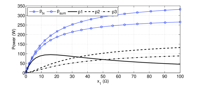
Figure 2: Input and output power versus $x_{1}$.

It is observed that $p_{\text{tx}}$, $p_{2}$, $p_{3}$ and $p_{\text{sum}}$ all increase over $x_{1}>0$. Note that in this example, the condition $r_{\textnormal{tx}}+\phi_{n}-2\varphi_{n}\leq 0$ holds in Property 3. However, $p_{1}$ first increases over $0<x_{1}<\dot{x}_{1}=15.8\Omega$, and then declines over $x_{1}>15.8\Omega$. These results are consistent with our above analysis. Finally, we point out that changing $x_{1}$ not only affects $p_{1}$, but also the power delivered to other loads. For instance, receiver $1$ can help receivers $2$ and $3$, which are farther away from the transmitter, to receive higher power by increasing $x_{1}$. This is a useful mechanism that will be utilized to solve the near-far issue.

IV Centralized Optimization

In this section, we optimize the receivers’ load resistances $x_{n}$, $\forall n\in\cal N$, to minimize the power drawn from the energy source at the transmitter subject to the given load constraints. We assume a central controller at the transmitter, which has full knowledge of the receivers, including their circuit parameters and load requirements, to implement the proposed centralized optimization.

IV-A Problem Formulation

We assume that the resistance of each load $n$ can be adjusted over a given range $\underline{x}_{n}\leq x_{n}\leq\overline{x}_{n}$, where $\underline{x}_{n}>0$ and $\overline{x}_{n}\geq\underline{x}_{n}$ are lower and upper limits of $x_{n}$ due to practical considerations. We also assume that the power delivered to each load $n$ should be higher than a certain power threshold $\underline{p}_{n}>0$. Hence, we formulate the following optimization problem to minimize the power drawn from the energy source at the transmitter.

$$\mathrm{(P1)}: \mathop{\mathtt{min}}_{\{\underline{x}_{n}\leq x_{n}\leq\overline{x}_{n}\}}~{}\dfrac{|v_{\text{tx}}|^{2}}{2}\dfrac{1}{r_{\text{tx}}+w^{2}\sum_{k=1}^{N}h_{k}^{2}(r_{k}+x_{k})^{-1}}$$

$$\mathtt{s.t.} ~{}\dfrac{|v_{\text{tx}}|^{2}}{2}\dfrac{w^{2}h_{n}^{2}x_{n}(r_{n}+x_{n})^{-2}}{(r_{\text{tx}}+w^{2}\sum_{k=1}^{N}h_{k}^{2}(r_{k}+x_{k})^{-1})^{2}}\geq\underline{p}_{n},~{}\forall n\in\cal N.$$

(P1) is a non-convex optimization problem. However, in the next we propose an efficient algorithm to solve (P1) optimally.

IV-B Proposed Algorithm

We define an auxiliary variable $z=1/(r_{\text{tx}}+w^{2}\sum_{k=1}^{N}h_{k}^{2}(r_{k}+x_{k})^{-1})\geq 0$. Since $\underline{x}_{n}\leq x_{n}\leq\overline{x}_{n}$, $\forall n\in\cal N$, we have $\underline{z}\leq z\leq\overline{z}$, where $\underline{z}=1/(r_{\text{tx}}+w^{2}\sum_{k=1}^{N}h_{k}^{2}(r_{k}+\underline{x}_{k})^{-1})$ and $\overline{z}=1/(r_{\text{tx}}+w^{2}\sum_{k=1}^{N}h_{k}^{2}(r_{k}+\overline{x}_{k})^{-1})$. Then, we rewrite (P1) as

$$\mathrm{(P2)}:\hskip 14.22636pt \mathop{\mathtt{min}}_{\{\underline{x}_{n}\leq x_{n}\leq\overline{x}_{n}\},~{}\underline{z}\leq z\leq\overline{z}}~{}{|v_{\text{tx}}|^{2}}~{}z/{2}$$

$$\mathtt{s.t.} ~{}\dfrac{|v_{\text{tx}}|^{2}}{2}z^{2}w^{2}h_{n}^{2}x_{n}(r_{n}+x_{n})^{-2}\geq\underline{p}_{n},~{}\forall n\in\cal N$$ (13)

$$~{}r_{\text{tx}}+w^{2}\sum_{k=1}^{N}h_{k}^{2}(r_{k}+x_{k})^{-1}=z^{-1}.$$ (14)

Although (P2) is still non-convex, we can solve it in an iterative manner by searching for the smallest $z$, $\underline{z}\leq z\leq\overline{z}$, under which (P2) is feasible. Staring from $z=\underline{z}$, we test the feasibility of (P2) given $z$ by considering the following problem.

$$\mathrm{(P3)}:\mathop{\mathtt{Find}} ~{}\{\underline{x}_{n}\leq x_{n}\leq\overline{x}_{n},~{}\mathtt{s.t.}(\ref{problem8:const1})\text{ and }(\ref{problem8:const2})\}.$$

If (P3) is feasible, then we set the optimal objective value of (P2) as $z$, which can be attained by any feasible solutions to (P3). Otherwise, we set $z=z+\Delta z$, where $\Delta z>0$ is a small step size. We repeat the above procedure until (P3) becomes feasible or $z>\overline{z}$. The following proposition summarizes the feasibility conditions for (P3).

Proposition 1.

Given $z$, with $\underline{z}\leq z\leq\overline{z}$, (P3) is feasible if and only if all conditions listed below hold at the same time:

• $z\geq 2\sqrt{r_{n}/\alpha_{n}}$, $\forall n\in\cal N$, where $\alpha_{n}=|v_{\text{tx}}|^{2}w^{2}h_{n}^{2}/(2\underline{p}_{n})$.

• ${x}_{n}^{\text{L}}\leq\underline{x}_{n}\leq{x}_{n}^{\text{U}}$ and/or ${x}_{n}^{\text{L}}\leq\overline{x}_{n}\leq{x}_{n}^{\text{U}}$, $\forall n\in\cal N$, where ${x}_{n}^{L}=(\alpha_{n}z^{2}/2-r_{n})-z\sqrt{\alpha_{n}(\alpha_{n}z^{2}/4-r_{n})}$ and ${x}_{n}^{U}=(\alpha_{n}z^{2}/2-r_{n})+z\sqrt{\alpha_{n}(\alpha_{n}z^{2}/4-r_{n})}$.

• $\Phi=\{(y_{1},\ldots,y_{N})~{}|~{}\underline{y}_{n}\leq y_{n}\leq\overline{y}_{n},~{}\forall n\in{\cal N},~{}r_{\text{tx}}+w^{2}\sum_{k=1}^{k=N}h_{k}^{2}y_{k}=z^{-1}\}\neq\emptyset$, where $\underline{y}_{n}=1/(r_{n}+\min\{\overline{x},~{}{x}_{n}^{U}\})$, and $\overline{y}_{n}=1/(r_{n}+\max\{\underline{x},~{}{x}_{n}^{L}\})$.

Given any $(y_{1},\ldots,y_{n})\in\Phi$, where $\Phi$ is given in C3 of Proposition 1, the corresponding feasible solution to (P3) is obtained by a change of variable as $x_{n}=1/y_{n}-r_{n}$, $\forall n\in\cal N$. Note that the obtained $(x_{1},\ldots,x_{N})$ solves (P1) optimally. To summarize, the algorithm to solve (P1) is given in Table 1, denoted by Algorithm 1.

TABLE I: Algorithm for optimally solving (P1).

 Algorithm 1  

• Given $\underline{x}_{n}>0$ and $\overline{x}_{n}>\underline{x}_{n}$, $\forall n\in\cal N$, compute $\underline{z}$ and $\overline{z}$. Initialize $z\leftarrow\underline{z}$, $\Delta z>0$, and $Flag\leftarrow 0$.

• While $z<\overline{z}$ and $Flag=0$ do:

  • Given $z$, check the conditions listed in Proposition 1.

  • If at least one condition does not hold, then set $z=z+\Delta z$. Otherwise, set $Flag=1$. Choose any $(y_{1},\ldots,y_{n})\in\Phi$, where the set $\Phi$ is given in condition C3 of Proposition 1. Set $x_{n}=1/y_{n}-r_{n}$, $\forall n\in\cal N$.

• If $Flag=1$, then return $(x_{1},\ldots,x_{N})$ as the optimal solution to (P1). Otherwise, problem (P1) is infeasible.

 

V Distributed Algorithm

In this section, we present a distributed algorithm for (P1), where it is suitable for practical implementation when a central controller is not available in the system. In this algorithm, each receiver adjusts its load resistance independently according to its local information and a one-bit feedback from each of the other receivers indicating whether the corresponding load constraint is satisfied or not. We denote the feedback from each receiver $n$ which is broadcast to all other receivers as $FB_{n}\in\{0,1\}$, where $FB_{n}=1$ ($FB_{n}=0$) indicates that its load constraint is (not) satisfied.

In Section III, we show that the power delivered to each load $n$, i.e., $p_{n}$, has two properties that can be exploited to adjust $x_{n}$. First, $p_{n}$ strictly increases over $x_{m}>0$, $\forall m\neq n$, which means that other receivers can help boost $p_{n}$ by increasing their load resistances. Second, $p_{n}$ has a single peak at $x_{n}=\dot{x}_{n}$, assuming that other load resistances are all fixed. Thus, over $0<x_{n}<\dot{x}_{n}$, receiver $n$ can increase $p_{n}$ by increasing $x_{n}$; similarly, for $x_{n}>\dot{x}_{n}$, it can increase $p_{n}$ by reducing $x_{n}$. Although receiver $n$ cannot compute $\dot{x}_{n}$ from (11) directly due to its incomplete information on other receivers, it can test whether $0<x_{n}<\dot{x}_{n}$, $x_{n}=\dot{x}_{n}$, or $x_{n}>\dot{x}_{n}$ as follows. Let $p_{n}({x_{n}^{+}})$, $p_{n}({x_{n}})$, and $p_{n}(x_{n}^{-})$ be the power received by load $n$ when its resistance is set as $x_{n}+\Delta x$, $x_{n}$, and $x_{n}-\Delta x$, respectively, where $\Delta x>0$ is a small step size. Assuming all the other load resistances are fixed, receiver $n$ can make the following decision:
$\bullet$ If $p_{n}({x_{n}^{+}})>p_{n}({x_{n}})$ and $p_{n}({x_{n}^{-}})<p_{n}({x_{n}})$, then $0<x_{n}<\dot{x}_{n}$;
$\bullet$ If $p_{n}({x_{n}^{+}})<p_{n}({x_{n}})$ and $p_{n}({x_{n}^{-}})<p_{n}({x_{n}})$, then $x_{n}=\dot{x}_{n}$;
$\bullet$ If $p_{n}({x_{n}^{+}})<p_{n}({x_{n}})$ and $p_{n}({x_{n}^{-}})>p_{n}({x_{n}})$, then $x_{n}>\dot{x}_{n}$.

Next, we present the distributed algorithm in detail. The algorithm is implemented in an iterative manner, say, starting from receiver 1, where in each iteration, only one receiver $n$ adjusts its load resistance, while all the other receivers just broadcast their individual one-bit feedback $FB_{m}$, $m\neq n$, at the beginning of each iteration. Initialize by randomized $x_{n}\in[\underline{x}_{n},~{}\overline{x}_{n}]$, $\forall n\in\cal N$. At each iteration for receiver $n$, if $p_{n}<\underline{p}_{n}$, then it will adjust $x_{n}$ to increase $p_{n}$. To find the correct direction for the update, it needs to check for its current $x_{n}$ whether $0<x_{n}<\dot{x}_{n}$, $x_{n}=\dot{x}_{n}$, or $x_{n}>\dot{x}_{n}$ holds, using the method mentioned in the above. On the other hand, if $p_{n}>\underline{p}_{n}$, receiver $n$ can increase $x_{n}$ to help increase the power delivered to other loads when there exists any $m\neq n$ such that $FB_{m}=0$ is received; or it can decrease $x_{n}$ to help reduce the transmitter power when $FB_{m}=1$, $\forall m\neq n$. In summary, we design the following protocol (with five cases) for receiver $n$ to update $x_{n}$.
C1:  If  $p_{n}\hskip 1.5649pt<\hskip 1.42262pt\underline{p}_{n}$ and $0<x_{n}<\dot{x}_{n}$, set $x_{n}\leftarrow\min\{\overline{x}_{n},x_{n}+\Delta x\}$.
C2:  If  $p_{n}\hskip 1.5649pt<\hskip 1.42262pt\underline{p}_{n}$ and $x_{n}>\dot{x}_{n}$, set $x_{n}\leftarrow\max\{\underline{x}_{n},x_{n}-\Delta x\}$.
C3: If $p_{n}>\underline{p}_{n}$, $x_{n}\neq\dot{x}_{n}$, and $\exists m\neq n$, $FB_{m}=0$, set $x_{n}\leftarrow\min\{\overline{x}_{n},x_{n}+\Delta x\}$.
C4: If $p_{n}>\underline{p}_{n}$, $x_{n}\neq\dot{x}_{n}$, and $FB_{m}=1$, $\forall m\neq n$, set $x_{n}\leftarrow\max\{\underline{x}_{n},x_{n}-\Delta x\}$.
C5: Otherwise, no update occurs.

In addition, we assume that there is a maximum number of iterations, denoted by $K_{\max}>1$, after which the algorithm will terminate, regardless of whether it converges to a stable point $(x_{1},\ldots,x_{N})$ or not. However, when the algorithm converges/terminates, the power constraints given in (13) may or may not hold for all loads, depending on the initial values of $x_{n}$’s. If constraint (13) holds for all loads, then the obtained $(x_{1},\ldots,x_{N})$ is a suboptimal solution to (P1); otherwise, it is infeasible for (P1). The distributed algorithm is summarized in Table 2, as Algorithm 2.

TABLE II: Distributed algorithm for (P1).

 Algorithm 2  

• Initialize $Itr=1$ and $K_{\max}\geq 1$. Each receiver $n$ randomly chooses $x_{n}\in[\underline{x}_{n},~{}\overline{x}_{n}]$.

• Repeat from receiver $n=1$ to $n=N$:

  • Receiver $n$ receives $FB_{m}$ from all other receivers $m\neq n$ and updates its load resistance $x_{n}$ according cases C1–C5.

  • If   $Itr=K_{\max}$, then quit the loop and the algorithm terminates.

  • Set $Itr=Itr+1$.

 

VI Simulation Results

We consider the same system setup as that in Section III-B. We set $\underline{x}_{n}=0.01\Omega$ and $\overline{x}_{n}=100\Omega$, $\forall n\in\cal N$. We also set $\underline{p}_{1}=250$W, $\underline{p}_{2}=50$W, and $\underline{p}_{3}$ varying as $0<\underline{p}_{3}\leq 50$W. Note that (P1) is feasible under the above setting. For Algorithm 1, we use $\Delta z=10^{-3}$. For Algorithm 2, we use $\Delta x=10^{-3}$ and $K_{\max}=10^{5}$, which is sufficiently large such that the algorithm converges to a stable point, while there is no guarantee that the power constraints given in (13) hold for all loads at this point. Therefore, to evaluate the performance of Algorithm 2, we averaged its result over 200 randomly generated initial points for each of which the algorithm converged to a feasible solution to (P1). In Fig. 3, we plot $p_{\text{tx}}$ versus $p_{3}$.

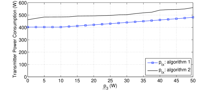
Figure 3: Performance comparison of Algorithms 1 and 2.

It is observed that $p_{\text{tx}}$ obtained by Algorithm $1$ is lower than that by Algorithm $2$, while the gap is quite small, for all values of $\underline{p}_{3}$. This is expected since Algorithm $1$ solves (P1) optimally, while Algorithm 2 in general only returns a suboptimal solution.

VII Conclusion

In this paper, we study a point-to-multipoint MRC-WPT system with distributed receivers. We derive closed-form expressions for the input and output power in terms of the system parameters. Similar to other multiuser wireless applications such as those in wireless communication and far-field microwave based WPT, a near-far fairness issue is revealed in our considered system. To tackle this problem, we propose a centralized algorithm for jointly optimizing the receivers’ load resistances to minimize the transmitter power subject to the given load constraints. For ease of practical implementation, we also devise a distributed algorithm for receivers to iteratively adjust their load resistances based on local information and one-bit feedback from each of the other receivers. We show by simulation that the distributed algorithm performs sufficiently close to the centralized algorithm with a finite number of iterations. As a concluding remark, MRC-WPT is a promising research area for which many tools from signal processing and optimization can be applied to devise new solutions, and we hope that this paper will open up an avenue for future work along this direction.

References

- [1] J. Murakami, F. Sato, T. Watanabe, H. Matsuki, S. Kikuchi, K. Harakawa, and T. Satoh, “Consideration on cordless power station-contactless power transmission system,” IEEE Trans. Magn., vol. 32, no. 5, pp. 5037-5039, Sep. 1996.
- [2] Y. T. Jang and M. M. Jovanovic, “A contactless electrical energy transmission system for portable-telephone battery chargers,” IEEE Trans. Ind. Electron., vol. 50, no. 3, pp. 520-527, June 2003.
- [3] V. J. Brusamarello, Y. B. Blauth, R. Azambuja, I. Muller, and F. Sousa, “Power transfer with an inductive link and wireless tuning,” IEEE Trans. Instrum. Meas., vol. 62, no. 5, pp. 924-931, May 2013.
- [4] D. Cheng, Field and wave electromagnetics, Addison Wesley, 1983.
- [5] A. Kurs, A. Karalis, R. Moffatt, J. D. Joannopoulos, P. Fisher, and M. Soljacic, “Wireless power transfer via strongly coupled magnetic resonances,” Science, vol. 317, no. 83, pp. 83-86, July 2007.
- [6] J. Shin, S. Shin, Y. Kim, S. Ahn, S. Lee, G. Jung, S. Jeon, and D. Cho, “Design and implementation of shaped magnetic-resonance-based wireless power transfer system for roadway-powered moving electric vehicles,” IEEE Trans. Ind. Electron., vol. 61, no. 3, pp. 1179-1192, Mar. 2014.
- [7] L. Chen, Y. C. Zhou, and T. J. Cui, “An optimizable circuit structure for high-efficiency wireless power transfer,” IEEE Trans. Ind. Electron., vol. 60, no. 1, pp. 339-349, Jan. 2013.
- [8] B. L. Cannon, J. F. Hoburg, D. Stancil, and S. Goldstein, “Magnetic resonant coupling as a potential means for wireless power transfer to multiple small receivers,” IEEE Trans. Power Electron., vol. 24, no. 7, pp. 1819-1825, July 2009.
- [9] O. Jonah, S. Georgkopoulos, and M. Tentzeris, “Optimal design parameters for wireless power transfer by resonance magnetic,” IEEE Antennas Wireless Propagat. Lett., vol. 11, pp. 1390-1393, Nov. 2012.
- [10] Y. Zhang and Z. Zhao, “Frequency splitting analysis of two-coil resonant wireless power transfer,” IEEE Antennas Wireless Propagat. Lett., vol. 13, pp. 400-402, Feb. 2014.
- [11] Y. Zhang, Z. Zhao, and K. Chen, “Frequency decrease analysis of resonant wireless power transfer,” IEEE Trans. Power Electron., vol. 29, no. 13, pp. 1058-1063, Mar. 2014.
- [12] I. Yoon and H. Ling, “Investigation of near-field wireless power transfer under multiple transmitters,” IEEE Antennas Wireless Propagat. Lett., vol. 10, pp. 662-665, June 2011.
- [13] K. Lee and D. Cho, “Diversity analysis of multiple transmitters in wireless power transfer system,” IEEE Trans. Magnetics, vol. 49, no. 6, pp. 2946-2952, June 2013.
- [14] D. Ahn and S. Hong, “Effect of coupling between multiple transmitters or multiple receivers on wireless power transfer,” IEEE Trans. Ind. Electron., vol. 60, no. 7, pp. 2602-2613, July 2013.
- [15] J. Garnica, R. Chinga, and J. Lin, “Wireless power transmission: from far field to near field,” Proceedings of the IEEE, vol. 101, no. 6, pp. 1321-1331, June 2013.
- [16] R. Johari, J. Krogmeier, and D. Love, “Analysis and practical considerations in implementing multiple transmitters for wireless power transfer via coupled magnetic resonance,” IEEE Trans. Ind. Electron., vol. 61, no. 4, pp. 1174-1783, Apr. 2014.
- [17] R. Zhang and C. K. Ho, “MIMO broadcasting for simultaneous wireless information and power transfer,” IEEE Trans. Wireless Commun., vol. 12, no. 5, pp. 1989-2001, May 2013.
- [18] J. Xu and R. Zhang, “Energy beamforming with one-bit feedback,” IEEE Trans. Signal Process., vol. 62, no. 20, pp. 5370-5381, Oct. 2014.
- [19] S. Boyd and L. Vandenberghe, Convex optimization, Cambridge University Press, 2004.