Sparse Coding with Earth Mover’s Distance for Multi-Instance Histogram Representation

Abstract

Sparse coding (Sc) has been studied very well as a powerful data representation method. It attempts to represent the feature vector of a data sample by reconstructing it as the sparse linear combination of some basic elements, and a $L_{2}$ norm distance function is usually used as the loss function for the reconstruction error. In this paper, we investigate using Sc as the representation method within multi-instance learning framework, where a sample is given as a bag of instances, and further represented as a histogram of the quantized instances. We argue that for the data type of histogram, using $L_{2}$ norm distance is not suitable, and propose to use the earth mover’s distance (EMD) instead of $L_{2}$ norm distance as a measure of the reconstruction error. By minimizing the EMD between the histogram of a sample and the its reconstruction from some basic histograms, a novel sparse coding method is developed, which is refereed as SC-EMD. We evaluate its performances as a histogram representation method in tow multi-instance learning problems — abnormal image detection in wireless capsule endoscopy videos, and protein binding site retrieval. The encouraging results demonstrate the advantages of the new method over the traditional method using $L_{2}$ norm distance.

1 Introduction

Sparse Coding (SC) has been recently proposed and studied well as an effective data representation method in machine learning community Lee2007 ; Yang20091794 ; Mairal201019 ; Yang201545 ; Bai2015 ; Representing2015 . Given a set of basic elements and a data sample, SC tries to represent the sample by reconstructing it as a linear combination of these basic elements. The linear combination coefficient vector could be used as the new representation of the sample. To this end, the basic elements and the coefficient vector (also called coding vector) are learned by minimizing the reconstruction error. At the same time, we also hope that the coding vector could be as sparse as possible. To measure the reconstruction error, a squared $L_{2}$ norm distance is usually applied to compare the original feature vector and its sparse linear combination as a loss function. At the same time, a $L_{1}$ norm regularization term is also imposed to the coding vector to seek its sparsity. The advantage of using the $L_{2}$ norm distance to as the loss function and using $L_{1}$ norm regularization for sparsity purpose lies on that it is easy to optimize and interpret. The feature-sign search method had been proposed to solve the SC problem by Lee et al. in Lee2007 . Some different SC versions had also be proposed since then, by adding different bias terms to the original SC loss function based on $L_{2}$ norm distance LapSC2010 ; GraphSC2011 ; Gao2013 .

In the multi-instance learning framework, each sample is given as a bag of multiple instances, instead of one single instance in the traditional machine learning problem Zhou20091249 ; Zhou2005135 ; Zhou20071609 ; Du201551 . For example, in image classification and retrieval problems, an image could be split into many small image patches, and each patch is an instance. In this case, we usually first learn a set of instance prototypes by clustering the instances of the training samples, and then represent a sample by quantizing its instances into the instance prototypes, and obtain a quantization histogram Tsai2009100 ; Lu2005956 ; Kotani2002II105 . The normalized histogram is used as the feature vector of the sample for further classification or retrieval task. When we try to apply the SC to represent the histogram data samples under the multi-instance learning framework, directly using $L_{2}$ norm distance may not be suitable anymore. Other distance functions which is especially suitable for histogram data is desired. In fact, many distance functions have been studied for histogram data comparison, such as Kullback — Leibler divergence Seghouane200797 ; Rached2004917 ; Hershey2007IV317 , $\chi^{2}$ distance Huong20091310 ; Emran200219 ; Ye2006393 , Earth Mover’s Distance (EMD) Levina2001251 ; Ling2007840 ; Rubner200099 , etc. Among these distance functions, the EMD metric has been known to quantify the errors in histogram comparison better than other distance metrics.

In this paper, we propose the first SC method with EMD metric for the representation of histogram data. Instead of using $L_{2}$ norm distance, we model the sparse coding problem by using the EMD to constructed the loss function. The newly proposed method, SC-EMD is especially suitable for the representation of histogram data under the multi-instance learning framework.

This rest parts of this paper continue as follows: the formal objective function of SC-EMD, the linear programming-based optimization, and an iterative learning algorithm, are presented in section 2; experiments with three actual multi-instance learning tasks are presented in section 3; and conclusions are given in section 4.

2 Sparse Coding with Earth Mover’s Distance

In this section, we will introduce the novel sparse coding method using EMD as the distance metric, instead of the traditional squared $L_{2}$ norm distance, for the representation of histogram data.

2.1 Objective function

Assuming that we have a training set of $N$ data samples. We represent each data sample as a bag of multiple instances under the framework of multi-instance learning. To extract the feature vector from the $n$-th sample, we quantize the instances of the $n$-th sample into a set of instance prototypes, and use the quantization histogram as the feature vector. We assume that the number of instance prototypes is $D$, thus the feature vector of the $n$-th sample is a normalized $D$-dimensional histogram, denoted as ${\textbf{x}}_{n}=[x_{n1},\cdots x_{nD}]^{\top}\in\mathbb{R}_{+}^{D}$, where $x_{ni}$ is the $i$-th bin of the histogram. Note that ${\textbf{x}}_{n}$ is normalized as $\sum_{i=1}^{D}x_{ni}=1$, so that it is a distribution. The set of the histograms of all the training samples is denoted as $\mathcal{X}=\{{\textbf{x}}_{1},\cdots,{\textbf{x}}_{N}\}$, where ${\textbf{x}}_{n}$ is the histogram of the $n$-th sample.

Under the framework of sparse coding, we try to represent each histogram in $\mathcal{X}$ as a sparse linear combination of a set of basic histograms. We denote the set of basic histograms as $\mathcal{U}=\{{\textbf{u}}_{1},\cdots,{\textbf{u}}_{M}\}$, where ${\textbf{u}}_{m}=[u_{m1},\cdots u_{mD}]^{\top}\in\mathbb{R}_{+}^{D}$ is the $m$-th basic histogram, and $M$ is the number of basic histograms. Similar to ${\textbf{x}}_{n}$, ${\textbf{u}}_{m}$ is also normalized as $\sum_{i=1}^{D}h_{mi}=1$. The basic histograms are further organized as a basic matrix $U=[{\textbf{u}}_{1},\cdots,{\textbf{u}}_{M}]\in\mathbb{R}_{+}^{D\times M}$. With the basic histograms, we try to reconstruct each ${\textbf{x}}_{n}$ as the weighted linear combination of these basic histograms, as

$${\textbf{x}}_{n}\approx\sum_{m}{\textbf{u}}_{m}v_{nm}=U{\textbf{v}}_{n},$$ (1)

where ${\textbf{v}}_{n}=[v_{n1},\cdots,v_{nM}]^{\top}\in\mathbb{R}^{M}$ is the reconstruction coefficient vector, which is also called coding vector of ${\textbf{x}}_{n}$. $v_{nm}$ is the coefficient of the $m$-th basic histogram for the reconstruction of the histogram of the $n$-th sample. Similarly, the sparse coding vectors for all the samples in $\mathcal{X}$ could also be organized as a coding matrix as $V=[{\textbf{v}}_{1},\cdots,{\textbf{v}}_{N}]\in\mathbb{R}^{M\times N}$, with the $n$-th column as the coding vector of the $n$-th sample. Given the histogram ${\textbf{x}}_{n}$ of $n$-th sample, the target of sparse coding problem is to learn a basic histogram matrix $U$, and a sparse coding vector ${\textbf{v}}_{n}$, so that the original ${\textbf{x}}_{n}$ and its reconstruction $U{\textbf{v}}_{n}$ should be as close to each other as possible, and the reconstruction error can be minimized. At the same time, we also expect the coding vector ${\textbf{v}}_{n}$ to be as sparse as possible. To this end, we discuss the following two issues to build the objective function for the learning of $U$ and $V$.

Reconstruction Error

To measure the reconstruction error between ${\textbf{x}}_{n}$ and $U{\textbf{v}}_{n}$, traditional sparse coding methods have used the squared $L_{2}$ norm distance, as

$$L_{2}({\textbf{x}}_{n},U{\textbf{v}}_{n})=\left\|{\textbf{x}}_{n}-U{\textbf{v}}_{n}\right\|^{2}_{2},$$ (2)

for the learning of $U$ and $V$. The objective function is built by applying the squared $L_{2}$ norm distance to all samples in the training set. However, as we discussed in the introduction section, $L_{2}$ norm distance is unsuitable for the histogram data. In this work, we try to apply the EMD as a distance measure between ${\textbf{x}}_{n}$ and $U{\textbf{v}}_{n}$, which has been a popular metric for histogram data. To define the EMD between two histograms ${\textbf{x}}_{n}$ and $U{\textbf{v}}_{n}$, we treat each bin of ${\textbf{x}}_{n}$ as a supply, while each bin of $U{\textbf{v}}_{n}$ as a demand. We also denote $d_{ij}$ as the ground distance from the $i$-th supply to $j$-th demand. The EMD between ${\textbf{x}}_{n}$ and $U{\textbf{v}}_{n}$ is defined as the minimum amount of work needed to fill all the demands with all the supplies,

$$EMD({\textbf{x}}_{n},U{\textbf{v}}_{n})= \underset{F^{n}}{\min}\sum_{i,j}f^{n}_{ij}d_{ij}$$ (3)

$$s.t.f^{n}_{ij}\geq 0,\sum_{j}f^{n}_{ij}\leq x_{ni},\sum_{i}f^{n}_{ij}\leq\sum_{m}u_{mj}v_{nm},$$

where variable $f^{n}_{ij}$ denotes the amount transported from the $i$-th supply to the $j$-th demand for the $n$-th sample, and $F^{n}=[f^{n}_{ij}]^{D\times D}_{+}$ is the matrix of the transported amounts. The constrain $f^{n}_{ij}\geq 0$ prevents the negative transportation. The constrain $\sum_{j}f^{n}_{ij}\leq x_{ni}$ means that the mess moved out from the $i$-th supply should not be larger than $x_{ni}$, while $\sum_{i}f^{n}_{ij}\leq\sum_{m}u_{mj}v_{nm}$ means that the mess moved into the $j$-th demand should not be larger than $\sum_{m}u_{mj}v_{nm}$. The problem in (3) could be solved as a Linear Programming (LP) problem Liu2014397 ; BenTal2000411 ; Candes20054203 .

Sparsity Regularization

To encourage the sparsity of each coding vector ${\textbf{v}}_{n}$, traditional sparse coding approaches have been imposing a $L_{1}$ norm based sparsity penalty to ${\textbf{v}}_{n}$ as

$$\min_{{\textbf{v}}_{n}}\left\{L_{1}({\textbf{v}}_{n})=||{\textbf{v}}_{n}||_{1}=\sum_{m=1}^{M}|v_{nm}|\right\}$$ (4)

Using the $L_{1}$ norm sparsity penalty, we can impose most of the the elements of ${\textbf{v}}_{n}$ to zeros, and only a few of them will be kept for the reconstruction of ${\textbf{x}}_{n}$.

Direct optimization of this regularization term is difficulty, because it is non-convex and non-smooth. We follow the works of Fan et al. fan2014finding ; fan2010enhanced ; fan2011margin ; fan2015improved ; fan2014tightening which are proposed to improve the lower bounds for Bayesian network structure learning, and propose to optimize the upper bound of the $L_{1}$ norm regularization. Fan et al. fan2014tightening proposed a method to tighten the upper and lower bounds of the learning problem of the Bayesian network structure. In the work of Fan et al. fan2014tightening , more informed variable groupings are used to create the pattern databases for the tightening of the lower bounds, and an anytime learning algorithm is used for the tightening of the upper bounds. Moreover, Fan et al. fan2015improved proposed a new partition method to use the information extracted from the potential optimal parent sets to improve the lower bound for Bayesian network structure learning. Inspired by the works of Fan et al. fan2014tightening ; fan2015improved , to solve the problem together with the LP problem of EMD, instead of minimizing the $L_{1}$ norm of the code vector ${\textbf{v}}_{n}$ directly, we introduce a slack vector the upper bound of its $L_{1}$ norm, and minimize its $L_{1}$ norm. We first introduce a nonnegative slack vector ${\boldsymbol{\xi}}_{n}\in\mathbb{R}^{M}_{+}$ for each code vector as the upper bound of the absolute vector of the code vector, ${\boldsymbol{\xi}}_{n}\geq|{\textbf{v}}_{n}|\geq 0$, where $|{\textbf{v}}_{n}|=[|{\textbf{v}}_{n1}|,\cdots,|{\textbf{v}}_{nM}|]\in\mathbb{R}^{M}_{+}$, and then minimize the $L_{1}$ norm of the slack vector to seek the sparsity of ${\textbf{v}}_{n}$ indirectly. Because ${\boldsymbol{\xi}}_{n}$ is a nonnegative vector, its $L_{1}$ norm could be computed simply as the summation of its elements as $L_{1}({\boldsymbol{\xi}}_{n})=\sum_{m=1}^{M}\xi_{nm}$. To seek the sparsity of ${\textbf{v}}_{n}$, we have the following optimization problem,

$$\min_{{\boldsymbol{\xi}}_{n},{\textbf{v}}_{n}} \left\{L_{1}({\boldsymbol{\xi}}_{n})=\sum_{m=1}^{M}\xi_{nm}\right\}$$ (5)

$$s.t. -{\boldsymbol{\xi}}_{n}\leq{\textbf{v}}_{n}\leq{\boldsymbol{\xi}}_{n},{\boldsymbol{\xi}}_{n}\geq 0.$$

We also organize the upper bound vectors for the spare codes as a upper bound matrix $\Xi=[{\boldsymbol{\xi}}_{1},\cdots,{\boldsymbol{\xi}}_{N}]\in\mathbb{R}^{M\times N}_{+}$, where the $n$-th column ${\boldsymbol{\xi}}_{n}$ is the upper bound vector of the $n$-th sparse code vector. By using the slack vectors, we make the sparsity regularization term a smooth function, which could be integrated to the optimization problem of EMD naturally, and could solved as LP problem easily.

By applying both the EMD based reconstruction error term in (3) and the sparsity regularization term in (5) to each training sample in $\mathcal{X}$, and summing them up, we have the following objective function for the EMD based sparse coding problem,

$$\underset{U,V,\Xi}{\min} \sum_{n}\left(EMD({\textbf{x}}_{n},U{\textbf{v}}_{n})+\gamma L_{1}({\boldsymbol{\xi}}_{n})\right)$$ (6)

$$s.t. u_{mj}\geq 0,\sum_{j}u_{mj}=1,$$

$$-{\boldsymbol{\xi}}_{n}\leq{\textbf{v}}_{n}\leq{\boldsymbol{\xi}}_{n},~{}{\boldsymbol{\xi}}_{n}\geq 0,$$

where $\gamma$ is a trade-off parameter, and the constrains $u_{mj}\geq 0$ and $\sum_{j}u_{mj}=1$ are introduced to the basic histograms to guarantee that the learned basic histograms are normalized distributions. Please note that the $EMD({\textbf{x}}_{n},U{\textbf{v}}_{n})$ itself is also obtained by solving a minimizing problem with regarding to $F^{1},\cdots,F^{M}$. We substitute (3) and (5) to (6), so that the optimization problem in (6) is extended into the parameter-enlarged optimization with additional parameters of transported amount matrices as,

$$\underset{U,V,\Xi,F^{n}|_{n=1}^{N}}{\min} \sum_{n}\left(\sum_{i,j}f^{n}_{ij}d_{ij}+\gamma\sum_{m}\xi_{nm}\right)$$ (7)

$$s.t. u_{mj}\geq 0,\sum_{j}u_{mj}=1,$$

$$f^{n}_{ij}\geq 0,\sum_{j}f^{n}_{ij}\leq x_{ni},\sum_{i}f^{n}_{ij}\leq\sum_{m}u_{mj}v_{nm},$$

$$-\xi_{nm}\leq v_{nm}\leq\xi_{nm},~{}\xi_{nm}\geq 0.$$

This problem is a parameter-enlarged LP problem.

2.2 Optimization

Directly optimizing the object of (7) is difficult and time-consuming. Similar to the original $L_{2}$ norm-based sparse coding method, we adopt an alternate optimization strategy for the learning of $U$ and $(V,\Xi)$ in an iterative algorithm. In each iteration, one of $U$ and $(V,\Xi)$ will be optimized while the other one is fixed, and then their roles will be switched. The iteration will be repeated until a maximum iteration number is reached.

2.2.1 Optimizing $(V,\Xi)$ while fixing $U$

By fixing $U$, we could optimize the coding vectors in $V$ together with the other additional variables. Similar to the traditional sparse coding methods, we update each sparse coding vector individually. When the coding vector ${\textbf{v}}_{n}$ of the $n$-th sample and its slack vector ${\boldsymbol{\xi}}_{n}$ are being optimized, the other ones ${\textbf{v}}_{n^{\prime}}(n^{\prime}\neq n)$ with their corresponding additional variables ($F^{n^{\prime}}$ and ${\boldsymbol{\xi}}_{n^{\prime}}$) are fixed. Thus, the optimization problem in (7) will be turned to

$$\underset{{\textbf{v}}_{n},{\boldsymbol{\xi}}_{n},F^{n}}{\min} \left(\sum_{i,j}f^{n}_{ij}d_{ij}+\gamma\sum_{m}\xi_{nm}\right)$$ (8)

$$s.t. f^{n}_{ij}\geq 0,\sum_{j}f^{n}_{ij}\leq x_{ni},\sum_{i}f^{n}_{ij}\leq\sum_{m}u_{mj}v_{nm},$$

$$-\xi_{nm}\leq v_{nm}\leq\xi_{nm},\xi_{nm}\geq 0,$$

which could be solved as a LP problem. The LP problem is solve by using a active set algorithm. Please notice that LP solves a problem for a given vector of unknown variables. Here we substitute the vector of variables in $F^{n}$ (the original variables of the EMD problem) with a longer vector, which contains the entries in $F^{n}$, ${\textbf{v}}_{n}$, and ${\boldsymbol{\xi}}_{n}$. We did not reformulate the EMD objective, but we changed its constraints to take care of the additional variables related to the the problem solved. In this way, the new LP problem is different from that of the original EMD, and the result contains entries of $F^{n}$, ${\textbf{v}}_{n}$ and ${\boldsymbol{\xi}}_{n}$.

2.2.2 Optimizing $U$ while fixing $(V,\Xi)$

By fixing $V$ and $\Xi$, the optimization problem in (7) can be turned to

$$\underset{U,F^{n}|_{n=1}^{N}}{\min} \sum_{n}\sum_{i,j}f^{n}_{ij}d_{ij}$$ (9)

$$s.t. \sum_{j}u_{mj}=1,u_{mj}\geq 0,$$

$$f^{n}_{ij}\geq 0,\sum_{j}f^{n}_{ij}\leq x_{ni},\sum_{i}f^{n}_{ij}\leq\sum_{m}u_{mj}v_{nm}.$$

which could also be solved as a LP problem using active set algorithm.

An important limitation of both the optimization problems in (8) and (9) is the large number of additional variables for the LP problem. For each sample ${\textbf{x}}_{n}$, a $D\times D$ transported amount matrix $F^{n}$ is solved in both (8) and (9), thus there are totally $N\times D\times D$ transportation amount variables in the LP problem for the $N$ training samples. When the dimension of the histogram $D$, or the training sample $N$ is large, there would be a large number of variables, which could cause serious computation problem. To overcome this shortage, we reduce the number of variables in $F^{n}$ by allowing moving the earth from the $i$-th supply only to its $K$ nearest demands instead of all the $D$ demands. The $K$ nearest demands of $i$-th supply is found by using the ground distances. In this way, we reduce the transported mass variables for each supply of each sample from $D$ to $K$. Usually $K\ll D$, thus the total transported amount is reduced significantly from $N\times D\times D$ to $N\times D\times K$.

2.3 Algorithm

We summarize the iterative basic histograms and coding vectors learning algorithm in Algorithm 1. In each iteration, the sparse coding vector for each sample is first learned sequentially, and the basic histograms are then updated based on the learned sparse coding vectors. The iterations will be repeated $T$ times. When a novel sample comes with its histogram in the test procedure, we simply solve (8) to obtain its sparse coding vector.

Algorithm 1 SC-EMD Algorithm.

  Input: Histograms of training samples $\mathcal{X}=\{{\textbf{x}}_{i},\cdots,{\textbf{x}}_{N}\}$;

  Input: Number of basic histograms $M$;

  Input: Maximum number of iterations $T$.

  Initialize the basic histogram matrix $U^{0}={\textbf{u}}_{i}^{0},\cdots,{\textbf{u}}_{M}^{0}$;

  for $t=1,\cdots,T$ do

     for $n=1,\cdots,N$ do

        Update the sparse coding vector ${\textbf{v}}_{n}^{t}$ for the $n$-th sample by solving (8) while fixing $U^{t-1}$;

     end for

     Update the basic histogram matrix $U^{t}$ by solving (9) while fixing $V^{t}$;

  end for

  Output: The basic histogram matrix $U^{T}$ and the sparse coding matrix $V^{T}$.

2.4 Relation to nonnegative matrix factorization with earth mover’s distance

Sandler and Lindenbaum sandler2011nonnegative proposed nonnegative matrix factorization with earth mover’s distance (NMFEMD), which factorize a nonnegative matrix by minimizing the EMD between the original data matrix and the product of two factorization matrices. Our work SC-EMD has close relation to it. We discuss the relations of the two methods as following:

• Both SC-EMD and NMFEMD use earth mover’s distance to measure the reconstruction error of the data, which is a suitable distance measure for multi-instance quantization histogram.

• NMFEMD dose impose the sparsity of the factorization matrices, while SC-EMD impose the reconstruction coefficients to be sparse. The sparsity of the reconstruction coefficients is measure by a $L_{1}$ norm. Thus the objective function of SC-EMD is different compared to NMFEMD, because the objective of NMFEMD is only a EMD term, while the object of SC-EMD is composed of a EMD term and a $L_{1}$ term. The optimization of SC-EMD is more difficult than NMFEMD due to this additional term.

• NMFEMD imposes the reconstruction matrices to be nonnegative, while SC-EMD doesn’t have such constraints. However, these constraints do not change the optimization of the objective. The NMFEMD is optimized as a linear constrained LP problem. Adding the nonnegative constraint only adds some more linear constraints to the problem. But SC-EMD adds a $L_{1}$ norm regularization term to the objective, and changes the optimization problem.

3 Experiments

In this section, we evaluated the proposed method on three multi-instance learning problems, where each feature vector is a histogram for each sample.

3.1 Experiment I: Abnormal Image Detection in Wireless Capsule Endoscopy Videos

Wireless Capsule Endoscopy (WCE) has been used to detect the mucosal abnormalities in the gastrointestinal tract, including blood, ulcer, polyp, etc Iddan2000417 ; Ell2002685 ; Mylonaki20031122 ; Hwang2011320 . However, usually only a few frames from a large number of WCE videos contain abnormalities, thus a medical clinician spends long time to find the abnormal frames from a WCE video. In this situation, it is very necessary to develop a system to automatically discriminate abnormal frames from the normal ones. In this experiment, we evaluated the proposed method as image representation method for the task of abnormal image detection in WCE videos.

3.1.1 Dataset and Setup

We constructed the data set for the experiment by collecting 170 images of WCE videos belonging to three abnormal classes and one normal class. The data set contains 50 normal images, 40 polyp images, 40 ulcer images, and 40 blood images. Given an image of WCE video, the task of abnormal image detection is to classify it to one of the four classes. To this end, each image was split into many $8\times 8$ small patches, and each patch was treated as an instance, thus the image was represented as a bag of instances under the framework of multi-instance learning. We extract color and texture features from each patch and concatenate them as visual features of each instance. Then the instances were quantized into a pool of instance prototypes and the quantization histogram was normalized and used as the feature vector of the image. The histograms were further represented using the proposed SC-EMD algorithm as the sparse coding vectors, and the coding vectors were used to train a Support Vector Machine (SVM) Cherkassky2004113 ; Schuldt200432 ; Keerthi2001637 ; Tsang2005 to classify the images into one of the four image types.

To conduct the experiment, we employed the 10-fold cross-validation protocol Gandek19981171 ; Craven1978377 ; Bagby199423 . The entire data set was split into 10 non-overlapping folds randomly. In each fold, there were 5 normal images, 4 polyp images, 4 ulcer images, and 4 blood images respectively. Each fold was used as the test set in turn, and the remaining 9 folds are combined and used as the training set. After the images in the training set were represented as histograms under the multi-instance learning framework, we performed the SC-EMD algorithm to them and obtain the basic histograms and the sparse coding vectors for the training images. Then we train a SVM classifier from these sparse coding vectors for each class. To handle the multi-class problem, we used the one-against-all protocol to train classifiers Kumar201114238 ; Liu2005849 ; Polat20091587 . A SVM classifier was trained for each class, using the images of this class as positive samples, while all other images as negative samples. Based on the basic histograms learned from training histograms, we represented the test images and obtain the sparse coding vectors, and finally input them into the learned SVM classifiers to have the final classification results. Please note that the parameters were turned using only the training set while excluding the test set.

The classification results are measured by the recall-precision curve Goadrich2006231 ; Gordon1989145 ; Huang20051665 , Receiver Operating Characteristic (ROC) curve Cook2007928 ; DeLong1988837 ; Hanley198229 and the Area Under the ROC Curve (AUC) value Pencina2008157 ; DeLong1988837 ; Hanley198229 for each class.

3.1.2 Results

In the experiments, we compared our SC-EMD algorithm as a data representation method against the traditional sparse coding method using the $L_{2}$ norm distance (denoted as SC-$L_{2}$ norm), and also against the original histogram as representation (denoted as Histogram). The recall-precision curves for four different classes are given in Fig. 1 (a) - (d). In these figures, it is clearly shown that with the proposed SC-EMD, the classification performances for all four classes are improved significantly, even more so for the last three classes. The performance improvement is particularly dramatic for the Polyp and Normal classes. SC-$L_{2}$ norm could improve the original histogram features somehow, however, due to the reason that it employs the $L_{2}$ norm distance as loss function, which is not suitable for the histogram data, the improvement is limited. In particular, Fig. 1 (a) shows that an increase in classification performance is obtained by SC-$L_{2}$ norm against both original histogram and SC-EMD. The results validate the importance of performing sparse coding with appropriate loss function to the histogram data.

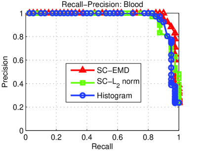
(a) Blood

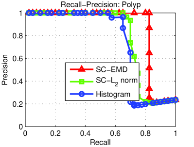
(b) Polyp

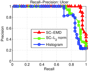
(c) Ulcer

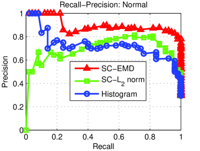
(d) Normal

Figure 1: The recall-precession curves of different classes using different histogram representation methods on the WCE images database.

The ROC curves of different classes are shown in Fig. 2. Moreover, the AUC values are given in Fig. 3. As shown in Fig. 2 and Fig. 3, our SC-EMD algorithm clearly outperforms the original histogram feature and SC-$L_{2}$ norm-based method in all four classes again. The advantage is particularly significant on the more challenging normal class. This result highlights the importance of using the EMD measure for histograms rather than $L_{2}$-norm distance.

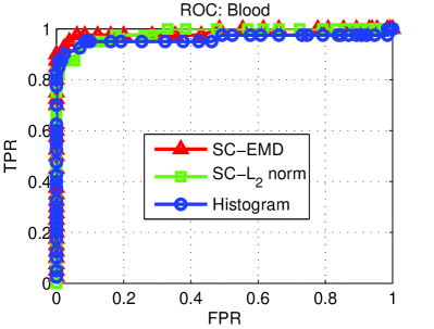
(a) Blood

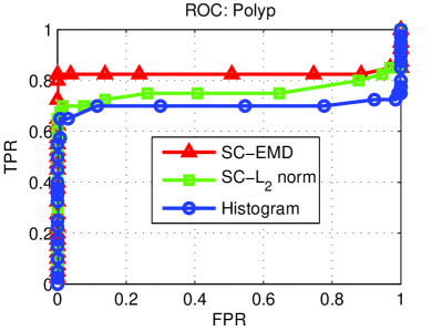
(b) Polyp

(c) Ulcer

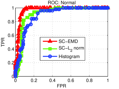
(d) Normal

Figure 2: The ROC curves of different classes using different histogram representation methods on the WCE images database.

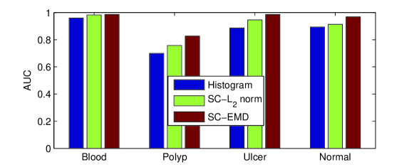
Figure 3: The AUC valuse of different classes using different histogram representation methods on the WCE images database.

3.2 Experiment II: Protein binding site retrieval

Searching geometrically similar protein binding sites is significantly important to understand the functions of protein and also to drug discovery Bind2012 ; Bradford20051487 ; Neuvirth2004181 ; Laurie20051908 . Pang et al. Bind2012 presented the protein binding sites as a histogram using the multi-instance learning framework for the protein binding site retrieval problem. In this experiment, we evaluated the proposed algorithm for the representation of histograms of protein binding sites.

3.2.1 Dataset and Setup

In this experiment, we used a protein binding site data set reported by Pang et al. Bind2012 . In this non-redundant data set, there are totally 2,819 protein binding sites, belonging to 501 different classes. The number of sites in each class varies from 2 to 58. To conduct the 4-fold cross-validation, we had selected 2,226 binding sites randomly to construct our data set. The selected data set contained sites of 249 classes, and the number of sites for each class was from 4 to 58, so that we could guarantee that when the 4-fold cross-validation was performed, in each fold there were at least one site from every class. The numbers of sites for all the selected classes are shown in Fig. 4.

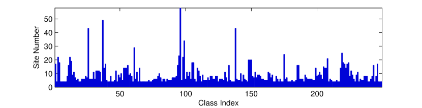
Figure 4: The numbers of sites in different classes of the protein binding site dataset.

Given a query binding site and a protein binding site database, the protein binding site retrieval problem is to rank the database sites according to their similarity to the query in a descending order, so that the database sites belonging to the same class as the query can be ranked at the top positions of the returned list. To this end, we first represented each binding site as a bag of feature points selected from the binding site surface, and for each point the geometric features were extracted Bind2012 . In the multi-instance learning framework, a binding site was refereed as a bag, and each feature point was refereed as a instance. Then all the feature points were quantized into a set of prototype points, and a histogram was generated as the bag-level feature of the binding site Bind2012 . Using the proposed SC-EMD algorithm, the histograms are represented as sparse codes for the final ranking. The ranking performances were evaluated by the recall-precision and the ROC curves. AUC values of the ROC curve were also reported as a single performance measure of the ranking results.

3.2.2 Results

The recall-precision and ROC curves of different histogram representation methods are given in Fig. 5. From the results in Fig. 5, we can find that the SC-EMD method performs the best in terms of both recall-precision and ROC curves. It proves that the EMD based method could discover the best distance measure for histogram comparison and coding. The AUC values of the ROC curves are also given in Fig. 6. These protein binding site retrieval system with SC-EMD representation method achieves an AUC value of 0.9466, compared to an AUC value of 0.9282 using SC-$L_{2}$ norm and 0.9114 using the original histogram.

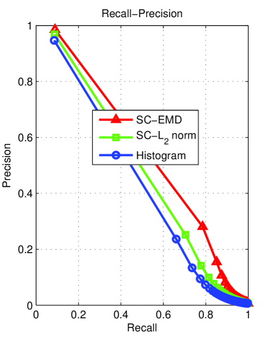
(a) Recall-Precision

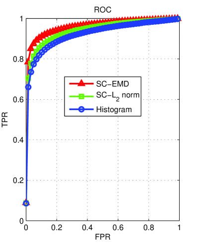
(b) ROC

Figure 5: The recall-precision and ROC curves of different histogram representation methods on the protein binding site database.

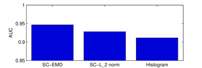
Figure 6: The AUC values of ROC curves of different histogram representation methods on the protein binding site database.

3.3 Experiment III: Object Recognition

In this section, we compared the proposed method to some other feature extraction and classification methods on an publicly accessed image database.

3.3.1 Dataset and Protocol

In this experiment, we used the COREL-2000 image database which is popular in the computer vision community for the problem of object recognition Tang2007384 ; chen2004image . In this data set, there were 2,000 images of 20 objects. For each object, the number of images was 100. The target of image recognition was to assign a given image to a class of object correctly.

To conduct the experiment, we also used the 10-fold cross-validation. Each images was regarded as a sample, and we extracted the Regions Of Interest (ROI) as the instances Christopoulos2000247 ; Heikkil2009425 . We extracted multiple ROIs for each image, thus each image was represented as a bag of multiple instances. Moreover, the instances of the training images were clustered to generate a set of instance prototypes using a clustering algorithm Frey2007972 ; Xu2005645 ; Xie1991841 ; Jain1999316 , and then the instances of each image were quantized into it to present each image as a histogram. The histograms were firstly normalized and then the proposed SC-EMD algorithm was applied to represent the histograms to sparse codes. The histogram of the training samples were used to learn the basic histograms and their sparse codes first, and then a SVM classifier was learned in the sparse code space for each class. To classify a test sample, we also represented its histogram to a sparse code vector using the basic histograms learned from the training set, and then classified the sparse code vector using the SVM classifier learned from the training set. To evaluate the classification performances of the proposed algorithm, we used the classification accuracy as the performance measure Lim2000203 ; Baldi2000412 ; Foody2002185 , which is computed as,

$$accuracy=\frac{Number~{}of~{}correctly~{}classified~{}test~{}images}{Number~{}of~{}test~{}images}.$$ (10)

3.3.2 Results

In this experiment, we compared the proposed histogram representation algorithm against several visual feature extraction methods, including the Learning Locality-Constrained Collaborative Representation (LCCR) method proposed by Peng et al. Peng2013Learning , SC-$L_{2}$, Histogram of Oriented Gradients (HOG) Suard2006206 ; Zhu20061491 ; Dalal2005886 , and Scale-Invariant Feature Transform (SIFT) Li2007332 ; Shen20091714 ; Cheung20092012 . The experiment results are given in Fig. 7 (a). As we can see from this figure, the proposed method outperforms all the other methods significantly besides LCCR. SIFT and HOG both represent the images as histograms, however, they ignore the structure of the data set by representing each images individually, thus the performances are inferior to others. SC-$L_{2}$ explorers the training set by learning a set of basic histograms to represent all the image histograms, and it achieves some minor improvements. But it uses the $L_{2}$ norm distance to compare the histograms, which is not suitable. It is very interesting to notice that LCCR, which improves the robustness and discrimination of data representation by introducing the local consistency, has archived similar performances to SC-EMD and outperformed other methods too. Although it also uses the $L_{2}$ norm as loss function which is unsuitable for histograms, it considers the local consistency of the data samples, and seek the smoothness of the code instead of the sparsity. These are the main reasons for the good performances of LCCR. It also encourages us to develop novel methods to combine EMD and locality-constrained collaborative representation, which may even improve the performance more significantly. Moreover, we also compare our method to two popular classification methods, including Sparse Representation-based Classification (SRC) Wright2009210 , Nearest Neighbor classification (NN) Zhang20062126 ; Weinberger2009207 ; Denoeux1995804 . The results is given in Fig. 7 (b). As we can see from the figure, the proposed algorithm based on EMD outperforms both the two classification using $L_{2}$ norm distance as distance metric for histograms. This is another evidence that EMD is essential for histogram data analysis and classification.

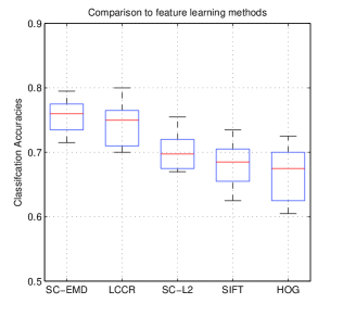
(a) Comparison to feature selection methods

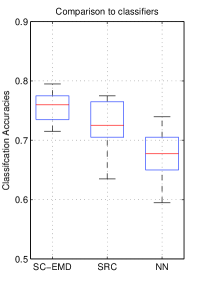
(b) Comparison to classifiers

Figure 7: Experiment results on the COREL-2000 image data set.

4 Conclusion and Future Works

A new type of sparse coding method, sparse coding with EMD metric, is proposed in this paper for the representation of histogram data. The objective function is composed of an EMD term between the original histogram and the reconstruction result from a pool of basic histograms, and a $L_{1}$ term for the regularization of the coding vector. The optimization problem is solved as a LP problem in an iterative algorithm. Algorithms based on the proposed SC-EMD outperformed previous $L_{2}$-norm based sparse coding algorithms in three challenging multi-instance learning tasks.

References

- (1) Bagby, R., Parker, J., Taylor, G.: The twenty-item toronto alexithymia scale - i: Item selection and cross-validation of the factor structure. Journal of Psychosomatic Research 38(1), 23–32 (1994)
- (2) Bai, X., Yan, C., Ren, P., Bai, L., Zhou, J.: Discriminative sparse neighbor coding. Multimedia Tools and Applications p. 25 (2015). DOI 10.1007/s11042-015-2951-4
- (3) Baldi, P., Brunak, S., Chauvin, Y., Andersen, C., Nielsen, H.: Assessing the accuracy of prediction algorithms for classification: An overview. Bioinformatics 16(5), 412–424 (2000)
- (4) Ben-Tal, A., Nemirovski, A.: Robust solutions of linear programming problems contaminated with uncertain data. Mathematical Programming, Series B 88(3), 411–424 (2000)
- (5) Bradford, J., Westhead, D.: Improved prediction of protein-protein binding sites using a support vector machines approach. Bioinformatics 21(8), 1487–1494 (2005)
- (6) Candes, E., Tao, T.: Decoding by linear programming. IEEE Transactions on Information Theory 51(12), 4203–4215 (2005)
- (7) Chen, Y., Wang, J.Z.: Image categorization by learning and reasoning with regions. The Journal of Machine Learning Research 5, 913–939 (2004)
- (8) Cherkassky, V., Ma, Y.: Practical selection of svm parameters and noise estimation for svm regression. Neural Networks 17(1), 113–126 (2004)
- (9) Cheung, W., Hamarneh, G.: n-sift: n-dimensional scale invariant feature transform. IEEE Transactions on Image Processing 18(9), 2012–2021 (2009)
- (10) Christopoulos, C., Askelöf, J., Larsson, M.: Efficient methods for encoding regions of interest in the upcoming jpeg2000 still image coding standard. IEEE Signal Processing Letters 7(9), 247–249 (2000)
- (11) Cook, N.: Use and misuse of the receiver operating characteristic curve in risk prediction. Circulation 115(7), 928–935 (2007)
- (12) Craven, P., Wahba, G.: Smoothing noisy data with spline functions - estimating the correct degree of smoothing by the method of generalized cross-validation. Numerische Mathematik 31(4), 377–403 (1978)
- (13) Dalal, N., Triggs, B.: Histograms of oriented gradients for human detection. In: Proceedings - 2005 IEEE Computer Society Conference on Computer Vision and Pattern Recognition, CVPR 2005, vol. I, pp. 886–893 (2005)
- (14) DeLong, E., DeLong, D., Clarke-Pearson, D.: Comparing the areas under two or more correlated receiver operating characteristic curves: a nonparametric approach. Biometrics 44(3), 837–845 (1988)
- (15) Denoeux, T.: -nearest neighbor classification rule based on dempster-shafer theory. IEEE Transactions on Systems, Man and Cybernetics 25(5), 804–813 (1995)
- (16) Du, X., Wang, J.Y.: Support image set machine: Jointly learning representation and classifier for image set classification. Knowledge-Based Systems 78(1), 51–58 (2015)
- (17) Ell, C., Remke, S., May, A., Helou, L., Henrich, R., Mayer, G.: The first prospective controlled trial comparing wireless capsule endoscopy with push enteroscopy in chronic gastrointestinal bleeding. Endoscopy 34(9), 685–689 (2002)
- (18) Emran, S., Ye, N.: Robustness of chi-square and canberra distance metrics for computer intrusion detection. Quality and Reliability Engineering International 18(1), 19–28 (2002)
- (19) Fan, X., Malone, B., Yuan, C.: Finding optimal bayesian network structures with constraints learned from data. In: Proceedings of the 30th Annual Conference on Uncertainty in Artificial Intelligence (UAI-14), pp. 200–209 (2014)
- (20) Fan, X., Tang, K.: Enhanced maximum auc linear classifier. In: Fuzzy Systems and Knowledge Discovery (FSKD), 2010 Seventh International Conference on, vol. 4, pp. 1540–1544. IEEE (2010)
- (21) Fan, X., Tang, K., Weise, T.: Margin-based over-sampling method for learning from imbalanced datasets. In: Advances in Knowledge Discovery and Data Mining, pp. 309–320. Springer (2011)
- (22) Fan, X., Yuan, C.: An improved lower bound for bayesian network structure learning. In: Twenty-Ninth AAAI Conference on Artificial Intelligence, pp. 2439 – 2445 (2015)
- (23) Fan, X., Yuan, C., Malone, B.: Tightening bounds for bayesian network structure learning. In: Proceedings of the 28th AAAI Conference on Artificial Intelligence, pp. 2439 – 2445 (2014)
- (24) Foody, G.: Status of land cover classification accuracy assessment. Remote Sensing of Environment 80(1), 185–201 (2002)
- (25) Frey, B., Dueck, D.: Clustering by passing messages between data points. Science 315(5814), 972–976 (2007)
- (26) Gandek, B., Ware, J., Aaronson, N., Apolone, G., Bjorner, J., Brazier, J., Bullinger, M., Kaasa, S., Leplege, A., Prieto, L., Sullivan, M.: Cross-validation of item selection and scoring for the sf-12 health survey in nine countries: Results from the iqola project. Journal of Clinical Epidemiology 51(11), 1171–1178 (1998)
- (27) Gao, S., Tsang, I.H., Chia, L.T.: Laplacian sparse coding, hypergraph laplacian sparse coding, and applications. IEEE Transactions on Pattern Analysis and Machine Intelligence 35(1), 92–104 (2013)
- (28) Gao, S., Tsang, I.H., Chia, L.T., Zhao, P.: Local features are not lonely - laplacian sparse coding for image classification. In: Proceedings of the IEEE Computer Society Conference on Computer Vision and Pattern Recognition, pp. 3555–3561 (2010)
- (29) Goadrich, M., Oliphant, L., Shavlik, J.: Gleaner: Creating ensembles of first-order clauses to improve recall-precision curves. Machine Learning 64(1-3), 231–261 (2006)
- (30) Gordon, M., Kochen, M.: Recall-precision trade-off. a derivation. Journal of the American Society for Information Science 40(3), 145–151 (1989)
- (31) Hanley, J., McNeil, B.: The meaning and use of the area under a receiver operating characteristic (roc) curve. Radiology 143(1), 29–36 (1982)
- (32) Heikkilä, M., Pietikäinen, M., Schmid, C.: Description of interest regions with local binary patterns. Pattern Recognition 42(3), 425–436 (2009)
- (33) Hershey, J., Olsen, P.: Approximating the kullback leibler divergence between gaussian mixture models. In: ICASSP, IEEE International Conference on Acoustics, Speech and Signal Processing - Proceedings, vol. 4, pp. IV317–IV320 (2007)
- (34) Huang, Y., Powers, R., Montelione, G.: Protein nmr recall, precision, and f-measure scores (rpf scores): Structure quality assessment measures based on information retrieval statistics. Journal of the American Chemical Society 127(6), 1665–1674 (2005)
- (35) Huong, V., Park, D.C., Woo, D.M., Lee, Y.: Centroid neural network with chi square distance measure for texture classification. In: Proceedings of the International Joint Conference on Neural Networks, pp. 1310–1315 (2009)
- (36) Hwang, S.: Bag-of-visual-words approach to abnormal image detection in wireless capsule endoscopy videos. Lecture Notes in Computer Science (including subseries Lecture Notes in Artificial Intelligence and Lecture Notes in Bioinformatics) 6939 LNCS(PART 2), 320–327 (2011)
- (37) Iddan, G., Meron, G., Glukhovsky, A., Swain, P.: Wireless capsule endoscopy. Nature 405(6785), 417–418 (2000)
- (38) Jain, A., Murty, M., Flynn, P.: Data clustering: A review. ACM Computing Surveys 31(3), 316–323 (1999)
- (39) Keerthi, S., Shevade, S., Bhattacharyya, C., Murthy, K.: Improvements to platt’s smo algorithm for svm classifier design. Neural Computation 13(3), 637–649 (2001)
- (40) Kotani, K., Qiu, C., Ohmi, T.: Face recognition using vector quantization histogram method. In: IEEE International Conference on Image Processing, vol. 2, pp. II/105–II/108 (2002)
- (41) Kumar, M., Gopal, M.: Reduced one-against-all method for multiclass svm classification. Expert Systems with Applications 38(11), 14,238–14,248 (2011)
- (42) Laurie, A., Jackson, R.: Q-sitefinder: An energy-based method for the prediction of protein-ligand binding sites. Bioinformatics 21(9), 1908–1916 (2005)
- (43) Lee, H., Battle, A., Raina, R., Ng, A.: Efficient sparse coding algorithms. In: Advances in Neural Information Processing Systems, pp. 801–808 (2007)
- (44) Levina, E., Bickel, P.: The earth mover’s distance is the mallows distance: Some insights from statistics. In: Proceedings of the IEEE International Conference on Computer Vision, vol. 2, pp. 251–256 (2001)
- (45) Li, L., Guo, B., Shao, K.: Geometrically robust image watermarking using scale-invariant feature transform and zernike moments. Chinese Optics Letters 5(6), 332–335 (2007)
- (46) Lim, T.S., Loh, W.Y., Shih, Y.S.: Comparison of prediction accuracy, complexity, and training time of thirty-three old and new classification algorithms. Machine Learning 40(3), 203–228 (2000)
- (47) Ling, H., Okada, K.: An efficient earth mover’s distance algorithm for robust histogram comparison. IEEE Transactions on Pattern Analysis and Machine Intelligence 29(5), 840–853 (2007)
- (48) Liu, Y., Ding, M.F.: A ladder method for linear semi-infinite programming. Journal of Industrial and Management Optimization 10(2), 397–412 (2014)
- (49) Liu, Y., Zheng, Y.: One-against-all multi-class svm classification using reliability measures. In: Proceedings of the International Joint Conference on Neural Networks, vol. 2, pp. 849–854 (2005)
- (50) Lu, Z.M., Burkhardt, H.: Colour image retrieval based on dct-domain vector quantisation index histograms. Electronics Letters 41(17), 956–957 (2005)
- (51) Mairal, J., Bach, F., Ponce, J., Sapiro, G.: Online learning for matrix factorization and sparse coding. Journal of Machine Learning Research 11, 19–60 (2010)
- (52) Mylonaki, M., Fritscher-Ravens, A., Swain, P.: Wireless capsule endoscopy: A comparison with push enteroscopy in patients with gastroscopy and colonoscopy negative gastrointestinal bleeding. Gut 52(8), 1122–1126 (2003)
- (53) Neuvirth, H., Raz, R., Schreiber, G.: Promate: A structure based prediction program to identify the location of protein-protein binding sites. Journal of Molecular Biology 338(1), 181–199 (2004)
- (54) Pang, B., Zhao, N., Korkin, D., Shyu, C.R.: Fast protein binding site comparisons using visual words representation. Bioinformatics 28(10), 1345–1352 (2012)
- (55) Pencina, M., D’Agostino Sr., R., D’Agostino Jr., R., Vasan, R.: Evaluating the added predictive ability of a new marker: From area under the roc curve to reclassification and beyond. Statistics in Medicine 27(2), 157–172 (2008)
- (56) Peng, X., Zhang, L., Yi, Z., Tan, K.K.: Learning locality-constrained collaborative representation for robust face recognition. Pattern Recognition 47(9), 2794–2806 (2014)
- (57) Polat, K., Gunes, S.: A novel hybrid intelligent method based on c4.5 decision tree classifier and one-against-all approach for multi-class classification problems. Expert Systems with Applications 36(2 PART 1), 1587–1592 (2009)
- (58) Rached, Z., Alajaji, F., Campbell, L.: The kullback-leibler divergence rate between markov sources. IEEE Transactions on Information Theory 50(5), 917–921 (2004)
- (59) Rubner, Y., Tomasi, C., Guibas, L.: Earth mover’s distance as a metric for image retrieval. International Journal of Computer Vision 40(2), 99–121 (2000)
- (60) Sandler, R., Lindenbaum, M.: Nonnegative matrix factorization with earth mover’s distance metric for image analysis. Pattern Analysis and Machine Intelligence, IEEE Transactions on 33(8), 1590–1602 (2011)
- (61) Schüldt, C., Laptev, I., Caputo, B.: Recognizing human actions: A local svm approach. In: Proceedings - International Conference on Pattern Recognition, vol. 3, pp. 32–36 (2004)
- (62) Seghouane, A.K., Amari, S.I.: The aic criterion and symmetrizing the kullback-leibler divergence. IEEE Transactions on Neural Networks 18(1), 97–106 (2007)
- (63) Shen, Y., Guturu, P., Damarla, T., Buckles, B., Namuduri, K.: Video stabilization using principal component analysis and scale invariant feature transform in particle filter framework. IEEE Transactions on Consumer Electronics 55(3), 1714–1721 (2009)
- (64) Suard, F., Rakotomamonjy, A., Bensrhair, A., Broggi, A.: Pedestrian detection using infrared images and histograms of oriented gradients. In: IEEE Intelligent Vehicles Symposium, Proceedings, pp. 206–212 (2006)
- (65) Tang, J., Lewis, P.: A study of quality issues for image auto-annotation with the corel dataset. IEEE Transactions on Circuits and Systems for Video Technology 17(3), 384–389 (2007)
- (66) Tsai, P.: Histogram-based reversible data hiding for vector quantisation-compressed images. IET Image Processing 3(2), 100–114 (2009)
- (67) Tsang, I., Kwok, J., Cheung, P.M.: Core vector machines: Fast svm training on very large data sets. Journal of Machine Learning Research 6 (2005)
- (68) Wang, J., Zhou, Y., Yin, M., Chen, S., Edwards, B.: Representing data by sparse combination of contextual data points for classification. In: X. Hu, Y. Xia, Y. Zhang, D. Zhao (eds.) Advances in Neural Networks ?ISNN 2015, Lecture Notes in Computer Science, vol. 9377, pp. 373–381 (2015)
- (69) Weinberger, K., Saul, L.: Distance metric learning for large margin nearest neighbor classification. Journal of Machine Learning Research 10, 207–244 (2009)
- (70) Wright, J., Yang, A., Ganesh, A., Sastry, S., Ma, Y.: Robust face recognition via sparse representation. IEEE Transactions on Pattern Analysis and Machine Intelligence 31(2), 210–227 (2009)
- (71) Xie, X.L., Beni, G.: A validity measure for fuzzy clustering. IEEE Transactions on Pattern Analysis and Machine Intelligence 13(8), 841–847 (1991)
- (72) Xu, R., Wunsch II, D.: Survey of clustering algorithms. IEEE Transactions on Neural Networks 16(3), 645–678 (2005)
- (73) Yang, J., Ding, Z., Guo, F., Wang, H., Hughes, N.: A novel multivariate performance optimization method based on sparse coding and hyper-predictor learning. Neural Networks 71, 45–54 (2015)
- (74) Yang, J., Yu, K., Gong, Y., Huang, T.: Linear spatial pyramid matching using sparse coding for image classification. In: 2009 IEEE Computer Society Conference on Computer Vision and Pattern Recognition Workshops, CVPR Workshops 2009, pp. 1794–1801 (2009)
- (75) Ye, N., Parmar, D., Borror, C.: A hybrid spc method with the chi-square distance monitoring procedure for large-scale, complex process data. Quality and Reliability Engineering International 22(4), 393–402 (2006)
- (76) Zhang, H., Berg, A., Maire, M., Malik, J.: Svm-knn: Discriminative nearest neighbor classification for visual category recognition. In: Proceedings of the IEEE Computer Society Conference on Computer Vision and Pattern Recognition, vol. 2, pp. 2126–2136 (2006)
- (77) Zheng, M., Bu, J., Chen, C., Wang, C., Zhang, L., Qiu, G., Cai, D.: Graph regularized sparse coding for image representation. IEEE Transactions on Image Processing 20(5), 1327–1336 (2011)
- (78) Zhou, Z.H., Jiang, K., Li, M.: Multi-instance learning based web mining. Applied Intelligence 22(2), 135–147 (2005)
- (79) Zhou, Z.H., Sun, Y.Y., Li, Y.F.: Multi-instance learning by treating instances as non-i.i.d. samples. In: Proceedings of the 26th International Conference On Machine Learning, ICML 2009, pp. 1249–1256 (2009)
- (80) Zhou, Z.H., Zhang, M.L.: Multi-instance multi-label learning with application to scene classification. In: Advances in Neural Information Processing Systems, pp. 1609–1616 (2007)
- (81) Zhu, Q., Avidan, S., Yeh, M.C., Cheng, K.T.: Fast human detection using a cascade of histograms of oriented gradients. In: Proceedings of the IEEE Computer Society Conference on Computer Vision and Pattern Recognition, vol. 2, pp. 1491–1498 (2006)