Determination of Tomonaga-Luttinger parameters for a two-component liquid

We provide evidence for the mapping of critical spin-1 chains, in particular the $\mathrm{SU}(3)$ symmetric bilinear-biquadratic model with additional interactions, to free boson theories using exact diagonalization and the density matrix renormalization group algorithm. Using the correspondence with a conformal field theory with central charge $c=2$, we determine the analytic formulae for the scaling dimensions in terms of four Tomonaga-Luttinger liquid parameters. By matching the lowest scaling dimensions, we numerically calculate these field-theoretic parameters and track their evolution as a function of the parameters of the lattice model.

I Introduction

Given a strongly correlated quantum system, an important step towards understanding it is to determine its basic properties, such as the presence or absence of a gap, the presence of spontaneous symmetry breaking, etc. One then asks for more specific information, and ultimately, the complete description of the underlying low-energy physics. Quite often, this characterization involves determining an effective field theory. Examples include topological field theories describing the full braiding statistics in gapped quantum systems, and conformal field theories (CFT), describing the set of independent critical exponents in gapless systems. Obtaining these conformal exponents is important because close to the critical point, the power law behavior of physical quantities like magnetic susceptibility is governed by them. These dimensions complement the knowledge of the central charge, denoted by $c$, in determining the universal long-distance behavior of the theory.

In recent times, several probes, such as the entanglement entropy (EE), Renyi entropies and entanglement spectrum Calabrese_Cardy ; Li_Haldane ; Ryu ; Headrick ; Tubman ; Melko ; Ryu_Hatsugai ; Thomale2010 ; Lundgren2014 , have been devised to explore the above mentioned properties. A central component of all these measures is the ground state reduced density matrix, calculated for a finite region of space and obtained by tracing the full density matrix over the other degrees of freedom. For example, the finite-size scaling of the EE in one-dimensional critical systems provides a precise estimate of the central charge of the corresponding CFT. More sophisticated ways of using reduced density matrices also reveal information about the low-energy scaling dimensions and operators Cheong_Henley ; Muender ; Henley_Changlani ; Melko_mutual ; Barcza ; Furukawa2009 .

For one dimensional (1D) critical systems, the theory of Tomonaga-Luttinger liquids (TLLs) Tomonaga ; Luttinger_original ; Giamarchi ; Haldane_Luttinger has been remarkably successful at characterizing their low-energy physics. There has been additional validation on the experimental front, at least qualitatively; several realizations, ranging from carbon nanotubes Bockrath ; Ishii to semiconductor wires Yacoby , of TLL physics have been found. Quantitative estimates of the scaling dimensions, velocity, and Luttinger parameter for model Hamiltonians have been made with analytic solutions or numerically, with exact diagonalization and density matrix renormalization group dmrg_white methods Lauchli_operator ; Jeckelmann_DMRG ; Karrasch ; Dalmonte ; Furukawa2009 .

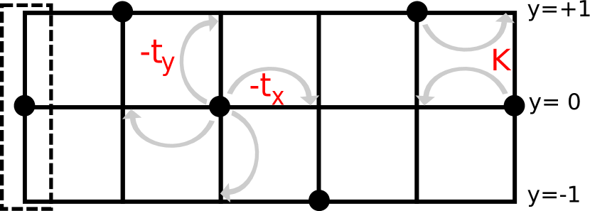
Figure 1: A representative configuration of hard-core bosons on a three leg ladder with periodic boundary conditions in the transverse or rung direction, with Hamiltonian given by Eq. (1a). The hopping in the length ($t_{x}$) and transverse ($t_{y}$) directions respectively and the correlated hop ($K$) on the square plaquette have been indicated by arrows. For $t_{x}=0$ and at 1/3 filling, the low energy model involves configurations with only with exactly one boson per rung. The three configurations per rung, one of which has been enclosed in a dotted rectangle, when appropriately Fourier transformed, are mapped to a spin-1 basis. The resultant spin-1 Hamiltonian has the form Eq. (2a)

Most theoretical studies have focused on the single component TLL, which directly corresponds to a $c=1$ CFT, and which now appears to be a fairly well understood case Giamarchi ; Furukawa2009 . In contrast, there are few general results for the $c=2$ case, despite the existence of systems with this property Rex_TLL ; Sakai . This is partly attributed to the TLL theory for $c=1$ being completely described by a single dimensionless parameter, whereas the $c=2$ theory requires four dimensionless parameters. An important open question is that there is no established method to extract TLL parameters for a given lattice model. Given the history of the TLL, it appears to us that this situation is quite unsatisfactory and incomplete.

In special cases, a $c=2$ CFT can be understood as a tensor product of two $c=1$ CFTs; for example, the 1D Hubbard model has two TLL parameters, one for spin and the other for charge. In this paper, however, we will demonstrate a TLL parameter extraction procedure for a $c=2$ CFT where such a decomposition does not apply. Several conceptual and practical questions arise here; including which measures must be calculated to estimate them and whether they are numerically accurate enough to validate or refute a given field theory. Our paper addresses these questions and highlights an interesting application of relatively new ground state entanglement based metrics, such as the mutual information. However, before considering a specific problem to demonstrate our ideas for $c=2$ CFTs, we mention physical examples where this situation occurs.

One way to realize a multi-component TLL is to couple several TLLs Schulz1 ; Schulz2 . The most natural geometry for doing this is a ladder (or tube), a quasi-one dimensional system made up of one dimensional legs which are additionally coupled in the transverse or rung direction, with open (or periodic) boundary conditions. Fig. 1 shows an example with three legs, relevant for modelling quasi one-dimensional compounds such as [(CuCl₂tachH)₃Cl]Cl₂ Schnack and CsCrF₄ Manaka , and to which recent theoretical works Bose_metal ; Balents_spin_tube ; Sakai ; Sato_PRB have been devoted.

Following the work of Ref. Bose_metal and as is schematically depicted in Fig. (1), our starting point is a system of hard-core bosons on a three leg tube, governed by the Hamiltonian,

$$H = H_{\text{hop}}+H_{K}$$ (1a)

$$H_{\text{hop}} = -t_{x}\sum_{{\bf r}}b_{{\bf r}}^{\dagger}b_{{\bf r}+\hat{x}}+\text{h.c.}-t_{y}\sum_{{\bf r}}b_{{\bf r}}^{\dagger}b_{{\bf r}+\hat{y}}+\text{h.c.}$$ (1b)

$$H_{K} = K\sum_{{\bf r}}b_{{\bf r}}^{\dagger}b_{{\bf r}+\hat{x}}b_{{\bf r}+\hat{x}+\hat{y}}^{\dagger}b_{{\bf r}+\hat{y}}+\text{h.c.}$$ (1c)

where $t_{y}$ and $t_{x}$ are the hoppings along the transverse ($y$) and length ($x$) directions respectively, $K$ is a correlated exchange on a square plaquette. The phase diagram of this model is expected to be quite rich; here we only consider the case of $t_{x},t_{y}\rightarrow 0$ with 1/3 filling of bosons. In this parameter regime, the low-energy theory of this model involves only one boson per rung (column) allowing three distinct states on it; the number per rung can not change because of the absence of hopping in the $x$ direction.

On Fourier transforming bosonic creation operators along the $y$ direction, a new basis at every $x$ location is defined as, $|0\rangle_{x}\equiv\frac{1}{\sqrt{3}}\left(b_{x,0}^{\dagger}+b_{x,1}^{\dagger}+b_{x,-1}^{\dagger}\right)|vac\rangle$ and $|\pm\rangle_{x}\equiv\frac{1}{\sqrt{3}}\left(b_{x,0}^{\dagger}+\omega b_{x,\pm 1}^{\dagger}+\omega^{2}b_{x,\mp 1}^{\dagger}\right)|vac\rangle$ where $\omega=\exp\left(i2\pi/3\right)$. The three components can be thought of as those corresponding to a pseudospin-1 object, leading to the effective spin-Hamiltonian of the form Bose_metal ,

$${H} = K\Big{(}\sum_{\langle ij\rangle}{\mathbf{S}_{i}\cdot{\mathbf{S}_{j}}}+\sum_{\langle ij\rangle}\left({\mathbf{S}_{i}}\cdot{\mathbf{S}_{j}}\right)^{2}\Big{)}+Q_{x}+Q_{y}$$ (2a)

$$Q_{x(y)} = q_{x(y)}\sum_{i}{U_{x(y)}^{\dagger i}U^{i+1}_{x(y)}}+\text{h.c.}$$ (2b)

where $\mathbf{S}_{i}$ is a spin-1 operator living on site $i$, while $q_{x}$ and $q_{y}$ are scalars. $K$ will be set to $1$ throughout and thus all energy scales in this paper are in terms of this unit. $U_{x}$ and $U_{y}$ are $3\times 3$ matrices in the $S_{z}$ basis (ordered as $-1,0,1$), and are given by,

$$U_{x}=\left(\begin{array}[]{ccc}\omega^{-1}&0&0\\ 0&1&0\\ 0&0&\omega\end{array}\right),\quad U_{y}=\left(\begin{array}[]{ccc}0&0&1\\ 1&0&0\\ 0&1&0\end{array}\right),$$ (9)

The $Q_{y}$ term is non-zero with $q_{y}=-1/3$, but there is no $Q_{x}$ term i.e. $q_{x}=0$. Physically, the term $U^{i,\dagger}_{y}U^{j}_{y}$ models a correlated cyclic permutation of neighboring spins. However, diagonalizing $U_{y}$, i.e. performing a similarity transformation by the matrix,

$$S=\frac{1}{\sqrt{3}}\left(\begin{array}[]{ccc}\omega^{-1}&\omega&1\\ 1&1&1\\ \omega&\omega^{-1}&1\end{array}\right),$$ (13)

preserves the combined $\mathbb{SU}(3)$ symmetry of the first two terms in (2a) and converts the $Q_{y}$ term into the $Q_{x}$ term because $SU_{y}S^{\dagger}=U_{x}$. For presentational purposes, we have shown both terms in Eq. (2a); this generalized model has been previously introduced in the literature as the quantum torus chain Qin_torus .

For $q_{x}=q_{y}=0$, this model is the analytically solvable Lai-Sutherland model Lai ; Sutherland ; Itoi_Kato , which serves as a useful guide for checking our calculations. Since $Q_{x}$ and $Q_{y}$ are related by a $\mathrm{SU(3)}$ unitary transformation; studying the model with $q_{x}$ non zero and $q_{y}=0$ is equivalent to the case with $q_{x}=0$ and $q_{y}$ non-zero. We set $q_{y}=0$ throughout this paper, and leave the more general case for later exploration. Finally, we note that a generalized version is the bilinear-biquadratic model Papa , whose phase-diagram includes a gapless phase and the gapped Haldane phase Haldane ; AKLT and which has been experimentally realized in LiVGe₂O₆ Millet_expt .

We now discuss the organization of the remainder of the paper. In Sec. II, we discuss how the low-energy theory of the spin-1 model (2a), motivated above, is mapped to a field theory using bosonization techniques. We then develop the analytic formulas for the scaling dimensions of the low-energy theory in terms of the TLL parameters: these formulae are generalizations of those known for the $c=1$ case Oshikawa_TLL . For the particular case of parameters of the spin-1 Hamiltonian (2a) ($q_{x}>0$, $q_{y}=0$), these formulae show the explicit dependence of the TLL parameters on the microscopic model parameter. In Sec. III, we provide numerical evidence for the connection between the low energy theory of the spin chain and the CFT for $c=2$, by calculating the lowest two scaling dimensions with exact diagonalization (ED) and the density matrix renormalization group (DMRG). The TLL parameters obtained are tracked as a function of the microscopic parameter $q_{x}$. Finally in Sec. IV, we conclude by discussing generalizations of our method and the prospective applications to other systems.

II Mapping Spin-1 Lattice models to free boson theory

II.1 Symmetries

In this section, we develop a continuum field theory description for the lattice Hamiltonian (2a), by closely following Refs. Affleck_Les ; Itoi_Kato , wherein more details are spelled out. For a start, symmetry properties of the Hamiltonian (2a) are described here piece by piece. To this end, the spin-1 part of the Hamiltonian (2a) can be written (up to a constant factor) in a manifestly $\mathrm{SU(3)}$ symmetric way in terms of $3\times 3$ elementary matrices $L^{\alpha}_{\beta}$ with one on row $\alpha$ and column $\beta$ and zero everywhere else as

$${H}_{\text{SU(3)}}=\sum_{\langle ij\rangle}\sum_{\alpha,\beta=0,1,2}L^{\alpha}_{\,\beta\,i}L^{\beta}_{\,\alpha\,j}.$$ (14)

For convenience, this Hamiltonian can be represented in terms of fermionic operators using $L^{\alpha}_{\,\beta\,i}=c^{\alpha\dagger}_{i}c_{\beta\,i}$, with the constraint $\sum_{\alpha=0,1,2}c^{\alpha\dagger}_{i}c_{\alpha\,i}=\sum_{\alpha=0,1,2}n_{\alpha i}=1$ at each site $i$. The constraint ensures that the operators have the same commutation (anticommutation) relations and act on Hilbert spaces of the same dimensions. The Hamiltonian $H_{\mathrm{SU(3)}}$ conserves the particle numbers $N_{1}-N_{0}$ and $N_{2}-N_{0}$, where $N_{\alpha}=\sum_{i}c^{\alpha{\dagger}}_{i}c_{\alpha i}$. Defining the dual basis by $\tilde{c}_{n}={3}^{-1/2}\sum_{\alpha=0}^{2}{c}_{\alpha}w^{n}$ for $n=0,1,2$, and the corresponding particle numbers as $\tilde{N}_{n}=\sum_{i}\tilde{c}^{n{\dagger}}_{i}\tilde{c}_{ni}$, the Hamiltonian $H_{\mathrm{SU(3)}}$ also conserves the dual particle numbers $\tilde{N}_{1}-\tilde{N}_{0}$ and $\tilde{N}_{2}-\tilde{N}_{0}$.

On the other hand, the $Q_{x}$ perturbation in (2a) can be written as

$$Q_{x}=3q_{x}\sum_{i,\alpha}L^{\alpha}_{\alpha\,i}L^{\alpha}_{\alpha\,i+1}.$$ (15)

The Hamiltonian $H_{\mathrm{SU(3)}}+Q_{x}$ conserves the particle numbers $N_{1}-N_{0}$ and $N_{2}-N_{0}$, and it conserves the dual particle numbers $\tilde{N}_{1}-\tilde{N}_{0}$ and $\tilde{N}_{2}-\tilde{N}_{0}$ (mod 3).

II.2 Continuum theory

The low-energy effective field theory for the Hamiltonian $H_{\mathrm{SU(3)}}$ can be developed by noting that at low energies, only excitations close to the Fermi points $k_{F}=\pi/3a_{0}$ (where $a_{0}$ is the lattice constant) propagate. Thus we can approximate,

$$c_{\alpha\,i}\approx\sqrt{a_{0}}[e^{ik_{F}x_{i}}\psi_{R\alpha}(x_{i})+e^{-ik_{F}x_{i}}\psi_{L\alpha}(x_{i})].$$ (16)

Substituting this in the Hamiltonian and dropping oscillatory terms, the low energy theory can be written in terms of the $U(3)$ currents,

$$J_{R,L\,\beta}^{\alpha}=\psi_{R,L}^{\alpha\dagger}\psi_{R,L\,\beta},$$ (17)

as

$${H}_{\text{SU(3)}}=\pi v_{F}\int dx\sum_{\alpha,\beta}[J_{R\,\beta}^{\alpha}J_{R\,\alpha}^{\beta}+J_{L\,\beta}^{\alpha}J_{L\,\alpha}^{\beta}+2J_{R\,\beta}^{\alpha}J_{L\,\alpha}^{\beta}$$

$$\qquad-2\cos(2k_{F}a_{0})J_{R\,\alpha}^{\alpha}J_{L\,\beta}^{\beta}],$$ (18)

where $v_{F}$ is the Fermi velocity, which will be set to 1 henceforth. The last term depends only on the charged modes, $J^{\alpha}_{R\alpha}$ and $J^{\alpha}_{L\alpha}$, which are gapped, while the second term can be shown to be marginally irrelevant in the RG sense. While this term must be retained to evaluate quantitative finite size logarithmic corrections, here we simplify the analysis by working directly in the conformal limit. Instead, the finite size corrections will be reintroduced only at a later stage, when comparing the analytic results with numerical calculations. Thus, with this simplification, the critical theory is,

$${H}_{\text{SU(3)}}\approx{H}_{\mathrm{WZW}}=\pi\int dx\sum_{\alpha,\beta}[J_{R\,\beta}^{\alpha}J_{R\,\alpha}^{\beta}+J_{L\,\beta}^{\alpha}J_{L\,\alpha}^{\beta}].$$ (19)

We note that this is a $U(3)$ Wess-Zumino-Witten (WZW) model and thus contains an $\mathrm{SU(3)}_{1}$ and $U(1)$ part yellowbook . The $U(1)$ piece is precisely the charged mode which is gapped and will be dropped later. (N.B. the above procedure is better described and applied, instead of dealing with the $\mathrm{SU(3)}$ Lai-Sutherland model, by starting with the Hubbard type model $H=-t\sum_{\langle ij\rangle\alpha}[c^{{\dagger}}_{i\alpha}c^{\ }_{j\alpha}+h.c.]+U\sum_{i,\alpha\neq\beta}n_{i\alpha}n_{i\beta}$ without constraint $\sum_{\alpha}n_{\alpha i}=1$. This constraint is in fact generated dynamically and this model reduces to the $\mathrm{SU(3)}$ symmetric spin model when expanded in $t/U$.)

Applying the same reasoning as above one deduces the continuum approximation

$$Q_{x}\approx 3q_{x}\int dx\sum_{\alpha}\left[(J_{R\,\alpha}^{\alpha})^{2}+(J_{L\,\alpha}^{\alpha})^{2}\right],$$ (20)

where again we have dropped the terms that only depend on the charged mode.

II.3 Abelian Bosonization

Introducing holomorphic and antiholomorphic coordinates for 1+1 d space-time $z=-i(x-t)$, and $\bar{z}=i(x+t)$, the time evolution of the fields factorize nicely so that the fields with an $R(L)$ subscript depend only on $z(\bar{z})$ respectively. The continuum Fermi fields in Eq. (16) can be bosonized as follows

$$\psi^{\ }_{\beta L}=\frac{1}{2\pi a_{0}}:e^{-i\sqrt{4\pi}\phi_{\beta L}}:,\quad\psi^{\beta\dagger}_{L}=\frac{1}{2\pi a_{0}}:e^{i\sqrt{4\pi}\phi_{\beta L}}:,$$ (21)

where $\phi_{L}$ represents the holomorphic part of a free boson field. We focus on the holomorphic parts of the theory (dropping the L subscript) with similar formulae for left moving fermions in terms of the anti-holomorphic part of the free boson field. We have introduced normal ordering of an operator $O$, denoted by $:O:$, which must be used when two fields at the same point are multiplied together. Usually when bosonizing more that one species of fermions, one introduces Klein factors to ensure that different Fermi fields anticommute. These Klein factors have been ignored here since they are not dynamical and do not play a role in the Hamiltonian which is mainly what we are interested in here.

A key identity, which can be regarded as the inverse of Eq. (21), is

$$\psi^{\alpha\dagger}\psi^{\ }_{\alpha}(z)=\frac{-i}{\sqrt{\pi}}\partial\phi_{\alpha}(z),$$ (22)

where $\partial$ denotes a derivative with respect to $z$. To understand the split into $\mathrm{SU(3)}$ and $\mathrm{U(1)}$ WZW theories mentioned above we introduce the $\mathrm{SU(3)}$ and $\mathrm{U(1)}$ currents given by

$$J^{a}=\sum_{\alpha,\beta}\psi^{\alpha\dagger}T^{a}_{\alpha\beta}\psi_{\beta},\quad J=\sum_{\alpha}\psi^{\alpha\dagger}\psi^{\ }_{\alpha},$$ (23)

where $T^{a}$ are generators of the $\mathrm{SU(3)}$ algebra. The $U(1)$ piece in the boson language satisfies

$$J=\frac{-i}{\sqrt{\pi}}\left(\partial\phi_{0}+\partial\phi_{1}+\partial\phi_{2}\right).$$ (24)

The $\mathrm{SU(3)}$ currents associated to the Cartan sub-algebra are

$$H^{1} \propto\psi^{0\dagger}\psi_{0}-\psi^{1\dagger}\psi_{1}\propto\partial\phi_{0}-\partial\phi_{1},$$

$$H^{2} \propto\psi^{0\dagger}\psi_{0}+\psi^{1\dagger}\psi_{1}-2\psi^{2\dagger}\psi_{2}\propto\partial\phi_{0}+\partial\phi_{1}-2\partial\phi_{2}.$$ (25)

So we can make an operator product expansion (OPE) preserving orthogonal change of basis to introduce $\tilde{\phi}_{0,1,2}$ as

$$\tilde{\phi}_{0} =(\phi_{0}+\phi_{1}+\phi_{2})/\sqrt{3},$$ (26)

$$\tilde{\phi}_{1} =(\phi_{0}-\phi_{1})/\sqrt{2},$$

$$\tilde{\phi}_{2} =(\phi_{0}+\phi_{1}-2\phi_{2})/\sqrt{6}.$$

In this basis the dynamics of the charged mode is now encoded in the single boson field $\tilde{\phi}_{0}$. Therefore dropping the charged mode corresponds to setting $\tilde{\phi}_{0}=0$. This is indicated with an arrow in the equations below. In this basis some of the $\mathrm{SU(3)}$ currents associated with the Cartan subalgebra are simply (up to a constant factor) $\partial\tilde{\phi}_{1}$, $\partial\tilde{\phi}_{2}$, while those associated with a choice of simple roots for $\mathrm{SU(3)}$ are

$$J^{\boldsymbol{\alpha}_{1}} \propto\psi_{0}^{\dagger}\psi_{1}\propto e^{i\sqrt{4\pi}(\phi_{1}-\phi_{0})}\rightarrow e^{i\sqrt{8\pi}\boldsymbol{\alpha}_{1}\cdot\tilde{\boldsymbol{\phi}}},$$

$$J^{\boldsymbol{\alpha}_{2}} \propto\psi_{0}^{\dagger}\psi_{2}\propto e^{i\sqrt{4\pi}(\phi_{2}-\phi_{0})}\rightarrow e^{i\sqrt{8\pi}\boldsymbol{\alpha}_{2}\cdot\tilde{\boldsymbol{\phi}}}.$$

$\boldsymbol{\alpha}_{1}$ and $\boldsymbol{\alpha}_{2}$ together with a third root $\boldsymbol{\alpha}_{3}$ are given by,

$$\boldsymbol{\alpha}_{1}=(1,0),\,\boldsymbol{\alpha}_{2}=\left(\frac{1}{2},\frac{\sqrt{3}}{2}\right),\,\boldsymbol{\alpha}_{3}=\left(\frac{1}{2},-\frac{\sqrt{3}}{2}\right).$$ (27)

All other roots of $\mathrm{SU(3)}$ can be obtained as integer linear combinations of $\boldsymbol{\alpha}_{1}$ and $\boldsymbol{\alpha}_{2}$, for example $\boldsymbol{\alpha}_{3}=\boldsymbol{\alpha}_{1}-\boldsymbol{\alpha}_{2}$. Similarly, the vertex operators associated with all other roots can be obtained from operator products of $J^{\boldsymbol{\alpha}_{1}}$ and $J^{\boldsymbol{\alpha}_{2}}$. This construction gives precisely the vertex operators obtained in the purely bosonic construction of $\mathrm{SU(3)}_{1}$ where the boson fields $\tilde{\phi}_{1}$ and $\tilde{\phi}_{2}$ are compactified on the root lattice of the $\mathrm{SU(3)}$ algebra GSW . All proportionality constants can be fixed by a choice of normalization of the $\mathrm{SU(3)}$ generators.

We now obtain the purely bosonic description of the gapless degrees of freedom of the spin-1 chain. The key identities are

$$\sum_{\alpha}J^{\alpha}_{\alpha}J^{\alpha}_{\alpha} =-\sum_{\alpha}\partial\phi_{\alpha}\partial\phi_{\alpha}$$

$$\rightarrow-(\partial\tilde{\phi}_{1}\partial\tilde{\phi}_{1}+\partial\tilde{\phi}_{2}\partial\tilde{\phi}_{2}),$$ (28)

$$\sum_{\alpha\neq\beta}J^{\alpha}_{\beta}J^{\beta}_{\alpha} =-\sum_{\alpha\neq\beta}\partial\phi_{\alpha}\partial\phi_{\beta}$$

$$\rightarrow-(\partial\tilde{\phi}_{1}\partial\tilde{\phi}_{1}+\partial\tilde{\phi}_{2}\partial\tilde{\phi}_{2}).$$ (29)

Using these, we obtain the main results of this section

$$H_{\mathrm{SU(3)}}\approx-2\int dx(\partial\phi_{1}\partial\phi_{1}+\partial\phi_{2}\partial\phi_{2}+\text{antilhol}),$$

$$Q_{x}\approx-3q_{x}\int dx(\partial\phi_{1}\partial\phi_{1}+\partial\phi_{2}\partial\phi_{2}+\text{antilhol}).$$ (30)

where antihol denotes the antiholomorphic part. Note that the tildes have now been dropped: the effective Hamiltonian of the spin-1 chain is now written in terms of $\mathrm{SU(3)}_{1}$ boson fields $\phi_{1}$ and $\phi_{2}$. We note that these quantities are all non-negative since we have for any field $\phi$,

$$\partial\phi\partial\phi+\bar{\partial}\phi\bar{\partial}\phi=-\frac{1}{2}\left(\partial_{x}\phi\partial_{x}\phi+\partial_{t}\phi\partial_{t}\phi\right).$$ (31)

II.4 General $c=2$ Boson theories

In the previous section, we derived the low-energy effective Hamiltonian that should capture the critical dynamics of the spin-1 chain with the $Q_{x}$ perturbation. The low-energy effective theory consists of two compactified boson fields and has the central charge $c=2$. To put the effective theory in a general context, we discuss in this subsection a generic two-component boson theory with $c=2$.

For the case of the single-component TLL, the landscape of the theory (often called “moduli space”) is well understood. It is characterized solely by a single parameter, the Luttinger parameter $K$ or the compactification radius $R$ of the boson field. There is a boson-vortex duality in (1+1)d (also known as “T-duality”) which relates the two regions $K>1$ and $K<1$. These regions are separated by the self-dual point $K=1$ where $\mathrm{SU(2)}$ symmetry is realized. With orbifolding, theory space for $c=1$ is described in terms of two axis, each describing the ordinary free boson theory (the single-component TLL) and its orbifolded counterpart, together with a few “exceptional cases” Ginsparg_Les .

On the other hand, the moduli space for the $c=2$ theories is more complicated. For a start, let us consider the action in 1+1 d space-time for two bosonic fields $X^{1,2}$,

$$S=\frac{1}{4\pi}\int dxdt\,(G_{ab}\partial_{\mu}X^{a}\partial_{\mu}X^{b}+B_{ab}\epsilon_{\mu\nu}\partial_{\mu}X^{a}\partial_{\nu}X^{b}),$$ (32)

where $\mu,\nu=0,1$, and $G$ and $B$ are a symmetric (non degenerate) and antisymmetric 2 by 2 real matrix, respectively.

$$X^{a}\sim X^{a}+2\pi.$$ (33)

The corresponding Hamiltonian is given by,

$${H}=-\frac{1}{2\pi}\int dx\,G_{ab}(\partial X^{a}\partial X^{b}+\text{antihol}),$$ (34)

Observe that the parameter $B$ does not enter into the Hamiltonian: it is a topological term. However, it affects the canonical commutation relations and hence the spectrum.

There are thus four independent parameters, $G_{11},G_{12},G_{22}$ and $B_{12}$, characterizing the $c=2$ action (32), as opposed to the $c=1$ TLL parameterized by a single parameter. (As in the case of $c=1$, one can consider various orbifolds of the two-component boson theory (32), leading to an even richer moduli space or phase diagram Dulat . )

For the case of $c=1$ TLL, the duality relates the large and small compactification radius (the Luttinger parameter). Similarly, there is a group of duality transformations acting on the four parameters, and different values of $G$ and $B$ do not necessarily correspond to different spectra  becker2006string ; Giveon . To unveil this duality group, it is convenient to trade the four real parameters in $G$ and $B$ for two complex parameters $\xi$ and $\rho$ as follows

$$\xi\equiv\frac{G_{12}}{G_{22}}+i\frac{\sqrt{\text{det}\,G}}{G_{22}},$$

$$\rho\equiv B_{12}+i\sqrt{\det\,G}.$$ (35)

These two parameters can be acted upon by independent $SL(2,\mathbb{Z})$ transformations which for $\xi$ is given by

$$\xi\rightarrow\frac{a\xi+b}{c\xi+d},$$ (36)

where $a,b,c,d\in\mathbb{Z},ad-bc=1$. There is a similar independent transformation for $\rho$. These transformations change the parameters $G$ and $B$ but lead to the same spectrum. Effectively the target space of the boson fields corresponds to two tori, which are left invariant by $SL(2,\mathbb{Z})\times SL(2,\mathbb{Z})$ transformations. There are two further discrete transformations that leave the spectrum invariant:

$$(\xi,\rho)\rightarrow(\rho,\xi),\quad(\xi,\rho)\rightarrow(-\bar{\rho},-\bar{\xi}).$$ (37)

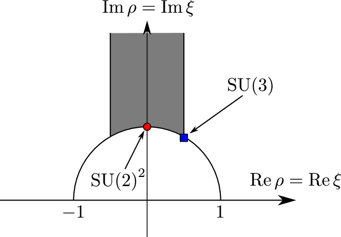
Figure 2: Theory space of the two-component Tomonaga-Luttinger liquid with $\rho=\xi$. The shaded region represents the “fundamental domain”; Because of the duality, different points in the theory space that are related by the duality are isospectral. The fundamental region is a set of representatives for all points related by the duality. I.e., starting from points in the shaded region, by mapping these points by the duality group, the entire theory space is covered. Some spectial points in the theory space are also marked: “SU(3)” represents the SU(3) WZW theory, and “SU(2)²” consists of two copies of SU(2) WZW theories, which may be realized, e.g, as two copies of the XXX spin chain.

When $B_{12}=G_{12}=0$, we have a product of two $c=1$ theories. In this case, the first transformation sends $G\rightarrow G^{-1}$, which corresponds to two independent duality transformations for each $c=1$ theory. Fig. 2 depicts a portion of the space of theories in the $\xi=\rho$ plane together with some points of enhanced symmetry. We anticipate that these theories capture the critical behavior of the gapless degrees of freedom of spin-1 chains such as the model in Eq. (2a).

To deduce the spectrum of these bosonic theories we switch to Euclidean signature $t\rightarrow-it$. We take space-time to be a torus of modulus $\tau=\tau_{1}+i\tau_{2}$ i.e we compactify Euclidean space-time as $x\sim x+2\pi$ and $(x,t)\sim(x,t)+(2\pi\tau_{1},2\pi\tau_{2})$. One can quantize using path integrals, the path integral yields a sum over instanton sectors. We can write in each instanton sector

$$X_{n,w}^{a}=X_{n,w,\,\text{cl}}^{a}+X^{a}_{q}$$ (38)

where

$$X^{a}_{n,w,\,\text{cl}}(x,t)=w^{a}x+\frac{(n^{a}-w^{a}\tau_{1})t}{\tau_{2}}$$ (39)

is a classical solution that winds $n$ and $w$ times along the two non trivial cycles on the torus. The partition function is

$$Z=\sum_{n,w}e^{-S^{cl}_{n,w}}\int[DX_{q}]e^{-S[X_{q}]},$$ (40)

where $S^{cl}_{n,w}$ is the classical action evaluated on shell for Eq. (39), and the quantum path integral is over a continuous uncompactified variable $X_{q}$. The second term in Eq. (32) is a total derivative for periodic functions $X_{q}$ and can be neglected. Thus the integral over $X_{q}$ yields the determinant of the quadratic differential operator appearing in Eq. (32) which is just the Laplacian in the spacetime index times the $G$ matrix in the internal index $a$. After applying a Poisson resummation in $n$ for the classical contribution one finds

$$Z=\frac{1}{\text{det}G^{1/2}}\left(\frac{\tau_{2}}{\det^{\prime}\nabla^{2}}\right)^{c/2}\sum_{p_{L},p_{R}}e^{2\pi i\tau_{1}\left(p\circ p\right)-2\pi\tau_{2}\left(p\cdot p\right)},$$ (41)

where $c=2$,

$$p\circ p =p_{L}^{T}Gp_{L}-p_{R}^{T}Gp_{R},$$

$$p\cdot p =p_{L}^{T}Gp_{L}+p_{R}^{T}Gp_{R},$$ (42)

and

$$p_{L} =\frac{1}{2}\left(G^{-1}(n-Bw)+w\right),$$

$$p_{R} =\frac{1}{2}\left(G^{-1}(n-Bw)-w\right).$$ (43)

The Laplacian determinant can be regularized as $\det^{\prime}\nabla^{2}=\tau_{2}|\eta(\tau)|^{-4}$, where the prime superscript indicates that the zero modes have been removed and $\eta(\tau)$ is the Dedekind eta function.

Comparing with the standard formula for a CFT partition function on the torus one can read off the spectrum of scaling dimensions

$$\Delta=p_{L}^{T}Gp_{L}+p_{R}^{T}Gp_{R}+\sum_{n_{L}>0}n_{L}N^{L}_{n}+\sum_{n_{R}>0}n_{R}N^{R}_{n},$$ (44)

where the last two terms correspond to the determinant of the Laplacian and represent, in canonical quantization, harmonic oscillators indexed by positive integers $n_{L,R}$. $N^{L,R}_{n}$ is the occupation number of oscillator $n_{L,R}$.

For the $\mathrm{SU(3)}_{1}$ WZW theory, we take $G$ and $B$ to be,

$$G=\frac{1}{2}\begin{bmatrix}2&{1}\\ {1}&2\end{bmatrix},\quad B=\frac{1}{2}\begin{bmatrix}0&{1}\\ {-1}&0\end{bmatrix}.$$ (45)

Here $G$ is proportional to the inverse of the Cartan matrix of $\mathrm{SU(3)}$. The above choice of parameters at the $\mathrm{SU(3)}$ point is consistent with that used in the numerical sections below. The relationship to the fields used in the previous section (note they were tilded) is simply a change of basis that diagonalizes $G$ and rescales the diagonal elements to $1$ i.e

$$\phi_{1}=\frac{1}{\sqrt{8\pi}}(X_{1}-X_{2}),\quad\phi_{2}=\sqrt{\frac{3}{8\pi}}(X_{1}+X_{2}).$$ (46)

Since the terms in Eq. (II.3) correspond to the $G$ term in the Hamiltonian (33) we deduce that the continuum version of the transformation ${H}_{\mathrm{SU(3)}}\rightarrow{H}_{\mathrm{SU(3)}}+q_{x}Q_{x}$ is

$$G_{SU(3)}\rightarrow G_{SU(3)}+q_{x}\frac{3}{2}G_{SU(3)}.$$ (47)

This prediction will be tested with the help of accurate numerical calculations, discussed at length in the next section. Fig. 3 depicts the portion of the space that we traverse starting with our choice of parameters for the $\mathrm{SU(3)}$ model and varying $G$ as a function of $q_{x}$. The form of the $G$ matrix in Eq. (47) is consistent with and expected from the $\mathbb{Z}_{3}$ symmetry, i.e., the conservation of $\tilde{N}_{1}-\tilde{N}_{0}$ and $\tilde{N}_{2}-\tilde{N}_{0}$ – see Sec. II.1. The $\mathbb{Z}_{3}$ symmetry can be thought of as a $\frac{2\pi}{3}$ rotation in the root space of $\mathrm{SU(3)}$. In the effective field theory this is represented by the transformation on the currents $(J^{\boldsymbol{\alpha}_{1}},J^{\boldsymbol{\alpha}_{2}},J^{\boldsymbol{\alpha}_{2}})$ (with superscripts defined in Eq. (II.3) ) as $(J^{\boldsymbol{\alpha}_{1}},J^{\boldsymbol{\alpha}_{2}},J^{\boldsymbol{\alpha}_{3}})\to(J^{-\boldsymbol{\alpha}_{2}},J^{\boldsymbol{\alpha}_{3}},J^{-\boldsymbol{\alpha}_{1}})$. In terms of the boson fields $\phi_{1}$ and $\phi_{2}$ which live on the $\mathrm{SU(3)}$ root lattice, this amounts to

$$\boldsymbol{\phi}\to M\cdot\boldsymbol{\phi},\quad M=\left(\begin{array}[]{cc}-1/2&\sqrt{3}/2\\ -\sqrt{3}/2&-1/2\end{array}\right).$$ (50)

In the $\boldsymbol{X}$ basis the $\mathbb{Z}_{3}$ symmetry is represented by

$$\boldsymbol{X}\to M^{\prime}\cdot\boldsymbol{X},\quad M^{\prime}=\left(\begin{array}[]{cc}0&1\\ -1&-1\end{array}\right).$$ (53)

The $G$ matrix in Eq. (47) is left invariant under the $\mathbb{Z}_{3}$ transformation. i.e. we have $M^{\prime T}GM^{\prime}=G$. One can show generally that any symmetric matrix left invariant by $M^{\prime}$ is proportional to $G_{SU(3)}$.

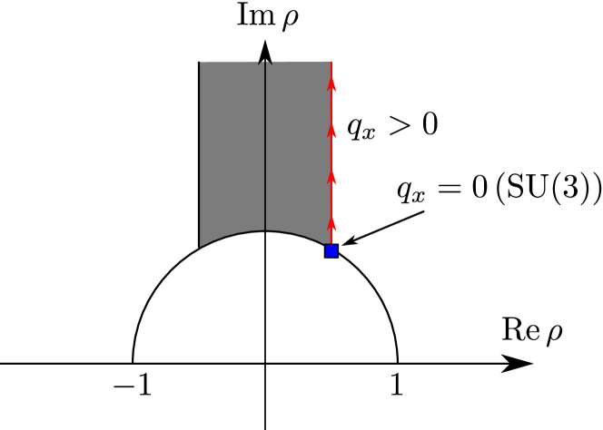
Figure 3: Theory space of the two-component Tomonaga-Luttinger liquid with $\xi=1/2+\sqrt{3}/2i$. The point “$q_{x}=0(\mathrm{SU}(3))$” corresponds to the SU(3) symmetric Lai-Sutherland model. The red line with arrows represents the points in theory space traversed as $q_{x}$ is increased from 0. (The arrows here do not indicate the renormalization group flow.)

III Numerical results establishing correspondence of spin chains to conformal field theory

Having described the field theory for $c=2$ spin chains, we now provide numerical evidence for the proposed correspondence. Our results first focus on various ways of calculating scaling dimensions (44), after which we discuss the procedure for extraction of the TLL parameters $G_{ab}$ and $B_{ab}$ for $a,b=1,2$. We numerically confirm an important prediction of the field theory, namely Eq. (47).

We carried out ED and DMRG calculations for periodic chains; finite size scaling of the energy gaps provides estimates of the lowest scaling dimensions. For bigger open chains, we calculate the same information from the mutual information for spatially disjoint blocks. The mutual information measure is completely determined from the ground state wavefunction, making it useful for situations where obtaining excited states is difficult.

The numerical calculations in this section were performed with a combination of our own codes and the Algorithms and Libraries for Physics Simulations libraries ALPS .

III.1 Inferences from Exact Diagonalization and Density Matrix Renormalization Group

For a 1D periodic chain of length $L$, the scaling dimensions $x_{j}$, corresponding to the $j^{th}$ excited state with energy $E_{j}$, are given by,

$$E_{j}-E_{0}=\frac{2\pi vx_{j}}{L}+\frac{a}{L\log L}$$ (54)

where $a$ is a model specific constant, $v$ is the TLL velocity obtained from the finite size scaling of the ground state energy $E_{0}$,

$$\frac{E_{0}}{L}=e_{\infty}-\frac{\pi cv}{6L^{2}}+\frac{b}{L^{2}(\log L)^{3}}$$ (55)

where $e_{\infty}$ is the energy per site in the thermodynamic limit and $c$ is the central charge and $b$ is a constant. The form of the finite size corrections was derived by Itoi and Kato Itoi_Kato for the $\mathbb{SU}(3)$ symmetric point (i.e. $q_{x}=0)$; here we have assumed the same form holds for $q_{x}>0$.

We note that the above formulas assume all excitations propagate with the same velocity $v$, while for multi-component TLLs, more than one velocity may appear in general. (For more generic models, these formulae need modifications; for example see the work of Ref. Itoi_Affleck on a $\mathrm{SU(2)}\times\mathrm{SU(2)}$ model.) In our model, a naive continuum limit and the bosonization analysis, (20) and (II.3), suggests that the excitations of the system, even when $q_{x}\neq 0$, should be described by a single velocity. We will take this as our working hypothesis. While our spectral analysis by ED/DMRG depends on this assumption, our later analyses based on the entanglement entropy and the mutual information do not.

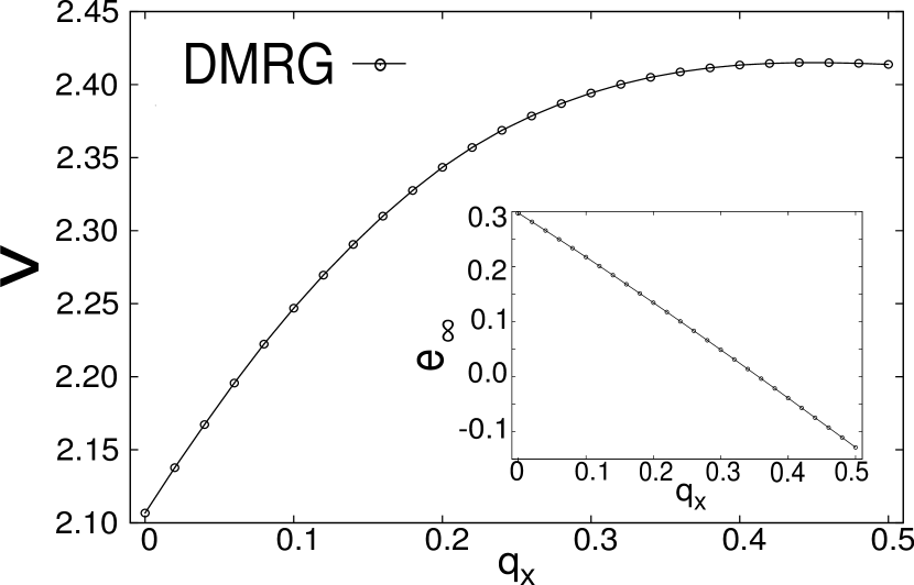
Figure 4: Velocity of the coupled TLLs as a function of $q_{x}$. The inset shows the energy per unit length in the thermodynamic limit as a function of $q_{x}$. The lines are guides to the eye.

Figure 4 shows the TLL velocity $v$ and ground state energy per site in the thermodynamic limit $e_{\infty}$ as a function of $q_{x}$ obtained by fitting our data to Eq. (55). Our results for the $\mathrm{SU(3)}$ symmetric point are in excellent agreement with analytic results Fath and previous numerical studies Fath ; Rachel_SU3 ; Aguado_SU3 ; Lauchli_Schmid_SU3 ; for example, we get $e_{\infty}=0.29679$ and $v=2.107(1)$ which are close to the exact results of $2-\ln 3-\frac{\pi}{3\sqrt{3}}$ and $2\pi/3$ respectively. Care must be taken in comparing our results with studies which parameterize the bilinear and biquadratic terms in the Hamiltonian 2a to be $J\cos\theta$ and $J\sin\theta$ with $\theta=\frac{\pi}{4}$, thus requiring an additional factor of $1/\sqrt{2}$. We have used the value of the central charge $c=2$, which we established independently from the scaling of the entanglement entropy (EE), discussed next.

Before we proceed, we mention an important subtlety associated with the choice of system sizes used in finite-size scaling. In a previous DMRG study on the $\mathrm{SU(3)}$ symmetric model, Ref. Aguado_SU3 showed the absence of the singlet ground state (scaling dimension 0 in the CFT) for chains with lengths $6M+2$ and $6M+4$, where $M$ is a positive integer.  Thus, we restrict ourselves to analyzing chains with lengths that are multiples of 6.

Central charge

We establish the relevant region in parameter space where the TLL physics is expected to hold. For this purpose, we extract the central charge $c$, obtained from the scaling of the EE of a subsystem or "block", readily available in DMRG, as a function of its size $l$. For open chains, the analytic form for the EE, denoted by $S(l)$, is,

$$S(l)=\frac{c}{6}\log\Big{(}\frac{L}{\pi}\sin\Big{(}\frac{\pi l}{L}\Big{)}\Big{)}+S_{0},$$ (56)

where $S_{0}$ is a subleading correction. In Fig. 5 we show the profile of the EE and verify that the $c=2$ fit to it is accurate for all $q_{x}>0$.  However, the EE profile has local structure occurring on the scale of three sites, that arise due to open boundaries. These are not captured by the leading term in Eq. (56). Other similar quality fits are possible with a lower value of $c$; we estimate $c=1.96\pm 0.05$. Also note that $S_{0}$ is non-universal; in this case dependent on $q_{x}$ alone. This explains why the various curves in Fig. 5 differ despite having the same central charge.

Figure 5: Entanglement entropy as a function of block size $(l)$ and its fit to the formula (56) for $c=2$ for a 150 site open chain for various $q_{x}$.

We pursue an understanding of the TLL behavior for all $q_{x}>0$ by considering the case $q_{x}\rightarrow\infty$ Qin_torus . In this limit, the model is a purely classical one, with a macroscopically large number of ground states. To see this, we write out the $Q_{x}$ term on a bond $\langle i,j\rangle$ in terms of $S_{z}$ and $S_{z}^{2}$ operators,

$$U_{x}^{\dagger i}U^{j}_{x}+\text{h.c.}=2-3{S^{i}_{z}}^{2}-3{S^{j}_{z}}^{2}+\frac{9}{2}{S^{i}_{z}}^{2}{S^{j}_{z}}^{2}+\frac{3}{2}S^{i}_{z}S^{j}_{z}.$$ (57)

This expression indicates that the configurations $|\mp 1\pm 1\rangle$ and the configurations $|\pm 1\;0\rangle$ (and $|0\;\pm 1\rangle$) are exactly degenerate and have the lowest energies possible. This means that starting from a spin-1 "Néel" state, for example $|+1-1+1-1\rangle$, one can locally replace each $|+1-1\rangle$ "dimer" by a $|+1\;0\rangle$ without changing the total energy. Thus, there is an exponentially large number of degenerate states. Adding the $\mathrm{SU(3)}$ symmetric term lifts this degeneracy, but the model stays critical. Such a macroscopic degeneracy does not exist in the spin-1/2 XXZ model in the Ising limit; this is why there is a finite value of anisotropy at which the spin-1/2 XXZ model ceases to be critical.

Scaling dimensions and degeneracies

In order to obtain multiple excited states in the same symmetry sector (here sectors of definite $S_{z}$), we perform a state averaging procedure with two target states in the finite system DMRG method. A sequence of bond dimensions varying from $m=400$ to $m=2000$ states and periodic chains of lengths varying from 24 to 66 sites, were studied. For the ED calculations (from 6 to 18 sites), multiple excited states were calculated to give us a picture of the low energy degeneracy structure of this model.

A note about boundary conditions is now in order. Working with open boundary conditions, favorable for DMRG, can complicate the mapping of a spin chain to a conformal field theory: the notion of strict "conformal invariance" is broken. Hence we do not rely on open boundary conditions to give us a picture of the degeneracy structure of this system. That said, scaling dimensions can still be reliably numerically estimated from open chains.

For the $\mathrm{SU(3)}$ symmetric model, it is analytically known that the first excited state is $18$-fold degenerate in the "conformal limit" and the second excited state is $16$-fold degenerate. However, in finite size simulations, the conformal limit is reached rather slowly as a function of system size; more specifically the lattice model (14) flows into the $\mathrm{SU(3)}_{1}$ WZW critical point only logarithmically fast. Thus, we rely only on trends seen in the ED results.

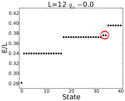
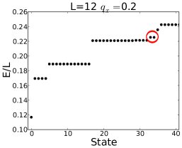
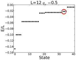
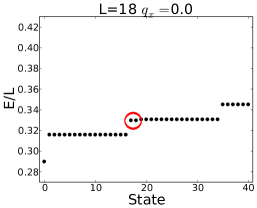
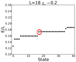
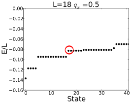
Figure 6: Low energy manifold of the Hamiltonian (2a) for $L=12$ (upper panels) and $L=18$ site periodic chains (lower panels) for different values of $q_{x}$. For $q_{x}=0$, shown in panels (a),(d) the first excited state is known to be $18$-fold degenerate in the conformal limit. On increasing $L$, the inferred trend is that the two higher lying singlets (marked by red circles) descend to possibly join the $16$-fold exactly degenerate states. (b),(e) and (c),(f) show similar trends for $q_{x}=0.2$ and $q_{x}=0.5$; in these cases the degeneracy structure in the conformal limit is narrowed down to a few possibilities.

For the $12$ site ED results, we observe that the low energy manifold consists of a non-degenerate singlet state, two sets of $16$-fold degenerate states [the occurrence of 16 being a consequence of $\mathrm{SU(3)}$ symmetry], followed by two degenerate singlets. As can be seen in Fig. 6(a),(d) on going from $12$ to $18$ sites, the two singlets descend below the second manifold of $16$ states: it is thus conceivable (though not rigorous), that these two states will join the $16$-fold degenerate first excited states resulting in a $18$-fold degeneracy in the conformal limit.

Figure 7: Finite size scaling of the second excited state energy gap for various $q_{x}$. Two independent DMRG calculations are performed, one each for the ground state in the $S_{z}=0$ and $S_{z}=1$ sectors. The fits to Eq. (54), along with the knowledge of the TLL velocity give the second lowest scaling dimension.

Next, consider the effect of adding the $Q_{x}$ term with $q_{x}>0$. From ED, we find that the (exact) $16$-fold degeneracy of the first excited state splits; the first excited state is now $4$-fold degenerate, all corresponding to $S_{z}=0$ states, and the next excited state is $12$-fold degenerate, corresponding to four sets of $S_{z}=\pm 1$ and two sets of $S_{z}=\pm 2$ states. Here too, the two degenerate singlets in the low energy spectrum descend to lower values on increasing the length of the chain, as can be seen in Fig. 6(b),(e) and (c),(f). Based on our experience with the $\mathrm{SU(3)}$ point, we conjecture that restoration of conformal symmetry will result in the $4$-fold degeneracy being transformed to a $6$-fold degeneracy; although other possibilities are not completely ruled out based on this data alone. We expect this degeneracy structure to hold on varying $q_{x}$ only as long as the second excited state does not become the third excited state.

The field theoretic prediction (47) confirms these inferences. Once the second scaling dimension exceeds the value of 1, which occurs around $q_{x}\approx 0.5$, there is a reorganization of energy degeneracies. For $q_{x}\lesssim 0.5$, we deduce that the quantum numbers $\{n_{1},n_{2},w_{1},w_{2}\}$ [see Eq. II.4] corresponding to the lowest $6$ states are $\{\pm 1,\pm 1,0,0\}$, $\{\pm 1,0,0,0\}$ , $\{0,\pm 1,0,0\}$ and those for the next $12$ states are $\{\mp 1,\mp 1,\pm 1,\mp 1\}$, $\{\pm 1,0,0,\pm 1\}$ , $\{0,0,\pm 1,0\}$, $\{0,0,0,\pm 1\}$, $\{0,\pm 1,\mp 1,0\}$ , $\{0,0,\pm 1,\mp 1\}$.

Figure 7 shows fits to Eq. (54), after taking logarithms of both sides, to extract the second scaling dimension $x_{2}$, for various $q_{x}$; similar trends are seen for the first scaling dimension as well. The corrections to scaling are found to increase on going from the $q_{x}=0.0$ to $q_{x}=0.5$. Whether these effects are genuine deviations from the TLL physics or a lack of sufficient size to see "true scaling" can not be definitively established within our present methodology. We believe the deviations close to $q_{x}\approx 0.5$ are due to "energy crossings" (i.e. changing multiplet structure), causing additional level repulsions. Thus, one may need very large sizes to get precise estimates in this region.

Despite this source of inaccuracy, the scaling dimensions vary within 10% when they are computed using Eq. (54) for fixed $L$, over the range of lengths considered ($24-66$ sites). The obtained values validate the correspondence between the lattice model and the CFT and the general trends of their variations with $q_{x}$ support our main conclusions.

III.2 Extracting the lowest scaling dimensions from mutual information

It is difficult to target multiple excited states in DMRG for long chains, especially for a critical system where the entanglement entropy grows logarithmically with system size. Thus it is extremely desirable to have a method to obtain scaling dimensions that involves only the ground state.

Typically this is achieved by measuring ground state correlation functions between two distant regions. However, in the most general setting, we a priori do not know the scaling operators on the lattice i.e. the operators whose expectations are to be measured. To obtain generalized correlation functions between two regions (say $A$ and $B$) we calculate their combined reduced density matrix, for varying separations, and extract the "mutual information" denoted by $I_{AB}$ and formally defined as,

$$I_{AB}\equiv S_{A}+S_{B}-S_{AUB},$$ (58)

where $S_{A}$,$S_{B}$, $S_{AUB}$ is the EE of regions $A$, $B$ and the union of $A$ and $B$ respectively. A schematic of the geometry used for this computation is shown in Fig. 8.

Figure 8: (Color online): (a) Geometry used to compute the mutual information consists of two 2-site blocks separated by distance $r$. The calculations were performed for a 150-site chain with $r<30$, larger $r$ data was discarded to avoid edge effects. Panel (b) shows $F^{2}(x)-1$, derived from the mutual information measure Eq. (58) as a function of the conformal ratio $x$ (see Eq. (62)) calculated with DMRG. It was fitted to the analytic form, Eq. (66) to obtain the lowest scaling dimension.

The mutual information, unlike the block entanglement entropy, is not directly available in DMRG and must be calculated in a matrix product state (MPS) framework. (Practically, this is achieved by reshaping all left and right optimized transformation matrices at the end of the DMRG calculation to get the MPS. Then, the reduced density matrix of disjoint regions is calculated using a partial-contraction scheme discussed in Ref. Muender . More details of our calculations will be provided elsewhere.) The mutual information can also be calculated with Monte Carlo methods in sign-problem free systems Melko_mutual ; Wang_Troyer .

We now discuss extraction of the lowest scaling dimension from $I_{AB}$, for which we briefly present known results from the literature. To do so, we closely follow Ref. Furukawa2009 , whose notations we also use here.

For a CFT, Calabrese and Cardy (CC) Calabrese_Cardy argued that the entanglement entropy of two intervals $A=[x_{1},x_{2}]$ and $B=[x_{3},x_{4}]$ in an infinite lattice is given by,

$$S_{AUB}=\frac{c}{3}\log\left(\frac{x_{21}x_{32}x_{43}x_{41}}{x_{31}x_{42}}\right)+2s_{1},$$ (59)

where $x_{ij}\equiv x_{i}-x_{j}$. The constant $2s_{1}$ is determined by demanding that $S_{AUB}\rightarrow S_{A}+S_{B}$ in the limit $x_{21},x_{43}<<x_{31},x_{42}$. Rewriting this formula in terms of the mutual information (i.e. on subtracting out the single interval contributions), one gets,

$$I_{AB}^{CC}=\frac{c}{3}\log\left(\frac{x_{32}x_{41}}{x_{31}x_{42}}\right).$$ (60)

For a finite periodic chain, one replaces $x_{ij}$ by the cord distance $L/\pi\sin(\pi x_{ij}/L)$, this results in,

$$I_{AB}^{CC}=\frac{c}{3}\log\left(\frac{\sin(\pi x_{32}/L)\sin(\pi x_{41}/L)}{\sin(\pi x_{31}/L)\sin(\pi x_{42}/L)}\right).$$ (61)

It is thus convenient to define the conformal ratio $x$ as,

$$x\equiv\frac{\sin(\pi x_{32}/L)\sin(\pi x_{41}/L)}{\sin(\pi x_{31}/L)\sin(\pi x_{42}/L)}.$$ (62)

The notion of mutual information can be generalized beyond the von-Neumann entropy, which is assigned an index $n=1$, and thus denoted more generally by $I^{(n)}_{AB}$. This is achieved by the following replacements in the CC formulae,

$$S_{1}\rightarrow S_{n},\quad c\rightarrow\frac{1+n}{6n}c.$$ (63)

Ref. Furukawa2009 found that the true mutual information and the CC mutual information differ by a function $f^{n}(x)$,

$$I^{(n)}_{AB}-{I^{(n)}}^{CC}_{AB}=f^{(n)}(x),$$ (64)

which is reparameterized as,

$$\frac{1}{n-1}F^{(n)}(x)\equiv f^{(n)}(x).$$ (65)

Calabrese and co-workers CCTonni ; Alba_Calabrese have shown that for $n>1$ and in the limit of small $x$,

$$F^{(n)}(x)-1 =\left(\frac{x}{4n^{2}}\right)^{\alpha}s_{2}(n)+\left(\frac{x}{4n^{2}}\right)^{2\alpha}s_{4}(n)$$

$$\quad+(\text{higher order}),$$ (66)

where $\alpha$ is twice the lowest scaling dimension $x_{1}$. The coefficients $s_{2}(n)$ and $s_{4}(n)$ are the contributions in the small $x$ expansion coming from the two and four-point functions of the operator in the CFT with the lowest scaling dimension.

Two concerns when using equation (66) in numerical simulations are (1) it holds only for an infinite lattice and (2) it assumes that the non-zero contributions are solely from the operator with the lowest scaling dimension. However, for a finite system there are contributions from all operators. Thus the lowest scaling dimension fitted is simply an effective one trying to mimic the action of a linear combination of many (different scaling) operators. Empirically, for an open chain of 150 sites, all the errors (systematic and due to fitting) appear to be within 10%, which is roughly the error we also obtain from fitting to energies.

Our results for fits to a power law for $F^{2}(x)-1$ for various $q_{x}$ are shown in Fig. 8. The overall fits are reasonable, though there are local features not captured by Eq. (66): just like the case of the EE, these are attributed to open boundaries. Such features are also seen in the spin-1/2 XXZ model, studied independently by Ref. Barcza .

Figure 9: The main panel shows the first two scaling dimensions, $x_{1}$ and $x_{2}$, as a function of $q_{x}$, obtained from finite size scaling of energy gaps obtained from a combination of exact diagonalization (ED) and the density matrix renormalization group (DMRG) for periodic chains denoted by PBC. The $c=2$ conformal field theory (CFT) prediction is also shown. The inset shows the lowest scaling dimension obtained from the mutual information (MI) measure (see text), computed within the DMRG/Matrix product state framework for an open chain of 150 sites.

III.3 Extraction of TLL parameters

Fig. 9 shows the lowest two scaling dimensions obtained from finite size scaling of energy gaps as a function of $q_{x}$. The inset shows the lowest scaling dimension from the mutual information method; with this metric, we were able to explore a larger range of $q_{x}$. The general agreement (within errors) between these independent metrics confirms our that we can reliably calculate lowest scaling dimensions. Thus we proceed to discuss the extraction method for the four TLL parameters.

Given a trial set of $G_{ab}$ and $B_{ab}$, we calculate the lowest 18 scaling dimensions, which need not be distinct, and denote them by $x_{i}^{\text{G,B}}$. We then evaluate a cost function,

$$C\text{(G,B)}\equiv\sum_{i}(x_{i}^{\text{G,B}}-x_{i}^{\text{DMRG}})^{2}$$ (67)

and minimize it with respect to $G_{11},G_{12},G_{22}$ and $B_{12}$ to obtain the best fit. We used the Nelder-Mead simplex algorithm built into the GNU Scientific library for this purpose.

In order to confirm our inferences about the nature of the degeneracies in the low energy manifold, we attempted to fit to two degeneracy structures for the first and second excited states. First, we assumed that the degeneracy (denoted by $g_{i}$) of the first two distinct scaling dimensions to be $(g_{1},g_{2})=(6,12)$ and in the second case $(g_{1},g_{2})=(4,12)$. In all cases, for $q_{x}<0.5$, we found the former gave a significantly better fit to the CFT formulae (44). In fact, attempts to use the $(4,12)$ structure gave optimized solutions closer to a $(g_{1},g_{2},g_{3})=(4,2,12)$ degeneracy structure, hinting that the imposed structure was incorrect. The quality of our fits are checked by how well the scaling dimensions were reproduced; for the correct degeneracy structure, these agreed to within $\pm 0.03$.

The agreement of the values of the measured and expected scaling dimensions, shown in Fig. 9, strongly indicates an internally consistent scenario for the lattice model to CFT mapping. This is also equivalently seen in the extracted TLL parameters, shown in Fig. 10, which are consistent with Eq. (47): they satisfy the expected relation $G_{11}=G_{22}=2G_{12}$. The relative error in the scaling dimensions propagates to these parameters; for example, the overall error in $G_{11}$ is roughly twice the error in $x_{2}$. As expected from the duality explained in section II.4, the scaling dimensions depend on $B_{12}$ up to an integer shift. Thus we focus on a particular representation and find that $B_{12}=1/2$ explains our data for all $q_{x}$. Finally, even though we have shown data only for $q_{x}<0.5$, the mutual information data in Fig. 9 (inset) suggests the validity of the theory for larger $q_{x}$.

Figure 10: TLL parameters as a function of $q_{x}$ extracted from matching scaling dimensions to a $c=2$ CFT. The main panel shows $G_{11}$ as a function of $q_{x}$ and we find $G_{11}=G_{22}=2G_{12}$. The inset shows $B_{12}$ which is found to be constant. The CFT prediction is shown by the solid lines.

IV Conclusion

In conclusion, we have developed an analytic correspondence between $c=2$ free boson theories and microscopic spin-1 models, using bosonization techniques. For the particular form of Hamiltonian considered (Eq. (2a)), we made a prediction for the value of the Tomonaga-Luttinger liquid (TLL) parameters as a function of $q_{x}$, the parameter characterizing the lattice model.

To build evidence on the numerical front, we performed exact diagonalization (ED) and density matrix renormalization group (DMRG) calculations to obtain the lowest scaling dimensions from the energetics of the system; a scheme feasible for short periodic chains. However, our use of the mutual information entropy between disjoint blocks, calculated solely from the ground state, provides a promising route to extend these calculations for long chains.

Using this numerical data and the mapping from spin-chains to $c=2$ theories, we deduced the value of all four TLL parameters as a function of $q_{x}$. We expect our analyses to apply to more general situations, for eg. the model in Eq. (2a) with non zero $q_{y}$. In future work, we aim to extend these ideas to calculate multiple low-lying scaling operators and dimensions of the $c=2$ CFT using the correlation density matrix Cheong_Henley ; Muender .

Our broader objective is an effort to develop generic methods to map lattice models to multi-component field theories. We anticipate that this multi-scale modelling approach will be useful for understanding the physics at very large length scales; sizes that may not be directly accessible in numerical simulations. Once we have built confidence in the mapping between the lattice and continuum descriptions, we can use the (often known) predictions of the latter.

V Acknowledgements

We thank Christopher Henley, Dunghai Lee, Eduardo Fradkin, Shunsuke Furukawa, Garnet Chan, Andreas Läuchli, Victor Chua and Norman Tubman for discussions. This work has been supported by SciDAC grant DE-FG02-12ER46875. Computer time was provided by XSEDE and the Taub campus cluster at the University of Illinois Urbana-Champaign/NCSA. SR is supported by the A. P. Sloan Foundation.

References

- (1) P. Calabrese and J. Cardy, Journal of Statistical Mechanics: Theory and Experiment 2004, P06002 (2004).
- (2) H. Li and F. D. M. Haldane, Phys. Rev. Lett. 101, 010504 (2008).
- (3) S. Ryu and T. Takayanagi, Phys. Rev. Lett. 96, 181602 (2006).
- (4) M. Headrick, Phys. Rev. D 82, 126010 (2010).
- (5) J. McMinis and N. Tubman, Phys. Rev. B 87, 081108 (2013).
- (6) M. Hastings, I. González, A. Kallin, and R. Melko, Phys. Rev. Lett. 104, 157201 (2010).
- (7) S. Ryu and Y. Hatsugai, Phys. Rev. B 73, 245115 (2006).
- (8) R. Thomale, D. P. Arovas, and B. A. Bernevig, Phys. Rev. Lett. 105, 116805 (2010).
- (9) R. Lundgren et al., Phys. Rev. Lett. 113, 256404 (2014).
- (10) S.-A. Cheong and C. Henley, Phys. Rev. B 79, 212402 (2009).
- (11) W. Muender et al., New Journal of Physics 12, 075027 (2010).
- (12) C. L. Henley and H. J. Changlani, Journal of Statistical Mechanics: Theory and Experiment 2014, P11002 (2014).
- (13) R. Melko, A. Kallin, and M. Hastings, Phys. Rev. B 82, 100409 (2010).
- (14) G. Barcza, R. M. Noack, J. Solyom, O. Legeza, arXiv:1406.6643 (unpublished).
- (15) S. Furukawa, V. Pasquier, and J. Shiraishi, Phys. Rev. Lett. 102, 170602 (2009).
- (16) S.-i. Tomonaga, Progress of Theoretical Physics 5, 544 (1950).
- (17) J. M. Luttinger, Journal of Mathematical Physics 4, (1963).
- (18) T. Giamarchi, Quantum Physics in One Dimension, Volume 121 of International Series of Monographs on Physics, Clarendon Press, (2003).
- (19) F. D. M. Haldane, Journal of Physics C: Solid State Physics 14, 2585 (1981).
- (20) M. Bockrath, D. H. Cobden, J. Lu, A. G. Rinzler, R. E. Smalley, L. Balents and P. L. McEuen, Nature 397, 598-601 (1999).
- (21) H. Ishii, H. Kataura, H. Shiozawa, H. Yoshioka, H. Otsubo, Y. Takayama, T. Miyahara, S. Suzuki, Y. Achiba, M. Nakatake, T. Narimura, M. Higashiguchi, K. Shimada, H. Namatame, M. Taniguchi, Nature 426, 540-544 (2003).
- (22) A. Yacoby et al., Phys. Rev. Lett. 77, 4612 (1996).
- (23) S. R. White, Phys. Rev. Lett. 69, 2863 (1992).
- (24) A.M. Läuchli,arxiv:1303.0741 (unpublished).
- (25) E. Jeckelmann, Journal of Physics: Condensed Matter 25, 014002 (2013).
- (26) C. Karrasch and J. Moore, Phys. Rev. B 86, 155156 (2012).
- (27) M. Dalmonte, E. Ercolessi, and L. Taddia, Phys. Rev. B 85, 165112 (2012).
- (28) R. Lundgren, Y. Fuji, S. Furukawa, and M. Oshikawa, Phys. Rev. B 88, 245137 (2013).
- (29) T. Sakai et al., Journal of Physics: Condensed Matter 22, 403201 (2010).
- (30) H. J. Schulz, Phys. Rev. B 53, R2959 (1996).
- (31) H.J. Schulz, “Correlated Fermions and Transport in Mesoscopic Systems”, ed. T. Martin, G. Montambaux, J. Tran Thanh Van (Editions Frontieres, Gif–sur–Yvette, 1996), p. 81.
- (32) J. Schnack et al., Phys. Rev. B 70, 174420 (2004).
- (33) H. Manaka et al., Journal of the Physical Society of Japan 78, 093701 (2009).
- (34) R. V. Mishmash et al., Phys. Rev. B 84, 245127 (2011).
- (35) R. Chen et al., Phys. Rev. B 87, 165123 (2013).
- (36) M. Sato, Phys. Rev. B 75, 174407 (2007).
- (37) M. P. Qin et al., Phys. Rev. B 86, 134430 (2012).
- (38) C. K. Lai, Journal of Mathematical Physics 15, (1974).
- (39) B. Sutherland, Phys. Rev. B 12, 3795 (1975).
- (40) C. Itoi and M.-H. Kato, Phys. Rev. B 55, 8295 (1997).
- (41) N. Papanicolaou, Nuclear Physics B 305, 367 (1988).
- (42) F. D. M. Haldane, Phys. Rev. Lett. 50, 1153 (1983).
- (43) I. Affleck, T. Kennedy, E. H. Lieb, and H. Tasaki, Phys. Rev. Lett. 59, 799 (1987).
- (44) P. Millet et al., Phys. Rev. Lett. 83, 4176 (1999).
- (45) M. Oshikawa, C. Chamon, and I. Affleck, Journal of Statistical Mechanics: Theory and Experiment 2006, P02008 (2006).
- (46) I. Affleck, in Fields, Strings and Critical Phenomena, 1988 Les Houches Lecture Notes, edited by E. Brezin and J. Zinn-Justin (Elsevier, Amsterdam, 1989), p. 564.
- (47) P. D. Francesco, P. Mathieu, and D. Senechal, Conformal Field Theory, Graduate Texts in Contemporary Physics (Springer, ADDRESS, 1997).
- (48) M. Green, J. Schwarz, and E. Witten, Superstring Theory: Introduction, Cambridge monographs on mathematical physics (Cambridge University Press, ADDRESS, 2012).
- (49) P. Ginsparg, in Fields, Strings and Critical Phenomena: Proceedings (Les Houches 1988), ed. by E. Brezin and Jean Zinn-Justin, pp. 1-168. Amsterdam: North-Holland (1990).
- (50) S. Dulat and K. Wendland, Journal of High Energy Physics 2000, 012 (2000).
- (51) K. Becker, M. Becker, and J. Schwarz, String Theory and M-Theory: A Modern Introduction (Cambridge University Press, ADDRESS, 2006).
- (52) A. Giveon, M. Porrati, and E. Rabinovici, Physics Reports 244, 77 (1994).
- (53) B. Bauer et al., Journal of Statistical Mechanics: Theory and Experiment 2011, P05001 (2011).
- (54) C. Itoi, S. Qin, and I. Affleck, Phys. Rev. B 61, 6747 (2000).
- (55) G. Fáth and J. Sólyom, Phys. Rev. B 51, 3620 (1995).
- (56) M. Führinger et al., Annalen der Physik 17, 922 (2008).
- (57) M. Aguado et al., Phys. Rev. B 79, 012408 (2009).
- (58) A. Läuchli, G. Schmid, and S. Trebst, Phys. Rev. B 74, 144426 (2006).
- (59) This observation can possibly be better understood by extracting the scaling operators from numerics. This involves determining a coarse grained operator that spans three sites; a direction we will not explore in the present paper.
- (60) Practically this was checked for .
- (61) L. Wang and M. Troyer, Phys. Rev. Lett. 113, 110401 (2014).
- (62) P. Calabrese, J. Cardy, and E. Tonni, Journal of Statistical Mechanics: Theory and Experiment 2011, P01021 (2011).
- (63) V. Alba, L. Tagliacozzo, and P. Calabrese, Phys. Rev. B 81, 060411 (2010).