Will solid-state drives accelerate your bioinformatics?
In-depth profiling, performance analysis, and beyond

Sungmin Lee¹, Hyeyoung Min², and Sungroh Yoon¹

¹Electrical and Computer Engineering, Seoul National University, Seoul 151-744, Korea
²College of Pharmacy, Chung-Ang University, Seoul 156-756, Korea

1 Introduction

Enabled by breakthroughs in data generation, collection, and analysis technologies, we are living in the era of big data[1]. Novel data-driven research and business opportunities are envisioned in many disciplines, and biomedicine is not an exception. The recent trend toward personalized precision medicine has triggered the accumulation of a great deal of biomedical data from various sources [2], such as (epi-/meta-/pharmaco-)genomics, transcriptomics, proteomics, metabolomics, wearable mobile devices, and crowd-sourced scientific games[3].

The need for efficient processing of biomedical big data has been partly met by parallel computing that spans from shared-memory machines (e.g., multicore CPUs and GPUs) to distributed systems (e.g., MPI/Hadoop/Spark-based cloud computing). For instance, the Broad Institute and Intel Corporation have been jointly working on parallelizing the Genome Analysis Toolkit (GATK, [4]). Its sequential implementation takes more than 360 hours to genotype a single personal human genome, but this collaboration recently reported that it is possible to gain a more than 10-fold speedup by employing multicore processors.

Nevertheless, the time demand of many bioinformatics programs still remains unsatisfactory for large-scale practical uses, due to various reasons that hinder acceleration by parallelization, such as limited parallelism in the algorithm, frequent data transfers among computing units, and high cost (time and resources) of parallelization. Additional methods for acceleration (other than parallel computing) have been sought, including storage-centric approaches that are emerging with the renewed interest in near-data processing [5].

Traditionally, there has been a substantial difference between the pace of improvements in CPUs and storage technologies, also known as the CPU-IO performance gap [6]. With the advent of NAND flash-based solid-state drives (SSDs), this gap is becoming narrower than ever, along with the gradual transition to fast host interfaces (such as PCI Express). SSDs show substantially higher performance than hard disk drives (HDDs) especially when there are frequent random input-output (IO) requests [7], not to mention their mechanical advantages originating from the lack of moving internal components. In data science and engineering, various workloads with abundant random IOs have been successfully accelerated often by a simple ‘drop-in’ replacement of HDDs by SSDs. Furthermore, traditional data analytics algorithms are being redesigned to fully exploit the new, fast secondary storage [8].

Despite the simplicity (e.g., drop-in replacement without any other modifications) and continuous cost reduction fostering widespread use of SSDs, there has been little review of SSD-based profiling and performance exploration in the bioinformatics community. In this review, we compare the performance of 23 well-known bioinformatics programs (see Table LABEL:t:tool_list) using multiple types of SSDs and HDDs. The programs we analyze cover traditional and emerging bioinformatics areas of high importance, such as sequence alignment, genome assembly, read mapping, gene expression analysis, motif finding, variant calling, and metagenomics. We classify these bioinformatics tools into two groups, depending on the effectiveness of SSDs on speedup, and investigate the factors that cause the difference from a storage system perspective.

Based on the insight obtained from the research, we further discuss issues in implementing and selecting bioinformatics algorithms and pipelines with the SSDs under consideration. For instance, we show that acceleration by parallelization can be accompanied by SSDs to yield extra runtime improvements. Examples include ABySS[9] (a parallel short-read assembler) and the GATK (which uses the MapReduce framework [10]). In our experiments, ABySS and a variant-calling pipeline using the GATK achieved 51.7 and 35.7 times speedup, respectively, when using SSDs. Another discussion on SSD-based acceleration comes from the short-read aligners for next-generation sequencing (NGS) [11]. We compare Maq [12], Burrows-Wheeler Aligner (BWA, [13]), and Bowtie 2 [14] in terms of runtime and quality metrics before and after using SSDs and analyze the result from storage-system perspectives. Based on this analysis, we further discuss how to assess alternative bioinformatics programs in terms of the viability of SSD-based acceleration.

To the best of the authors’ knowledge, this review presents the first in-depth profiling analysis of major bioinformatics programs targeted at revealing opportunities and limitations of using SSDs for acceleration of bioinformatics tools. We hope that this review can provide useful directions and tips that should accompany future bioinformatics algorithm design procedures that properly consider new generations of powerful storage devices.

[ caption = List of the twenty three bioinformatics programs profiled and analyzed in this work, label = t:tool_list, doinside = ]llllll []G₊, programs with 2x or more speedup; G₀, programs with negligible improvements; MSA, multiple sequence alignment; NJ, neighbor joining; HMM, hidden Markov model; EM, expectation maximization; $\dagger$ speedup by Intel 520 SSD over Seagate Barracuda HDD [see Tables LABEL:t:ssd_spec and LABEL:t:hdd_spec for specifications and Table LABEL:t:data_list for input data]. Name Task Main algorithm Source Speedup^†
G₊ GATK BaseRecal Base quality recalibration generates recalibration table based on covariates [4] 78.4
Samtools Utility tool sorting, merging, indexing large sequence alignment [15] 77.2
ABySS NGS assembler distributed de Bruijn graph, hash table searching [9] 51.7
Cluster3 Microarray analsysis calculating pairwise sequence distance, clustering [16] 50.0
Blat Sequence alignment index searching on non-overlapping k-mers [17] 23.6
Reptile NGS denoising MSA with Hamming distance, k-spectrum extraction [18] 13.7
GATK Aligner Sequence realignmentSmith-Waterman local realignment[4] 12.6
Maq NGS assembler ungapped sequence alignment, maximizing posterior probability [12] 10.1
Tophat RNA-seq analysissegmented sequence alignment using Bowtie [19] 3.2
MC-UPGMA Microarray analsysis memory-constrained multi-round hierarchical clustering [20] 2.7
G₀ BWA Sequence alignmentBurrows-Wheeler transform, trie traversal [13] 1.09
Blast Sequence alignmentseed-based local sequence alignment [21] 1.08
ClustalW Sequence alignmentmultiple sequence alignment using NJ guide tree [22] 1.06
GATK Unified Genome variant calling Bayesian likelihood modeling [4] 1.05
GATK PrintReads Utility toolsorting, and merging sequence alignments [4] 1.03
Scripture RNA-seq analysissequence alignment using TopHat, graph traversal [23] 1.02
IGVtools Utility toolsequence alignment indexing, sorting [24] 1.02
Meme Motif findingexpectation-maximization, greedy search [25] 1.00
Bowtie 2 Sequence alignmentBurrows-Wheeler-based sequence alignment [14] 1.00
Mosdi Motif findingHMM-based statistical modeling, suffix tree traversal [26] 1.00
AmpliconNoise NGS denoisingNeedleman-Wunsch, hierarchical clustering, EM [27] 1.00
Weeder Motif findingsuffix tree-based exhaustive searching [28] 1.00
ErmineJ Microarray analsysispermutation, rank-based statistics analysis [29] 0.97

2 Results: SSD-leveraged Acceleration

2.1 SSD-leveraged resurrection of hash-based aligners

As a warm-up case, we tested how using SSDs can accelerate well-known bioinformatics programs simply by the drop-in replacement of HDDs by SSDs in the same computer without any other modifications in hardware or software. To this end, we used the short-read alignment tools for next-generation sequencing [11]. Note that the first wave of such tools, mostly hash-based methods (e.g., Maq), has been gradually replaced by Burrows-Wheeler Transform (BWT) based methods (e.g., Bowtie 2 and BWA), mainly because of their rapid searching capabilities backed by smaller memory footprints, albeit a sacrifice in accuracy [30].

Figure 1 shows the running time and quality of Maq, BWA, and Bowtie 2. Refer to the figure caption for details of the devices and the data set used. As expected, when HDDs are used, the runtime of Maq is significantly higher than that of Bowtie 2 or BWA. Maq is a hash-based method while Bowtie 2 and BWA are more memory-efficient BWT-based techniques. Consequently, these second-generation methods usually run faster than the first-generation aligners especially when the data size is large and swaps frequently occur. When SSDs are used, Maq is still the slowest, but the runtime gap has become dramatically narrower, leveraged by the enhanced IO performance and reduced swap cost of SSDs.

Given this boost in runtime and the advantage in quality measured using various metrics as shown in Figure 1(b), it would be possible to use Maq instead of Bowtie 2 or BWA when high values for quality metrics are desired. A simple drop-in replacement of HDDs by SSDs has made the earlier generation of tools competitive to the later generation of tools to some extent.

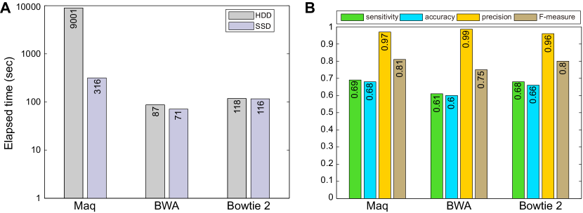
Figure 1: Performance comparison of three short-read aligners: Maq [12], BWA [13], and Bowtie 2 [14]. (a) Runtime. (b) Quality measured in sensitivity, accuracy, precision, and F-measure. [SSD: Samsung 840 Pro (128GB), HDD: Seagate Barracuda (1TB, 7200rpm), data: Staphyloccus aureus whole genome sequence [31]]

2.2 Measuring speedup of bioinformatics programs

To further investigate what kind of bioinformatics tools can be accelerated by using SSDs, we prepared a total of 23 bioinformatics programs listed in Table LABEL:t:tool_list and measured the speedup by drop-in replacements of HDDs by SSDs. Refer to Tables LABEL:t:ssd_spec and LABEL:t:hdd_spec in Section 5.1 for more details of the experiments.

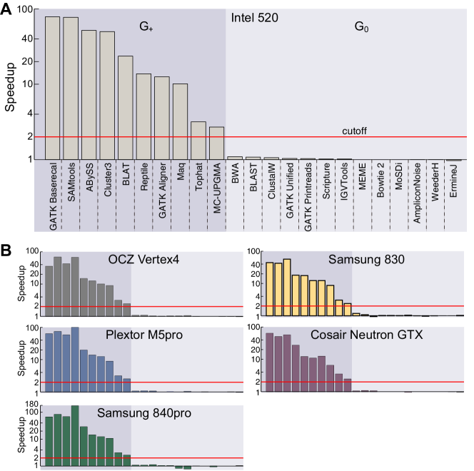
Figure 2: Speedup of 23 bioinformatics programs by drop-in replacements of HDDs by SSDs. [G₊, programs with 2x or more speedup; G₀, programs with negligible improvements] (a) SSD: Intel 520 (120GB), HDD: Seagate Barracuda (1TB, 7200rpm). (b) SSD: five different models listed in Table LABEL:t:ssd_spec, HDD: the same as in (a). The order of the programs placed below the x-axis remains the same as in (a). Additional results form comparing a complete set of SSD-HDD pairs is available at http://best.snu.ac.kr/pub/biossd.

The result is shown in Figure 2. Using SSDs yielded substantial speedup for certain programs (e.g., GATK BaseRecal) but was not always effective. Regardless of the specific SSD used for measurement, we were able to divide the 23 programs into two groups, namely G₊ (the programs with 2x or more speedup) and G₀ (the programs with negligible or no improvements). The programs in each of these two groups are listed in Table LABEL:t:tool_list. To find the root-cause reason that separates these two groups, we will further profile and analyze these 23 programs from storage system perspectives in Section 3.

Note that the result shown in Figure 2(a) is from using a 120GB Intel 520 SSD in place of a 1TB Seagate Barracuda HDD (3.5 inch). The results from the other five SSDs are shown in Figure 2(b). Using different SSDs and HDDs did not change the group membership of each program but only its speedup ranking within each group. In what follows, we thus present the results obtained from using an Intel 520 and a Seagate Barracuda unless otherwise stated. The results from using the other combinations of SSDs and HDDs are available online at http://best.snu.ac.kr/pub/biossd.

2.3 Accelerating bioinformatics pipelines by SSDs

Based on the initial profiling results described in Section 2.2, we further tested if there is any performance gain by using SSDs for running a bioinformatics pipeline that consists of multiple component programs. As shown in Figure 3, we measured the runtime of three bioinformatics pipelines before and after a drop-in replacement of HDDs by SSDs. The pipelines analyzed are for variant calling by the Genome Analysis Toolkit (GATK) [4], whole-genome sequence assembly and annotation [33], and transcriptome reconstruction [23].

Figure 3(a) illustrates the breakdown of the runtime of the GATK pipeline for SNP calling. The pipeline consists of the component tools for sequence alignment and formatting using BWA [13] and Samtools [15], sequence realignment (GATK Aligner), sequence base-quality recalibration (GATK BaseRecal), result merge (GATK PrintReads), and SNP and indel calling (GATK Unified). By a simple drop-in replacement, we could achieve more than a 35 times decrease in the runtime of the whole pipeline. The majority of the speedup is due to the reduced runtime of formatting (Samtools, 77.2x speedup), sequence realignment (GATK Aligner, 12.6x speedup), and base-quality recalibration (GATK BaseRecal, 78.4x speedup).

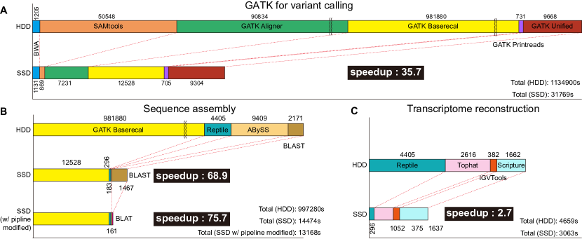
Figure 3: SSD-based acceleration of bioinformatics pipelines. (a) variant calling by GATK [4]. [data: NA12878 human whole genome sequence [32]] (b) Sequence assembly and annotation [33]. [data: Staphyloccus aureus whole genome sequence [31]] (c) Transcriptome reconstruction [23]. [data: Mouse (mm9) reads (see Table LABEL:t:data_list for a link)]

The second pipeline depicted in Figure 3(b) carries out sequence assembly and annotation. The first three steps account for most of the improvements and consist of GATK Baserecal, Reptile [18], and ABySS [9], which are all accelerated significantly by SSDs, according to Table LABEL:t:tool_list. Replacing Blast with Blat gave additional runtime reduction, producing 75.7x total speedup over HDDs. Of note is that ABySS, a parallel short-read assembler, got boosted more than 50 times by SSDs. This is an example in which combination of computing parallelization and SSD-based storage can yield a dramatic performance gain.

Figure 3(c) shows the third pipeline for transcriptome reconstruction [23] in RNA-seq experiments [34]. The amount of speedup was smaller than the above two. Although the most time-consuming step (Reptile) of the pipeline was accelerated significantly by SSDs, the total runtime of the pipeline was relatively shorter, and the effect of runtime reduction in Reptile got eclipsed by the Scripture [23] step. We expect that using a larger data set will reveal the effect of SSD-based runtime reduction. (Related results are presented in Section 3.6.)

3 Results: Profiling and Analysis

This section elaborates how we profiled and analyzed the 23 bioinformatics programs under study. We first measured important storage features for each program and then clustered the programs with respect to the measured feature values. The measurement and clustering allowed us to discover IO patterns that can not only differentiate G₊ and G₀ but also provide useful insight into when SSDs can be effective for acceleration and when not.

3.1 Measuring storage features

For each of the 23 bioinformatics programs, we measured eight features that are widely used in storage research. Table LABEL:t:io_features lists more details of these features and their acronyms to be used in the paper. Using these features, we will consider the randomness and the amount of IOs involved in these 23 programs. The amount of IOs is measured by Butil, Riops, Wiops, and Pfault, whereas the IO randomness is measured by CAR, Rsize, Wsize, and WBlen. More details can be found in Section 5.2.

[ caption = List of storage features used (see Section 5.2 for details), label = t:io_features, pos = t, ]lll ID Feature When high (low)
Butil interface bandwidth utilization large (small) data transfers
Riops read IO per second (in)frequent reads
Wiops write IO per second (in)frequent writes
Pfault # page faults per second (in)frequent page swaps
CAR Consecutive Access Ratio sequential (random) access
Rsize read size per request sequential (random) reads
Wsize write size per request sequential (random) writes
WBlen write buffer length many (few) writes in queue

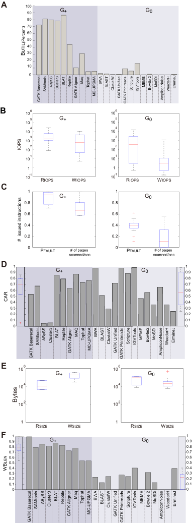
Figure 4: Storage feature measurements. (a) Bandwidth utilization of host-storage interface (Butil). (b) Read IOPS (Riops) and write IOPS (Wiops). (c) The number of page faults per second (Pfault). (d) Consecutive Access Ratio (CAR). (e) Read size per request (Rsize) and write size per request (Wsize). (f) Storage buffer queue length (WBlen). [see Table LABEL:t:io_features and Section 5.2 for more details of these features]

The measurement results are shown in Figure 4. Overall, we can make the following observations:

• The features related to the number of IO operations issued by the host (Riops and Wiops) have higher values for G₊.

• The features related to the amount or frequency of transfers between the host memory and the storage (Butil and Pfault) are higher for G₊.

• Each of the features related to IO randomness (Rsize, Wsize, and CAR) shows a different pattern: Rsize is higher for G₀ (i.e., negligible speedup for programs with many sequential reads), Wsize is higher for G₊ (i.e., notable speedup for programs with many random writes), and CAR is moderately higher for G₊.

• The feature affected by both the amount of data transfers and IO randomness (WBlen) is consistently higher for G₊.

O1 and O2 can be explained by the fact that SSDs normally support higher IOPS while incurring less overheads for swaps. Thus, the programs with more IO operations and page faults can be more effectively accelerated by SSDs. O3 and O4 are related to the fact that SSDs are superior for handling random IOs, but part of these observations is not completely intuitive at first.

For instance, not only SSDs but also HDDs normally have DRAM buffers that can hide latency incurred by random writes, implying that programs with many random writes will not see significant speedup by using SSDs. This implication is seemingly against O3. In addition, according to O3, CAR is higher for G₊, which seems to suggest that the programs in G₊ show less randomness. Given that SSDs are effective for handling random IOs, O3 is seemingly inconsistent with the fact that the programs in G₊ are accelerated more by using SSDs. Section 3.3 include further explanations of O3 and O4 that can answer these riddles.

3.2 Pattern discovery by clustering

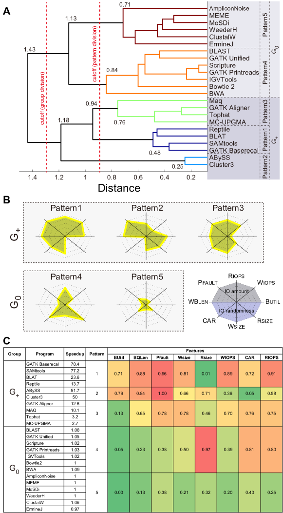
Figure 5: Clustering bioinformatics programs based on the eight storage features listed in Table LABEL:t:io_features. (a) Dendrogram and pattern definitions. The numbers represent the pairwise distance. (b) Radar chart representations of the average feature values for each pattern. Legend is also shown. (c) The numberical values of the average features depicted on the axes of the radar charts in (b). The names and the speedup amounts are also presented.

Observations O1–O4 only reveal overall trends. For a specific program, the prediction of the effectiveness of SSD simply using individual storage features alone may not be accurate. For example, some programs in G₀ have high Butil, Riops, and Wiops but do not show significant speedup. To see the combinations of features leading to effective speedup and to find patterns that can help grouping bioinformatics programs in terms of IO behavior, we tried clustering the 23 programs based on the eight storage features.

Figure 5(a) shows the dendrogram obtained by agglomerative hierarchical clustering with the average linkage. We use the Euclidean distance metric to measure the distance between two vectors, each of which consists of the eight measurement values normalized and ranged in $[0,1]$ (see Section 5.1). Cutting the dendrogram near the root bifurcation point reveals the two groups G₊ and G₀. Cutting it at the smaller distance as shown in the plot produces five clusters or patterns. Group G₊ consists of three patterns (denoted by P1, P2, and P3), while group G₀ contains two (denoted by P4 and P5).

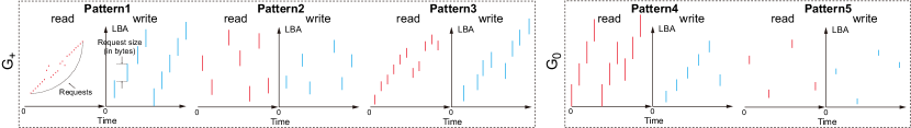
Figure 6: Representative IO traces for each of the five patterns shown in Figure 5. A vertical bar corresponds to an IO request, and its length represents the read or write size. The quantity of vars in each plot is proportional to the IO amount, while the distribution of accessed LBAs represents the IO randomness. [LBA, logical block address; G₊, programs with 2x or more speedup; G₀, programs with negligible or no improvements]

Figure 5(b) shows the radar chart representation of the average feature values for each pattern. Figure 5(c) shows the numerical values depicted in the radar charts. Evidently, the most notable difference between the three patterns in G₊ and the two patterns in G₀ is the average Pfault value. However, the effect of Pfault may not be observed clearly when the main memory is large, and we need to compare different patterns using other storage features.

To facilitate the comparison of the five patterns discovered, we present their representative IO traces in Figure 6. We show two traces (read and write) for each pattern. In each trace, the x-axis and the y-axis represent the IO request time and the logical block address (LBA), respectively. Each vertical line corresponds to an IO request, and its length matches the read/write size.

Using the information presented in Figure 5 and 6, we can identify notable characteristics of each pattern. For instance, P1 has a high amount of IOs, frequent random reads and sequential writes. P1 shows the lowest Rsize (0.01) among all the five patterns, meaning that the read size per request is very small. Additionally, a CAR of 0.72 suggests that 72% of the IO requests make consecutive access to the LBA. Taken together, we expect small data reads from often consecutive locations. In contrast, Wsize (0.81) of P1 is the highest among all the patterns. Again with 72% CAR, this implies frequent sequential writes of relatively large data. Riops and Wiops are the highest in P1, implying a high amount of IOs. This is also backed by the high values of Butil, WBlen, and Pfault. In particular, high Wiops is responsible for high WBlen.

In a similar manner, we can also interpret the other patterns.

3.3 Impact of IO randomness on speedup

We present how the IO randomness affects the amount of speedup by SSDs. We also show that the randomness alone may not always be a good indicator of speedup and should be accompanied by other storage features for more accurate prediction.

In Figure 7, for each of the two plots in this figure, the x-axis represents CAR, while the y-axis corresponds to Rsize or Wsize. For each of these features, recall from Section 3.1 that approaching 1.0 means that the access becomes more sequential, whereas going closer to 0.0 indicates more randomness in IO. Each program is represented by a circle, whose size is proportional to the amount of speedup by using SSDs.

For the read case depicted in Figure 7(a), we see that the IO randomness, measured by either Rsize or CAR, is a reasonable first-order indicator for speedup. That is, either small Rsize or CAR gives speedup by SSDs. For instance, the two patterns associated with steep speedup (P1 and P2) manifest themselves through different types of randomness: P1 has tiny Rsize but its CAR is not small, whereas P2 has small CAR but its Rsize is high. P4 shows a typical sequential read behavior (both Rsize and CAR are high), and the speedup is limited. Comparing P4 with P1 or P2 confirms that the read randomness is an important factor.

When both Rsize and CAR have intermediate values, however, it is less obvious to predict the amount of speedup only by randomness. For instance, if we compare P3 and P5 in Figure 7(a) only by Rsize and CAR, then P5 should give higher speedup, which is not the case in reality. This is because the amount of IO is small for P5, as indicated in Figure 5(b) and (c), and there is little chance for SSDs to accelerate the IO.

In the write case depicted in Figure 7(b), we also observe that other storage features in addition to randomness need to be considered, although randomness remains an important factor for speedup. P2 has small CAR and shows large speedup, which confirms that SSDs are effective for handling random writes. For the other patterns, we need to consider the role of write buffers inside storage devices. For writes, even HDDs can hide write latency to some extent using the write buffers. This can explain why P4 does not show speedup even though it has similar levels of randomness measured in CAR compared to P1 or P3, both of which show noticeable speedup. P1 and P3  have higher Wsize than P4, which leads them to have higher WBlen.

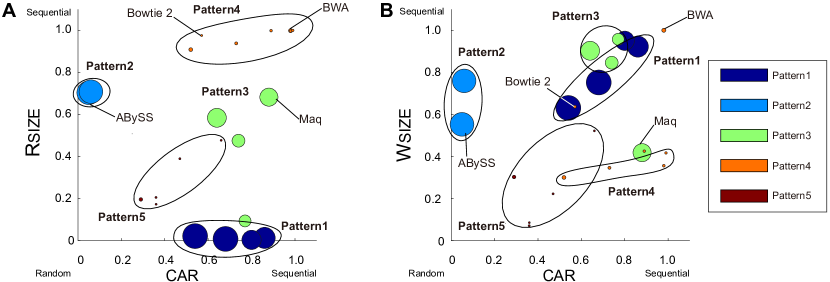
Figure 7: Impact of randomness on speedup. Each circle represents one of the 23 bioinformatics programs listed in Table LABEL:t:tool_list, and its radius is proportional to the amount of speedup achieved by a drop-in replacement. See Figure 5 for pattern definitions. To fully explain the different levels of speedup of different patterns, we need to consider not only randomness but also the other storage features. See the text for details. Discussions on ABySS, Maq, Bowtie 2, and BAW can be found in Section 4. (a) Read. (b) Write. [Rsize, read size per request; Wsize, write size per request; CAR, consecutive access ratio]

3.4 Impact of input size on SSD effectiveness

We hypothesized that even tools that generate a small amount of IOs may benefit from using SSDs as the input size grows. Feeding large data may cause the main memory to be full generating frequent swaps. In this case, using SSDs may help reduce the runtime.

To verify this theory, we tried feeding increasingly larger data to AmpliconNoise [27], a program in P5. Recall that the programs in P5 are not very effectively accelerated by using SSDs, mainly because of their CPU-intensive behavior producing only a small amounts of IOs. The baseline data contains 2000 sequences sampled from the 454 Titanium data [27], and we generated larger data sets by replicating the baseline data. For each data set, we measured the runtime, as shown in Figure 8.

The breakeven point appears after replicating the baseline data five times. After that, using SSDs yields a huge speedup. This experiment confirms our theory and suggests that adopting SSDs may or may not be a smart decision, depending on the size of input data, even for the same program. For instance, AmpliconNoise often handles a number of pyrosequenced reads and is likely to benefit from using SSDs, although AmpliconNoise belongs to P5.

3.5 Effect of main memory size on SSD-based acceleration

The size of main memory affects the runtime of a workload, and ideally, the effect of using SSDs would be eclipsed in a system equipped with the main memory large enough for storing all the input/intermediate/output data. In reality, however, the memory footprint of a bioinformatics workload often becomes significantly larger than the main memory size affordable in typical systems, necessitating the use of a speedy secondary storage, such as SSDs.

We tested how the size of main memory affects the amount of speedup by SSDs using the GATK program, as shown in Figure 9. For an input dataset of 20GB sampled from the NA12878 human whole genome sequence [32], we ran the GATK using three sizes of main memory (4GB, 16GB, and 32GB) and measured the runtime of each of the four subprograms in the GATK for each memory configuration.

Using SSDs was most effective for the sequence base-quality recalibration (GATK BaseRecal) step, which shows high randomness in IO and belongs to P1. For the two memory sizes smaller than the input size (4GB and 16GB main memory), SSDs delivered a significant amount of speedup (66.32 times and 49.79 times, respectively). Even for the 32GB configuration, we observed more than 30 times speedup, which suggests that the memory footprint of GATK BaseRecal grows substantially during execution and the use of SSDs was effective.

For the sequence realignment step (GATK Aligner), the use of SSDs was helpful only for the 4GB memory configuration. For the setups with 16GB and 32GB memory, the amount of speedups was negligible. Although the input file size was 20GB, using SSDs was ineffective for 16GB main memory, which reveals the computing-intensive characteristic of the sequence alignment operation in GATK Aligner and the limited effectiveness of SSDs. For the other two programs (GATK Unified and GATK Printreads), we observed only negligible effects of using SSDs.

3.6 Additional experimental results

In addition to the eight features listed in Table LABEL:t:io_features, which are mostly related to storage devices, we measured CPU- and memory-related features (e.g., CPU usage and cache hit/miss ratios), as shown in Figure 10. The CPU usage was higher for G₀, and the tools therein can be considered more compute-intensive than those in G₊. The miss ratios for the lower-level caches and the translation lookaside buffer (TLB) tend to be higher for G₊, confirming their memory-intensive behavior. The page fault rate was also higher for G₊, which is compatible with the experimental results presented earlier.

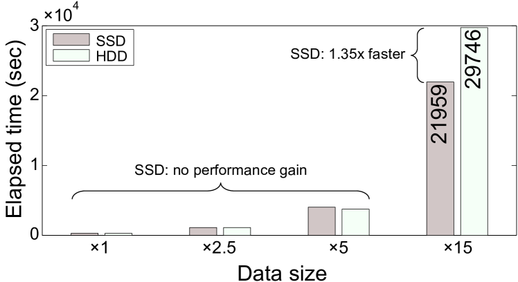
Figure 8: CPU-intensive programs in P5 that produce a small amount of IO for moderate-size data may also benefit significantly by using SSDs for handling very large-scale data. [program: AmpliconNoise [27], baseline data: 2000 reads from 454 Titanium [27]]

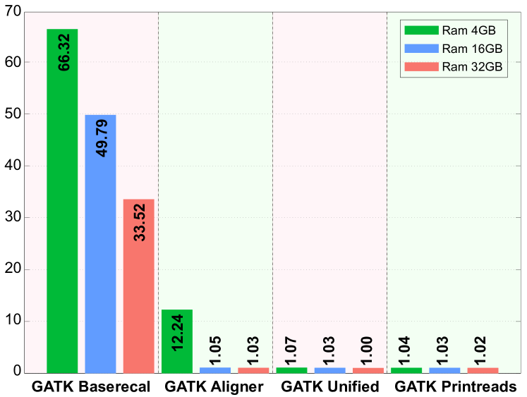
Figure 9: Effects of main memory size on SSD-based acceleration of the GATK [4]. Speedups of each of the four stages of the GATK with three different amounts of main memory are shown. [data: 20GB sample of NA12878 human whole genome sequence [32]]

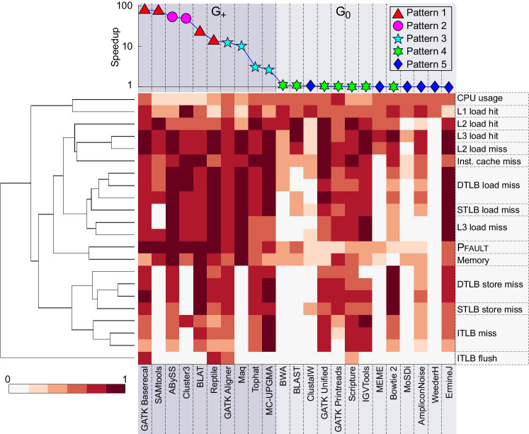
Figure 10: Additional measurements of CPU- and memory-related features for the 23 bioinformatics programs. Speedup of each program is also shown. Features were normalized to values between 0 and 1. [G₊, programs with 2x or more speedup; G₀, programs with negligible improvements]

3.7 Summary and guidelines for employing SSDs in bioinformatics pipelines

As seen in Figure 5(b) and 5(c), the most notable difference between G₊ and G₀  comes from the amount of page faults. In other words, when the memory footprint of a program exceeds the capacity of main memory, using SSDs is likely to bring a significant gain over using HDDs. By contrast, the programs with small memory footprints is less likely to be accelerated by using SSDs.

Optimizing a program by reducing its memory footprint may bring a similar effect as using SSDs, but such a code optimization would typically require a nontrivial amount of efforts. Adopting SSDs thus becomes a more appealing option especially when the resources for code optimization are limited. Installing more main memory would also be helpful for reducing the runtime of programs, but the cost of DRAM may easily become prohibitively expensive, let alone the limited memory bandwidth issue.

Other factors that differentiate G₊ and G₀ include the randomness of IO requests and the amount of data transfers: the more random and larger read/write requests, the more effective the use of SSDs. As the size of input data grows, even some of the programs in G₀ may benefit from using SSDs.

When deploying SSDs in a cluster environment, the administrator of the cluster should consider the network constraints before replacing HDDs with SSDs, because the effect of successful local acceleration may become eclipsed by the network latency, resulting in no overall performance gain (see Section 4 for more details).

4 Discussion

The 23 programs we profiled represent traditional and emerging areas of importance, such as sequence alignment (including conventional dynamic programming-based, heuristic, and BWT-based algorithms), NGS denoising, assembly and mapping (including RNA-seq tools), gene expression analysis, motif finding, variant calling (including four GATK components), and metagenome analysis. These programs should cover the most frequent usages of bioinformatics data processing and related computation.

Through our experiments, we confirmed that acceleration by parallelization can be combined with the use of SSDs for even more performance increases. For example, using SSDs could accelerate ABySS more than 50 times, even though ABySS is a state-of-the-art parallelized assembler. The compute-intensive nature was mitigated by multicore processing, while the data-intensitve nature seems to have been handled by SSDs. The GATK package is another example. GATK was implemented using the map-reduce framework, which is amenable to parallel processing. In our experiments, SSDs could reduce the time demand of the two time-consuming components of GATK (BaseRecal and Aligner) by 78.4 and 12.6 times, respectively. When we design load balancing for parallelization, it will be helpful to consider the amount and randomness of IOs so that we can take advantage of SSDs.

In case the analysis pipeline contains a component program that is not accelerated by using SSDs, replacing the program with an alternative that runs faster on SSDs can help reduce the runtime of the overall pipeline. For example, in the sequence assembly and annotation pipeline depicted in Figure 3(b), replacing Blast (only 1.08x speedup) with Blat (23.6x speedup) gave additional speedup to the whole pipeline. When there are multiple options for selecting a component block in a pipeline, it will thus be beneficial to assess the alternatives in terms of the effectiveness of using SSDs.

To this end, we can consider the three short-read aligners as an example: Maq (hash-based first-generation tool), Bowtie 2 and BWA (BWT-based second-generation tools). These three tools show similar CAR values, although Maq belongs to P3 and Bowtie 2 and BWA both belong to P4. In contrast, there is a difference in the IO size: Maq issues smaller reads but generates larger writes, which are linked to larger values of Pfault and WBlen. When HDDs are used, a critical limitation on the performance of Maq is put. To overcome this issue, significant efforts were made to invent the new generation of tools (Bowtie 2 and BWA) that have smaller memory footprints. The efforts could have been accompanied by using SSDs for even more improvements, given that the page faults and random IOs can be efficiently handled by SSDs.

There remain other intriguing topics for further research. A hybrid drive contains a spacious (but slow) HDD and a speedy (but small) SSD altogether inside a package. The access patterns are monitored, and frequently accessed “hot” data are cached automatically and dynamically in the SSD while the majority of the data are stored in the HDD. Using such a hybrid drive will be helpful for acceleration, under the conditions that the workload program creates enough IO requests (e.g., the programs in group G₊) and the composition of the hot data do not change frequently over time.

Exploiting the redundant array of independent disks (RAID) technology [hennessy2011computer] may provide additional advantages in performance and reliability. In particular, RAID level 0, which consists of striping without mirroring or parity, will be helpful for significantly improving data throughput. As long as the bandwidth of the host interface (e.g., SATA, PCIe, and NVM Express) is high enough to maintain the enhanced data throughput, using SSDs in RAID 0 will be helpful for accelerating high-throughput bioinformatics workloads.

Recently Hadoop-based clusters [taylor2010overview] are popular in large-scale data analytics including bioinformatics. The Hadoop file system (HDFS) provides a distributed storage layer on which various MapReduce-based operations are performed [chen2008map]. The randomness inherently occurring in the Map phase can be effectively handled by using SSDs [moon2014introducing], which are far more superior to HDDs in terms of handling random IO requests. Improving the performance of a namenode (the node managing distributed file systems) in a Hadoop system by SSDs may provide another opportunity for SSD-based acceleration. In distributed systems, however, the network latency often eclipses the speedups achieved locally (e.g., shared-memory-based parallelization and SSD-based acceleration) [appuswamy2013scale], and improving the overall performance globally may require significant efforts. Thus, even if the most frequently used applications in a cluster include the programs in the G+ group, the administrator of the cluster should carefully examine any network constraints that may exist before replacing HDDs with SSDs.

5 Methods

5.1 Experiment setup and measurements

The SSDs and HDDs used in our experiments are listed in Table LABEL:t:ssd_spec and Table LABEL:t:hdd_spec, respectively. We selected these devices because they were the most popular in the market at the time of our experiments. For conservative comparison, the SSDs used are low-end models with 128GB or less capacity, whereas the HDD selection includes high-performance WD VelociRaptor.

Many of the bioinformatics tools we used take a long time to process large data especially when HDDs are used (often in the order of days or even weeks). To compare the performance of HDDs and SSDs using the same data sets while keeping experiments manageable, we selected, for each program, an input data set of appropriate size that can be processed in a reasonable amount of time (the criterion used: less than 72 hours). Table LABEL:t:data_list lists details of the data used to profile the 23 bioinformatics programs.

To see the effects of changing secondary storages clearly in this setup, we also adjusted the specifications of the computer used accordingly. We used a machine equipped with a 3.3GHz Intel Core i3-3220 CPU (4 threads, 4MB L3 cache), 1600MHz dual-channel DDR3 memory (4GB for the GATK tools and 1GB for the others), and Ubuntu 12.04 LTS (Precise Pangolin).

For performance profiling and measurement, we used time (with option -eUSKFW), System Activity Reporter (SAR, [35]), blktrace [36], and Intel VTune Amplifier XE. To avoid interference between tools, we ran each of these profilers independently. We used time and SAR for measuring CPU usage and virtual-memory related features, blktrace for measuring block-level storage features (e.g., read/write amounts, throughput, and IOPS), and VTune for measuring CPU-internal features (e.g., cache hit/miss, TLB hit/miss, and IPC). When the range of measurements was large, we took the logarithm. We then normalized each of the measurements so that values were ranged in $[0,1]$. We repeated all the time measurements three times and used the average value for the analysis.

[ caption = Specifications of the SSDs used in this work, label = t:ssd_spec, ]lrrrrrr SSD Capacity Sequential (MB/s) Random (IOPS)
(GB) Read Write Read Write
Samsung 830 128 520 320 80,00030,000
Samsung 840 Pro 128 530 39097,00090,000
OCZ Vertex4 128 560 43090,00085,000
Intel 520 120 550 47550,00080,000
Plextor M5 Pro 128 540 33091,00082,000
Corsair Neutron GTX 120 555 330 85,00084,000

[ caption = Specifications of the HDDs used in this work, label = t:hdd_spec, ]lrrrrrrrr HDD Capacity RPM Buffer size Read/write IOPS (estimated)
(GB) (MB) (MB/s) ReadWrite
Seagate Barracuda 1,000 7,200 64 156 79.0 73.2
WD Caviar Blue 1,000 7,200 64 15076.6 66.4
WD VelociRaptor 500 10,000 64 200151.5 138.9

[ caption = List of the data used to test the 23 programs listed in Table LABEL:t:tool_list, label = t:data_list, ]lll []$\dagger$ftp://ftp-trace.ncbi.nih.gov/1000genomes/ftp/technical/working/20101201_cg_NA12878/; $\ddagger$http://trace.ddbj.nig.ac.jp/DRASearch/submission?acc=SRA012173; $\sharp$ftp://ftp.ncbi.nih.gov/pub/geo/DATA/supplementary/series/GSE20851/GSE20851_GSM521650_ES.aligned.sam.gz;  $\S$http://www.ncbi.nlm.nih.gov/geo/query/acc.cgi?acc=GPL92 Program Data Source
GATK BaseRecal NA12878 human link^†
Samtools C2 [37]
ABySS Staphyloccus aureus [31]
Cluster3 Protein structure [38]
Blat NCBI Uniref50 protein [39]
Reptile Human chromosome 14 [31]
GATK AlignerNA12878 human link^†
Maq Human chromosome 14 [31]
Tophat Drosophila melanogaster link^‡
MC-UPGMA Protein structure [38]
BWA AT1 [37]
Blast NCBI Uniref50 protein [39]
ClustalW NCBI Uniref50 protein [39]
GATK UnifiedNA12878 human link^†
GATK PrintReadsNA12878 human link^†
Scripture Mouse (mm9) reads link^♯
IGVtools Mouse (mm9) reads link^♯
Meme Human sequence hm01 [40]
Bowtie 2AT1 [37]
Mosdi Human sequence hm01 [40]
AmpliconNoise 454 Titanium [27]
WeederHuman sequence hm01 [40]
ErmineJHuman genome U95 set link^§

5.2 More details of the storage features used

Recall that we profile and analyze the 23 programs in terms of eight storage features that can characterize the amount and/or randomness of IOs.

To measure the amount of IOs we use three measures. Butil measures how much bandwidths of the interface between the host computer and the storage device are used. If there is a large amount of data transfers between the host and storage, Butilwould be high. Riops and Wiops measure how many read and write requests are made per second, respectively. A high value of these features implies frequent read/write requests. Pfault represents the number of page swaps per second. High Pfault suggests frequent page swaps, which can be costly for HDDs.

The randomness of IOs can be measured in different ways. In this paper, we use two widely used measures: read/write size per request [41] and Consecutive Access Ratio (CAR, [42]). Reads or writes that transfer a small amount of data are often considered random, whereas large read/write transfers are considered sequential. CAR measures how often consecutive accesses to the LBA space occur. The CAR value of one (zero) means perfectly sequential (random) IO access patterns.

WBlen represents the number of write requests waiting in the write buffer of a storage device. High WBlen normally can be caused by a high amount of write IOs and/or by a large number of small random writes. WBlen is thus related to both the amount and the randomness of IOs.

6 Conclusion

There exist cases in which a simple drop-in replacement of HDDs by SSDs can dramatically expedite bioinformatics programs. For instance, we observed more than 50 times speedup of widely used tools, such as GATK components, Samtools, and ABySS. In the arena of short-read aligners, we observed that Maq (a hash-based first-generation tool) could compete again with Bowtie 2 and BWA (the second-generation tools) leveraged by SSDs. According to our experiments, using SSDs could accelerate the GATK-based variant calling pipeline by more than 30 times.

However, SSDs are not silver bullets and cannot boost every bioinformatics program of one’s interest. Moreover, SSDs are still expensive. Eventually the price of SSDs may become competitive to HDDs, but the price per gigabyte of SSDs is still approximately 15 times more expensive, as of 2015. Researchers handling large-scale biomedical data should thus make a careful and informed decision regarding whether to replace their HDDs (at least partially) with SSDs.

To this end, profiling the bioinformatics tools of interest from system perspectives is critical. According to our experiments, there exist many bioinformatics programs that can benefit immediately by using SSDs, especially when the program causes frequent random IOs or page swaps due to relatively large input compared to system memory. This review reports other patterns indicating the viability of SSD-based acceleration. As the size of input data grows, we expect that the territory of the SSD-acceleratable programs will expand.

In any case, as the performance of SSDs is rapidly improving with continuous cost reduction and technology developments, SSDs will eventually become the storage device of choice, phasing out HDDs firstly in performance-critical domains and later in the mainstream. We thus believe that future bioinformatics algorithms should be designed to consider the advantage of using SSDs in addition to the applicability of parallel processing. We hope that the results and insight presented in this review will be a valuable asset to such a journey for inventing efficient and scalable bioinformatics tools.

References

- [1] E. E. Schadt, “The changing privacy landscape in the era of big data,” Molecular systems biology, vol. 8, no. 1, 2012.
- [2] A. Holzinger, Biomedical Informatics: Discovering Knowledge in Big Data. Springer, 2014.
- [3] J. Lee, W. Kladwang, M. Lee, D. Cantu, M. Azizyan, H. Kim, A. Limpaecher, S. Yoon, A. Treuille, and R. Das, “Rna design rules from a massive open laboratory,” Proceedings of the National Academy of Sciences, vol. 111, no. 6, pp. 2122–2127, 2014.
- [4] A. McKenna et al., “The genome analysis toolkit: a mapreduce framework for analyzing next-generation dna sequencing data,” Genome research, vol. 20, no. 9, pp. 1297–1303, 2010.
- [5] R. Balasubramonian et al., “Near-data processing: Insights from a micro-46 workshop,” Micro, IEEE, vol. 34, no. 4, pp. 36–42, 2014.
- [6] R. H. Katz et al., Disk system architectures for high performance computing. University of California, Berkeley, Computer Science Division, 1989.
- [7] B. Seo, S. Kang, J. Choi, J. Cha, Y. Won, and S. Yoon, “IO workload characterization revisited: A data-mining approach,” IEEE Transactions on Computers, vol. 63, no. 12, pp. 3026–3038, 2014.
- [8] S.-W. Lee et al., “A case for flash memory SSD in enterprise database applications,” in Proceedings of the 2008 ACM SIGMOD international conference on Management of data, pp. 1075–1086, ACM, 2008.
- [9] J. T. Simpson, K. Wong, S. D. Jackman, J. E. Schein, S. J. Jones, and İ. Birol, “Abyss: a parallel assembler for short read sequence data,” Genome research, vol. 19, no. 6, pp. 1117–1123, 2009.
- [10] J. Dean and S. Ghemawat, “Mapreduce: simplified data processing on large clusters,” Communications of the ACM, vol. 51, no. 1, pp. 107–113, 2008.
- [11] M. L. Metzker, “Sequencing technologies—the next generation,” Nature Reviews Genetics, vol. 11, no. 1, pp. 31–46, 2009.
- [12] H. Li, J. Ruan, and R. Durbin, “Mapping short dna sequencing reads and calling variants using mapping quality scores,” Genome research, vol. 18, no. 11, pp. 1851–1858, 2008.
- [13] H. Li and R. Durbin, “Fast and accurate short read alignment with burrows–wheeler transform,” Bioinformatics, vol. 25, no. 14, pp. 1754–1760, 2009.
- [14] B. Langmead and S. L. Salzberg, “Fast gapped-read alignment with bowtie 2,” Nature methods, vol. 9, no. 4, pp. 357–359, 2012.
- [15] H. Li, B. Handsaker, A. Wysoker, T. Fennell, J. Ruan, N. Homer, G. Marth, G. Abecasis, R. Durbin, et al., “The sequence alignment/map format and samtools,” Bioinformatics, vol. 25, no. 16, pp. 2078–2079, 2009.
- [16] M. J. de Hoon, S. Imoto, J. Nolan, and S. Miyano, “Open source clustering software,” Bioinformatics, vol. 20, no. 9, pp. 1453–1454, 2004.
- [17] W. J. Kent, “Blat—the blast-like alignment tool,” Genome research, vol. 12, no. 4, pp. 656–664, 2002.
- [18] X. Yang, K. S. Dorman, and S. Aluru, “Reptile: representative tiling for short read error correction,” Bioinformatics, vol. 26, no. 20, pp. 2526–2533, 2010.
- [19] C. Trapnell, L. Pachter, and S. L. Salzberg, “Tophat: discovering splice junctions with rna-seq,” Bioinformatics, vol. 25, no. 9, pp. 1105–1111, 2009.
- [20] Y. Loewenstein, E. Portugaly, M. Fromer, and M. Linial, “Efficient algorithms for accurate hierarchical clustering of huge datasets: tackling the entire protein space,” Bioinformatics, vol. 24, no. 13, pp. i41–i49, 2008.
- [21] S. F. Altschul, W. Gish, W. Miller, E. W. Myers, and D. J. Lipman, “Basic local alignment search tool,” Journal of molecular biology, vol. 215, no. 3, pp. 403–410, 1990.
- [22] J. D. Thompson et al., “CLUSTAL W: improving the sensitivity of progressive multiple sequence alignment through sequence weighting, position-specific gap penalties and weight matrix choice,” Nucleic acids research, vol. 22, no. 22, pp. 4673–4680, 1994.
- [23] M. Guttman et al., “Ab initio reconstruction of cell type-specific transcriptomes in mouse reveals the conserved multi-exonic structure of lincrnas,” Nature biotechnology, vol. 28, no. 5, pp. 503–510, 2010.
- [24] J. T. Robinson and othes, “Integrative genomics viewer,” Nature biotechnology, vol. 29, no. 1, pp. 24–26, 2011.
- [25] T. L. Bailey et al., “Meme: discovering and analyzing dna and protein sequence motifs,” Nucleic acids research, vol. 34, no. suppl 2, pp. W369–W373, 2006.
- [26] T. Marschall and S. Rahmann, “Efficient exact motif discovery,” Bioinformatics, vol. 25, no. 12, pp. i356–i364, 2009.
- [27] C. Quince, A. Lanzen, R. J. Davenport, and P. J. Turnbaugh, “Removing noise from pyrosequenced amplicons,” BMC bioinformatics, vol. 12, no. 1, p. 38, 2011.
- [28] G. Pavesi et al., “Weederh: an algorithm for finding conserved regulatory motifs and regions in homologous sequences,” BMC bioinformatics, vol. 8, no. 1, p. 46, 2007.
- [29] J. Gillis, M. Mistry, and P. Pavlidis, “Gene function analysis in complex data sets using erminej,” Nature protocols, vol. 5, no. 6, pp. 1148–1159, 2010.
- [30] P. Flicek and E. Birney, “Sense from sequence reads: methods for alignment and assembly,” Nature methods, vol. 6, pp. S6–S12, 2009.
- [31] S. L. Salzberg, A. M. Phillippy, A. Zimin, D. Puiu, T. Magoc, S. Koren, T. J. Treangen, M. C. Schatz, A. L. Delcher, M. Roberts, et al., “Gage: A critical evaluation of genome assemblies and assembly algorithms,” Genome research, vol. 22, no. 3, pp. 557–567, 2012.
- [32] 1000 Genomes Project Consortium, “A map of human genome variation from population-scale sequencing,” Nature, vol. 467, no. 7319, pp. 1061–1073, 2010.
- [33] I. Birol et al., “De novo transcriptome assembly with abyss,” Bioinformatics, vol. 25, no. 21, pp. 2872–2877, 2009.
- [34] A. Mortazavi et al., “Mapping and quantifying mammalian transcriptomes by rna-seq,” Nature methods, vol. 5, no. 7, pp. 621–628, 2008.
- [35] C.-D. Lu et al., “Comprehensive job level resource usage measurement and analysis for xsede hpc systems,” in Proceedings of the Conference on Extreme Science and Engineering Discovery Environment, p. 50, ACM, 2013.
- [36] A. D. Brunelle, “Blktrace user guide,” 2007.
- [37] A. K. Bartram et al., “Generation of multimillion-sequence 16s rrna gene libraries from complex microbial communities by assembling paired-end illumina reads,” vol. 77, no. 11, pp. 3846–3852, 2011.
- [38] S. Yoon, J. C. Ebert, E.-Y. Chung, G. De Micheli, and R. B. Altman, “Clustering protein environments for function prediction: finding prosite motifs in 3d,” BMC bioinformatics, vol. 8, no. Suppl 4, p. S10, 2007.
- [39] UniProt Consortium, “The universal protein resource (uniprot) in 2010,” Nucleic acids research, vol. 38, no. suppl 1, pp. D142–D148, 2010.
- [40] M. Tompa et al., “Assessing computational tools for the discovery of transcription factor binding sites,” Nature biotechnology, vol. 23, no. 1, pp. 137–144, 2005.
- [41] C. Li et al., “Assert (! defined (sequential i/o)),” in Proceedings of the 6th USENIX conference on Hot Topics in Storage and File Systems, pp. 10–10, 2014.
- [42] A. Traeger, E. Zadok, N. Joukov, and C. P. Wright, “A nine year study of file system and storage benchmarking,” ACM Transactions on Storage (TOS), vol. 4, no. 2, p. 5, 2008.