Compactly Supported One-cyclic Wavelets Derived from Beta Distributions

Resumo

New continuous wavelets of compact support are introduced, which are related to the beta distribution. They can be built from probability distributions using ”blur”derivatives. These new wavelets have just one cycle, so they are termed unicycle wavelets. They can be viewed as a soft variety of Haar wavelets whose shape is fine-tuned by two parameters $a$ and $b$. Close expressions for beta wavelets and scale functions as well as their spectra are derived. Their importance is due to the Central Limit Theorem applied for compactly supported signals.

I PRELIMINARIES AND BACKGROUND

Wavelets are strongly connected with probability distributions. Recently, a new insight into wavelets was presented, which applies Max Born reading for the wave-function [1] in such a way that an information theory focus has been achieved [2]. Many continuous wavelets are derived from a probability density (e.g. Sombrero). This approach also sets up a link among probability densities, wavelets and “blur derivatives” [3]. To begin with, let $P(.)$ be a probability density, $P\in\mathbb{C}^{\infty}$, the space of complex signals $f:\mathbb{R}\rightarrow\mathbb{C}$ infinitely differentiable.

If

$$\stackrel{{\scriptstyle\lim}}{{{}_{t\rightarrow\infty}}}\frac{d^{n-1}P(t)}{dt^{n-1}}=0$$ (1)

then

$$\psi(t)=(-1)^{n}\frac{d^{n}P(t)}{dt^{n}}$$ (2)

is a wavelet engendered by $P(.)$. Given a mother wavelet $\psi$ that holds the admissibility condition [4,5] then the continuous wavelet transform is defined by

$$CWT(a,b)=\int^{+\infty}_{-\infty}f(t)\cdot\frac{1}{\sqrt{|a|}}\psi(\frac{t-b}{a})dt,$$ (3)

$\forall a\in\mathbb{R}-\{0\}$, $b\in\mathbb{R}$.

Continuous wavelets have often unbounded support, such as Morlet, Meyer, Mathieu, de Oliveira wavelets [6-8]. In the case where the wavelet was generated from a probability density, one has

$$\frac{1}{\sqrt{|a|}}\psi_{n}(\frac{t-b}{a})=(-1)^{n}\frac{1}{\sqrt{|a|}}\frac{\partial^{n}P(\frac{t-b}{a})}{\partial t^{n}}.$$ (4)

Now

$$\frac{\partial^{n}P(\frac{t-b}{a})}{\partial b^{n}}=(-1)^{n}\frac{1}{a^{n}}P^{(n)}(\frac{t-b}{a}),$$ (5)

so that

$$CWT(a,b)=\frac{1}{\sqrt{|a|}}\int^{+\infty}_{-\infty}f(t)\cdot\frac{\partial^{n}P(\frac{t-b}{a})}{\partial b^{n}}dt.$$ (6)

If the order of the integral and derivative can be commuted, it follows that

$$CWT(a,b)=\frac{1}{\sqrt{|a|}}\frac{\partial^{n}}{\partial b^{n}}\int^{+\infty}_{-\infty}f(t)\cdot P(\frac{t-b}{a})dt.$$ (7)

Defining the LPFed signal as the ”blur”signal

$$\widetilde{f}(a,b)=\int^{+\infty}_{-\infty}f(t)\cdot\frac{1}{\sqrt{|a|}}P(\frac{t-b}{a})dt=\int^{+\infty}_{-\infty}f(t)\cdot P_{a,b}(t)dt,$$ (8)

an interesting interpretation can be made: set a scale $a$ and take the average (smoothed) version of the original signal - the blur version $\widetilde{f}(a,b)$. The “blur derivative”

$$\frac{\partial^{n}}{\partial b^{n}}\widetilde{f}(a,b)$$ (9)

is the $n^{th}$ derivative regarding the shift $b$ of the blur signal at the scale $a$. The blur derivative coincide with the wavelet transform $CWT(a,b)$ at the corresponding scale. Details (high-frequency) are provided by the derivative of the low-pass (blur) version of the original signal.

I-A Revisiting Central Limit Theorems

There are essentially three kinds of central limit theorems: for unbounded distributions, for causal distributions and for compactly supported distributions [9]. The random variable corresponding to the sum of $N$ independent and identically distributed (i.i.d.) variables converges to: a Gaussian distribution, a Chi-square distribution or a Beta distribution (see Table I). The Gaussian pulse always has been playing a very central role in Engineering and it is associated with Morlet’s wavelet, which is known to be of unbounded support. This is the only wavelet that meets the lower bound of Gabor’s uncertainty inequality [10]. The Gabor concept of logon naturally leads to the Gaussian waveforms as an efficient signalling in the time-frequency plan. Nevertheless, in the cases where a constraint in signal duration is imposed, it can be expected that beta waveforms will be the most efficient signalling in the time-frequency plan. The concept of wavelet entropy was recently introduced and Morlet wavelet also revealed to be a special wavelet [2,11]. Among all wavelets of compact support, it can be expected that the one linked to the beta distribution could also play a valuable practical and theoretical role.

Tabela I: DIFFERENT VERSIONS OF THE CENTRAL LIMIT THEOREM: UNBOUNDED DISTRIBUTIONS, CAUSAL DISTRIBUTIONS AND COMPACTLY SUPPORTED PROBABILITY DISTRIBUTIONS.

Marginal Distribution	Central Limit Distribution as $N\rightarrow\infty$
Unbounded Support	$G(t|m,\sigma^{2})=\frac{1}{sqrt{2\pi\sigma^{2}}}\cdot e^{\frac{-(t-m)^{2}}{2\sigma^{2}}}$
Causal Distribution	$\chi^{2}(t|m,\sigma^{2})=\frac{t^{\alpha}\cdot\beta^{-t\diagup\beta}}{\beta^{\alpha+1}\Gamma(\alpha+1)}$
Compact Support	$beta(t|\alpha,\beta)=K\cdot t^{\alpha}\cdot(1-t)^{\beta},\quad 0<t<1$

Let $p_{i}(t)$ be a probability density of the random variable $t_{i}$,where $i=1,2,3..N$ i.e. $p_{i}(t)\geqslant 0$ , $(\forall t)$ and

$$\int^{+\infty}_{-\infty}p_{i}(t)dt=1.$$ (10)

If $p_{i}(t)\leftrightarrow P_{i}(\omega)$ , then $P_{i}(0)=1$ and $(\forall\omega)|P_{i}(\omega)|\leq 1$ . Suppose that all variables are independent. The density $p(t)$ of the random variable corresponding to the sum

$$t=\sum^{N}_{i=1}t_{i}$$ (11)

is given by the iterate convolution [12]

$$p(t)=p_{1}(t)*p_{2}(t)*p_{3}(t)*...p_{N}(t).$$ (12)

If $p_{i}(t)\leftrightarrow P_{i}(\omega)=|P_{i}(\omega)|e^{j\Theta_{i}(\omega)}$, $i=1,2,3..N$ and $p(t)\leftrightarrow P(\omega)=|P(\omega)|e^{j\Theta(\omega)}$ , then

$$|P(\omega)|=\prod^{N}_{i=1}|P_{i}(\omega)|,\qquad\Theta(\omega)=\sum^{N}_{i=1}\Theta_{i}(\omega).$$ (13)

The mean and the variance of a given random variable $t_{i}$ are, respectively

$$m_{i}=\int^{+\infty}_{-\infty}\tau\cdot p_{i}(\tau)d\tau,$$ (14)

$$\sigma^{2}_{i}=\int^{+\infty}_{-\infty}(\tau-m_{i})^{2}\cdot p_{i}(\tau)d\tau.$$ (15)

The following theorems can be proved [9].

Theorem 1

Central Limit Theorem for distributions of unbounded support
If the distributions $\{p_{i}(t)\}$ are not a lattice (a Dirac comb) and $E(t^{3}_{i})<\infty$, and

$$\lim_{N\rightarrow\infty}\sigma^{2}=+\infty$$

then $t=\sum^{N}_{i=1}t_{i}$ holds, as $N\rightarrow\infty$,

$$P(\omega)\sim e^{-{\frac{\sigma^{2}\omega^{2}}{2}}-jm\omega},$$ (16)

$$p(t)\sim\frac{1}{\sqrt{2\pi\sigma^{2}}}e^{-{\frac{(t-m)^{2}}{2\sigma^{2}}}}$$ (17)

$\Box$

According to Gnedenko and Kolmogorov, if all marginal probability densities have bounded support, then the corresponding theorem is [9]:

Theorem 2

Central Limit Theorem for distributions of compact support. Let $\{p_{i}(t)\}$ be distributions such that $Supp\{(p_{i}(t))\}=(a_{i},b_{i})(\forall i)$. Let

$$a=\sum^{N}_{i=1}a_{i}<+\infty,$$ (18)

$$b=\sum^{N}_{i=1}b_{i}<+\infty.$$ (19)

It is assumed without loss of generality that $a=0$ and $b=1$. The random variable defined by (11) holds as $N\rightarrow\infty$,

$$p(t)\sim\Biggl{\{}\begin{array}[]{rcl}k\cdot t^{\alpha}(1-t)^{\beta},&0\leq t\leq 1\\ 0,&\mbox{otherwise}\end{array}$$ (20)

where

$$\alpha=\frac{m(m-m^{2}-\sigma^{2})}{\sigma^{2}},$$ (21)

and

$$\beta=\frac{(1-m)(\alpha+1)}{m}.$$ (22)

$\Box$

In spite of the fact that a general theory of deriving wavelets from probability distributions is well known, the particular application discussed in this paper search for discovering a link between the most noteworthy compact support distribution and wavelets.

II $\beta$-WAVELETS: NEW COMPACTLY SUPPORTED WAVELETS

The beta distribution is a continuous probability distribution defined over the interval $0\leq t\leq 1$ [13]. It is characterized by a couple of parameters, namely $\alpha$ and $\beta$, according to:

$$P(t)=\frac{1}{B(\alpha,\beta)}t^{\alpha-1}\cdot(1-t)^{\beta-1},\quad 1\leq\alpha,\beta\leq+\infty.$$ (23)

The normalizing factor is $B(\alpha,\beta)=\frac{\Gamma(\alpha)\cdot\Gamma(\beta)}{\Gamma(\alpha+\beta)}$, where $\Gamma(\cdot)$ is the generalized factorial function of Euler and $B(\cdot,\cdot)$ is the Beta function [13].

The following parameters can be computed:

$$Supp{(P)}=[0,1]$$ (24)

$$mean=\frac{\alpha}{\alpha+\beta}$$ (25)

$$mode=\frac{\alpha-1}{\alpha+\beta-2}$$ (26)

$$variance=\sigma^{2}=\frac{\alpha\beta}{(\alpha+\beta)^{2}(\alpha+\beta+1)}$$ (27)

$$characteristicfunction=M(\alpha,\alpha+\beta,j\nu),$$ (28)

where $M(\cdot,\cdot,\cdot)$ is the Kummer confluent hypergeometric function [14, 15]. The $N^{th}$ moment of $P(\cdot)$ can be found using

$$moment(N)=\int^{1}_{0}t^{N}\cdot p_{i}(t)dt=\frac{B(\alpha+N,\beta)}{B(\alpha,\beta)}$$

$$=\frac{B(\alpha+\beta,N)}{B(\alpha,N)}.$$ (29)

The derivative of the beta distribution can easily be found.

$$P^{\prime}(t)=\Bigl{(}\frac{\alpha-1}{t}-\frac{\beta-1}{1-t}\Bigl{)}P(t).$$ (30)

A random variable transform can be made by an affine transform in order to generate a new distribution with zero-mean and unity variance [12], which implies a non-normalized support $T=\frac{1}{\sigma}=T(\alpha,\beta)$.
Let a new random variable be defined by $T\cdot(t-m)$. This variable has zero-mean and unity variance. Its corresponding probability density is given by

$$P(t|\alpha,\beta)=\frac{1}{B(\alpha,\beta)T(\alpha,\beta)}\Bigl{(}\frac{t+m(\alpha,\beta)T(\alpha,\beta)}{T(\alpha,\beta)}\Bigl{)}^{\alpha-1}\cdot$$

$$\Bigl{(}1-\frac{t+m(\alpha,\beta)T(\alpha,\beta)}{T(\alpha,\beta)}\Bigl{)}^{\beta-1}.$$ (31)

The $\beta$-wavelets can now be derived from these modified distributions by using the concept of ”blur”derivative. The (unimodal) scale function associated with the wavelets is given by

$$\phi_{beta}(t|\alpha,\beta)=\frac{1}{B(\alpha,\beta)T^{\alpha+\beta-1}}\cdot(t-a)^{\alpha-1}\cdot(b-t)^{\beta-1},$$ (32)

$a\leq t\leq b$. Since $P(\cdot|\alpha,\beta)$ is unimodal, the wavelet generated by

$$\psi_{beta}(t|\alpha,\beta)=(-1)\frac{dP(t|\alpha,\beta)}{dt}$$ (33)

has only one-cycle (a negative half-cycle and a positive half-cycle).
A close expression for first-order beta wavelets can easily be derived. Within the support of $\psi(t|\alpha,\beta),\quad a\leq t\leq b$,

$$\psi_{beta}(t|\alpha,\beta)=\frac{-1}{B(\alpha,\beta)T^{\alpha+\beta-1}}\cdot\Bigl{[}\frac{\alpha-1}{t-a}-\frac{\beta-1}{b-t}\Bigl{]}\cdot$$

$$(t-a)^{\alpha-1}\cdot(b-t)^{\beta-1}$$ (34)

As a particular case, symmetric beta wavelets are given by

$$\psi_{beta}(t|\alpha,\alpha)=K(\alpha)\cdot t\cdot[t^{2}-(2\alpha+1)]^{\alpha-2},$$ (35)

where

$$K(\alpha)=(-1)^{\alpha}\cdot\frac{2(\alpha-1)}{(2\sqrt{2\alpha+1})^{2\alpha-1}}\cdot\frac{\Gamma(2\alpha)}{[\Gamma(\alpha)]^{2}}.$$ (36)

The main features of beta wavelets of parameters $\alpha$ and $\beta$ are:

$$Supp(\psi) = \Bigl{[}\frac{-1}{\sqrt{{\beta}\diagup{\alpha}}}\sqrt{\alpha+\beta+1},\sqrt{\frac{\beta}{\alpha}}\sqrt{\alpha+\beta+1}\Bigl{]}$$ (37)

$$= [a,b]$$

$$lengthSupp(\psi)=T(\alpha,\beta)=(\alpha+\beta)\sqrt{\frac{\alpha+\beta+1}{\alpha\beta}}.$$ (38)

The parameter $R=b\diagup|a|=\beta\diagup\alpha$ is referred to as ”cyclic balance”, and is defined as the ratio between the lengths of the causal and non-causal piece of the wavelet. It can be easily shown that the instant of transition $t_{zerocross}$ from the first to the second half cycle is given by

$$t_{zerocross}=\frac{(\alpha-\beta)}{(\alpha+\beta-2)}\sqrt{\frac{\alpha+\beta+1}{\alpha\beta}}.$$ (39)

Although scale and wavelets can be found for any $\alpha,\beta>1$, the behavior of the wavelet at the extreme points of the support can be discontinuous (e.g. see Table Ia). However, it is a simple matter to guarantee the continuity of the wavelet according to:

Proposition 1

Beta one-cycle wavelets of parameters $\alpha>2$ and $\beta>2$ are smooth, continuous wavelets of compact support.

Proof:

Clearly, $\psi_{beta}(t|\alpha,\beta)=0\quad\forall t<a$ and $\forall t>b$. The only concerns are therefore with the extreme points of the support, but $\psi_{beta}(a|\alpha,\beta)=\psi_{beta}(b|\alpha,\beta)=0$ provided that $\alpha>2$ and $\beta>2.$ ∎

Remember that $1\leq\alpha,\beta\leq+\infty$ and $a<0<b$.
The beta wavelet spectrum can be derived in terms of the Kummer hypergeometric function [14], which is solution of the equation

$$z\frac{d^{2}\omega}{dz}+(\beta-z)\frac{d\omega}{dz}-\alpha\omega=0.$$ (40)

Let $\psi_{beta}(t|\alpha,\beta)\leftrightarrow\Psi_{BETA}(\omega|\alpha,\beta)$ denote the Fourier transform pair associated with the wavelet. This spectrum is also denoted by $\Psi_{BETA}(\omega)$ for short. It can be proved by applying properties of the Fourier transform that

$$\Psi_{BETA}(\omega) =-j\omega\cdot M\Bigl{(}\alpha,\alpha+\beta,-j\omega(\alpha+\beta)\sqrt{\frac{\alpha+\beta+1}{\alpha\beta}}\Bigl{)}\cdot$$ (41)

$$exp{(j\omega\sqrt{\frac{\alpha(\alpha+\beta+1)}{\beta}})}.$$

The spectrum of a number of unicyclic beta wavelets is presented in Figure 1. The spectrum evaluation was carried out using the relationship:

$$M(\alpha,\alpha+\beta,j\nu)=\frac{\Gamma(\alpha+\beta)}{\Gamma(\alpha)\cdot\Gamma(\beta)}\cdot\int^{1}_{0}e^{j\nu t}t^{\alpha-1}(1-t)^{\beta-1}dt$$ (42)

Only symmetrical $(\alpha=\beta)$ cases have zeroes in the spectrum (Fig. 1a). A few asymmetric $(\alpha\neq\beta)$ beta wavelets are shown in Fig. 1b. Inquisitively, they are parameter-symmetrical in the sense that they hold

$$|\Psi_{BETA}(\omega|\alpha,\beta)|=|\Psi_{BETA}(\omega|\beta,\alpha)|.$$ (43)

The spectrum of symmetric beta wavelets has been compared to that of Haar wavelets of same support, just to check on the reliability of spectral computations. The first spectral null of a Haar wavelet of support $T(\alpha,\beta)$ occurs at a frequency $\omega_{0}=\frac{2\pi}{T(\alpha,\beta)\diagup 2}$ or $\nu_{0}=4\pi$, then at $6\pi,8\pi$ etc. For $\alpha=3$, the first spectral null occurred at a frequency $\nu=11.526918406...$, which is close to $\nu_{0}=4\pi$ as expected. As $\alpha$ increases, the wavelet half-cycle tends to be shrunk (e.g. fig.2 b and e), thereby increasing the frequency of the first spectral notch (Fig.1a).

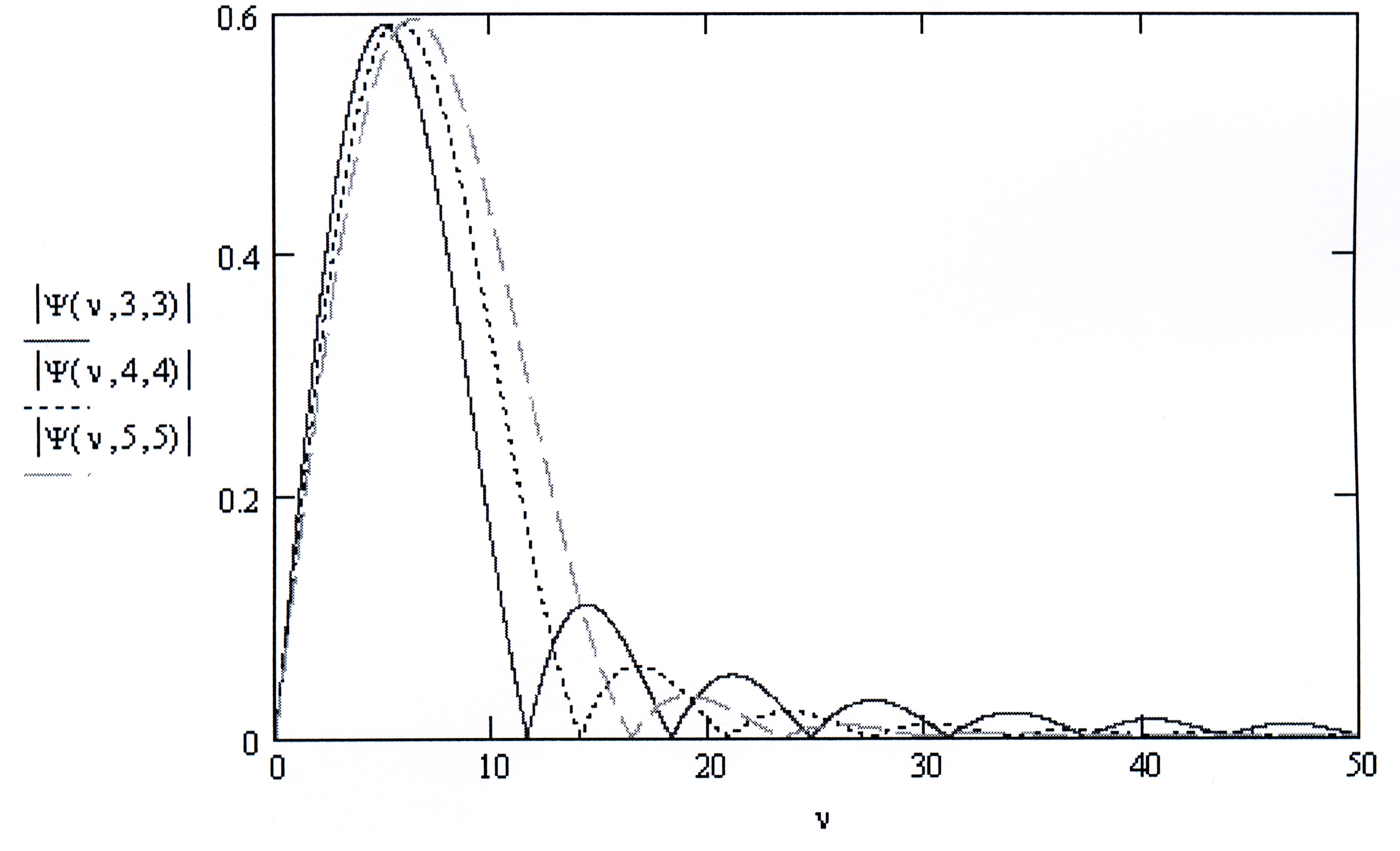
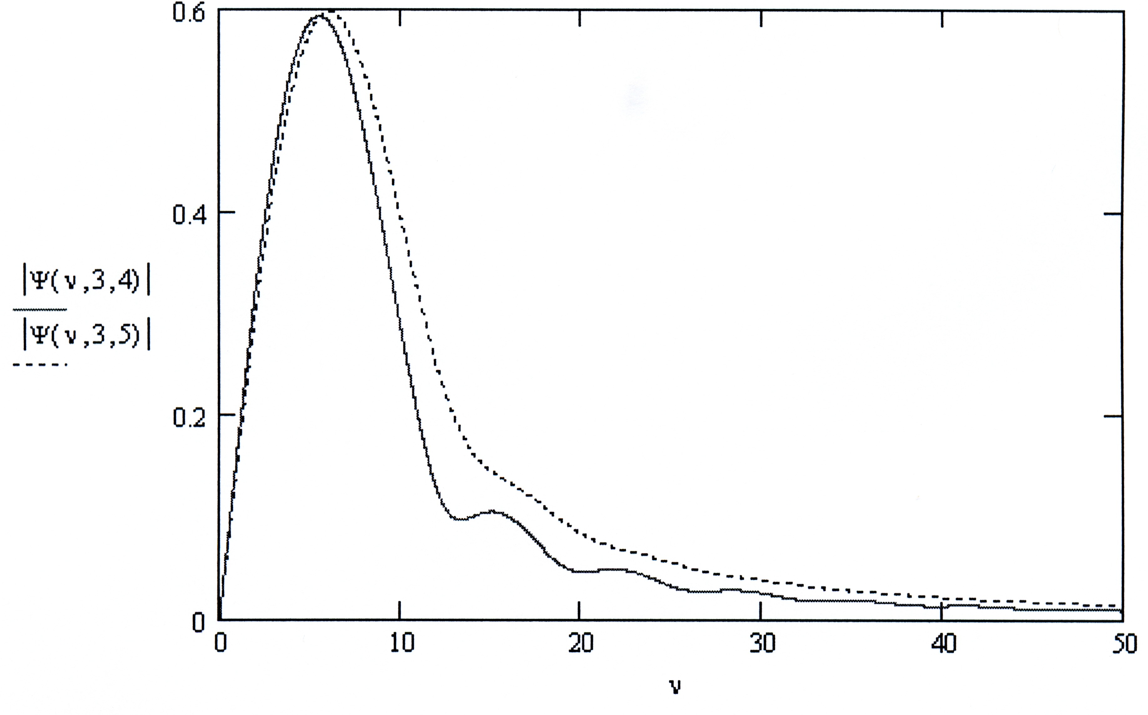
Figura 1: Magnitude of the spectrum $\Psi_{BETA}(\omega)$ of a few beta wavelets, $|\Psi_{BETA}(\nu|\alpha,\beta)|\times\nu$ for: a) symmetric beta wavelets $\alpha=\beta=3$ (solid), $\alpha=\beta=4$(dot) and $\alpha=\beta=5$ (dash); b) asymmetric beta wavelets $\alpha=3$, $\beta=4$ (solid) and $\alpha=3$, $\beta=5$ (dot). In both plots the frequency axis is a normalized spectral frequency $\nu=\omega T(\alpha,\beta)$.

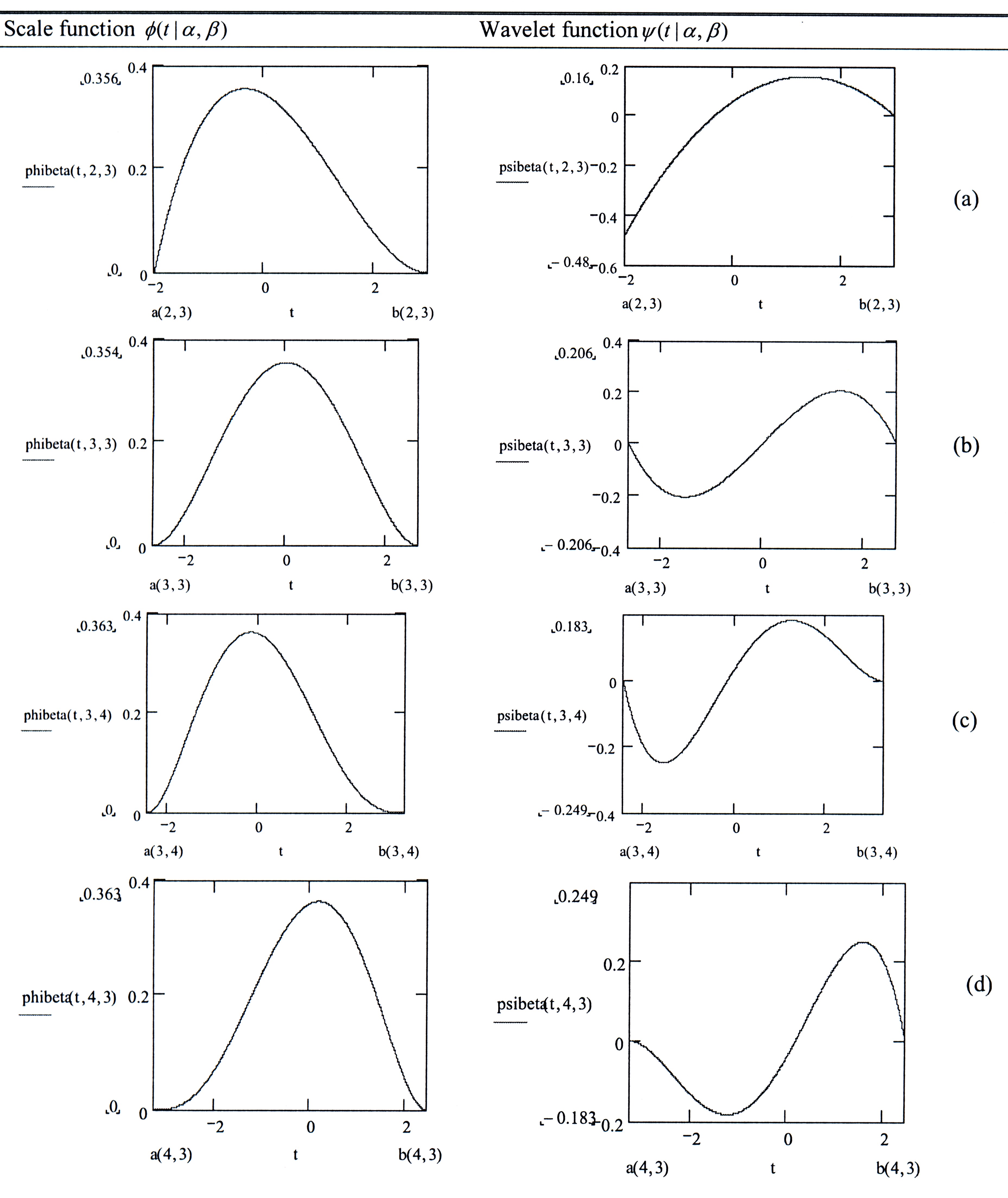
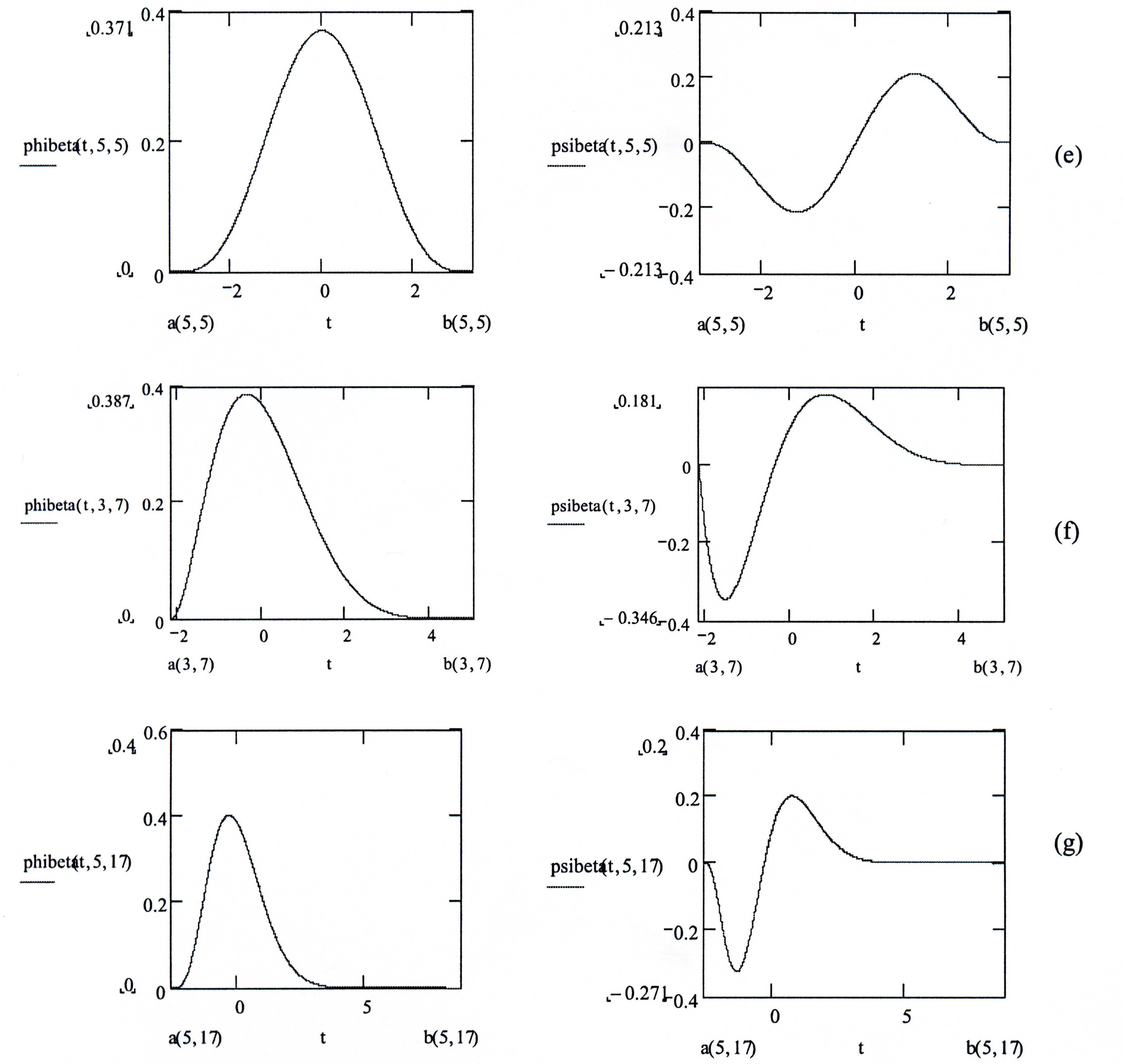
Figura 2: Unicycle-beta scale function and wavelet for different parameters:a) $\alpha=2,\beta=3$ b) $\alpha=\beta=3$ c) $\alpha=3,\beta=4$ d) $\alpha=4,\beta=3$ e) $\alpha=\beta=5$ f) $\alpha=3,\beta=7$ g) $\alpha=5,\beta=17$.

III HIGH-ORDER BETA WAVELETS

Due to the unimodal feature of the beta distribution, its first derivative has just one cycle. Higher derivatives may also generate further beta wavelets. Higher order beta wavelets are defined by

$$\psi_{beta}(t|\alpha,\beta)=(-1)^{N}\frac{d^{N}P(t|\alpha,\beta)}{dt^{N}}.$$ (44)

This is henceforth referred to as an $N$-order beta wavelet. They exist for order $N\leq Min(\alpha,\beta)-1$. After some algebraic handling, their close expression can be found:

$$\Psi_{beta}(t|\alpha,\beta) = \frac{(-1)^{N}}{B(\alpha,\beta)\cdot T^{\alpha+\beta-1}}\sum^{N}_{n=0}sgn(2n-N)\cdot$$ (45)

$$\frac{\Gamma(\alpha)}{\Gamma(\alpha-(N-n))}(t-a)^{\alpha-1-(N-n)}\cdot$$

$$\frac{\Gamma(\beta)}{\Gamma(\beta-n)}(b-t)^{\beta-1-n}.$$

The choice of the order $N$ plays some role in the regularity of the beta wavelets, and might be related with the Hölder and Sobolev regularity. This topic, however, is not addressed in this paper.
A couple of high beta wavelets are shown in Fig.3. With the aim of allowing the investigation of some potential applications of such wavelets, routines to compute them should be written.

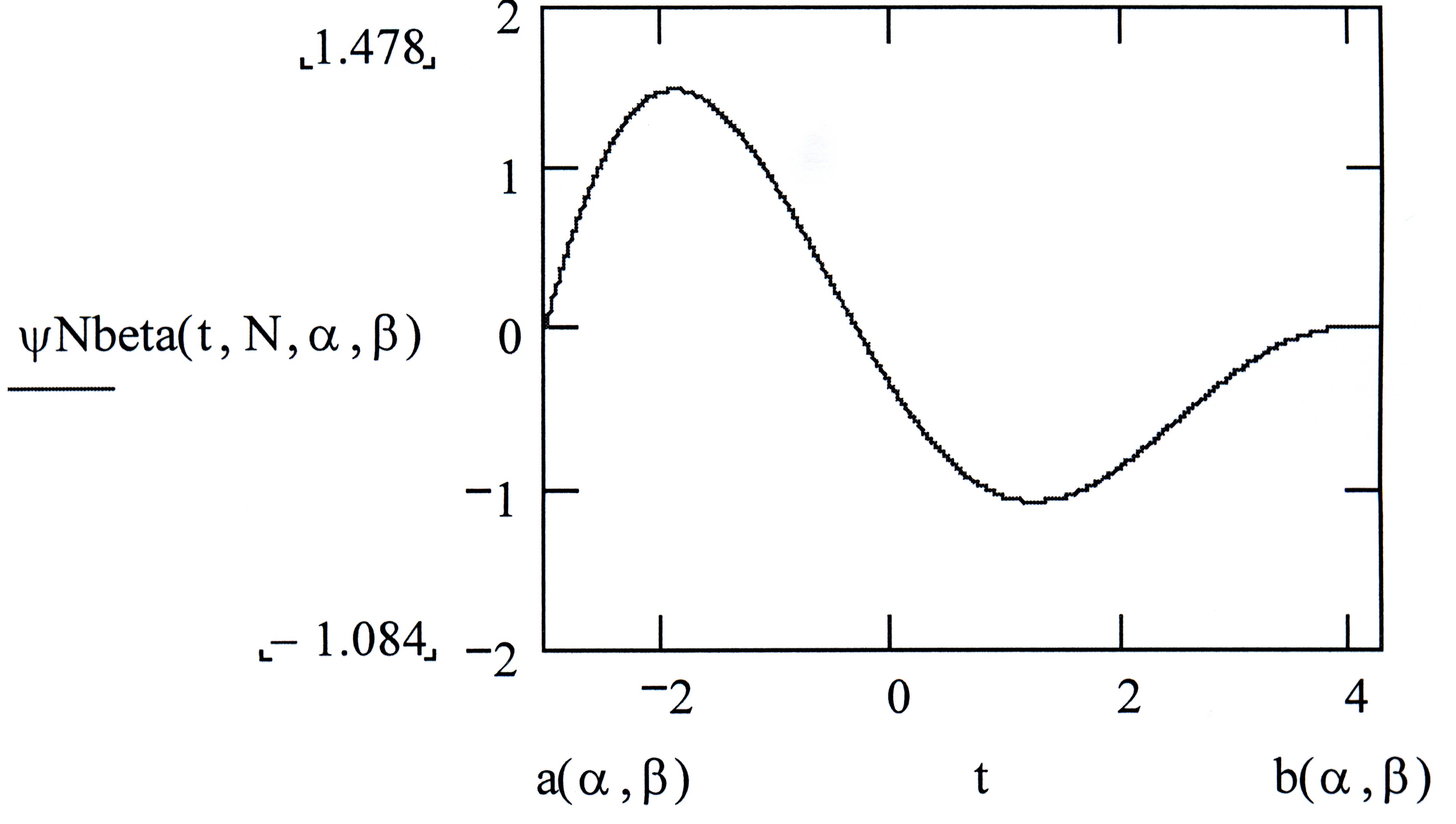
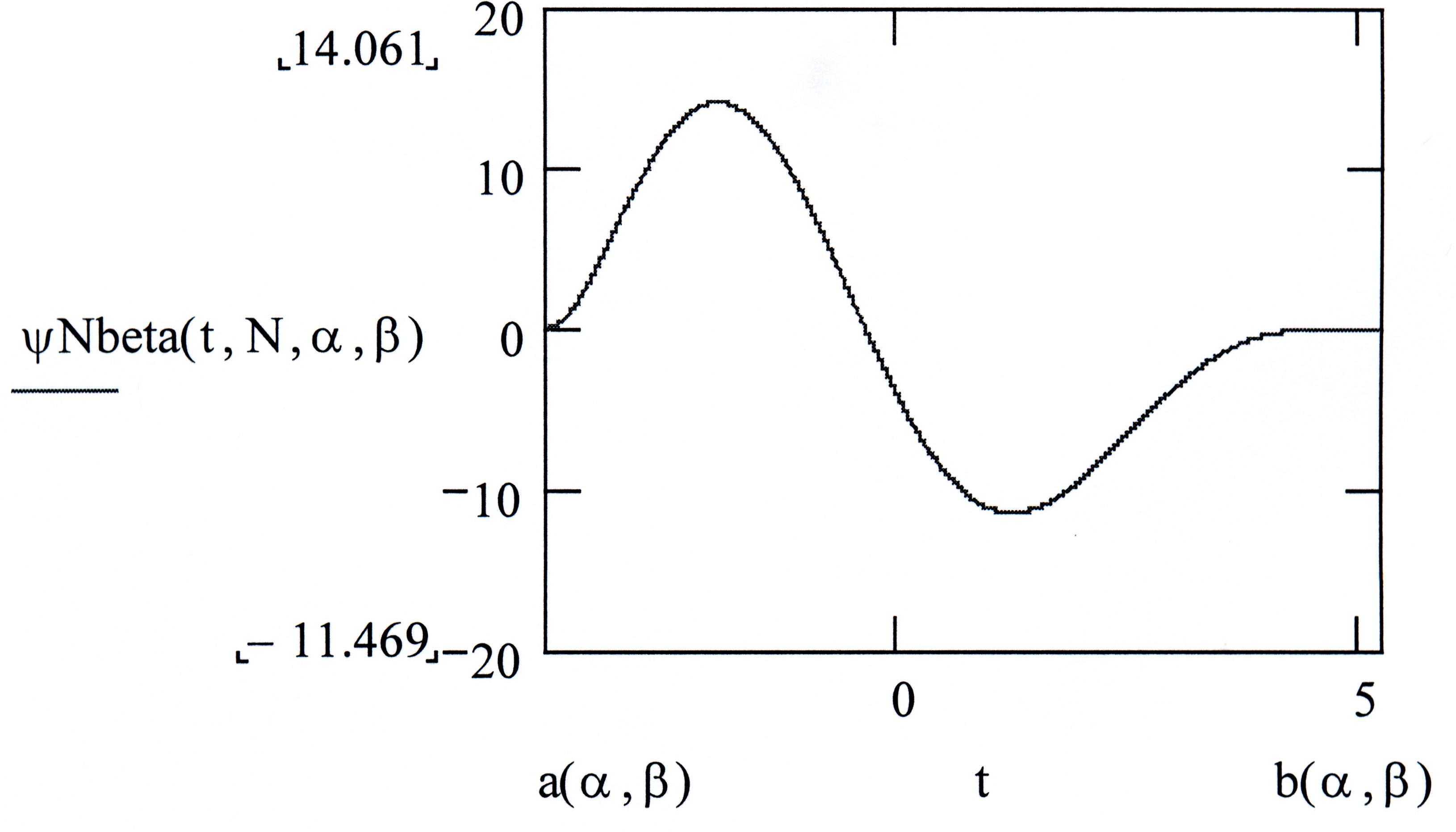
Figura 3: High-order beta wavelets for different parameters: a) $N=3$, $\alpha=5,\beta=7$; b) $N=5$, $\alpha=8,\beta=11$.

As it happens with any wavelet that has compact support, beta wavelets share the ability of providing good estimate for short transient, because no matter how short the interval is, there is a scaled wavelet version whose support is limited within this time. They can thus model local features efficiently as they are not concerned with the data behavior far way from the focused location. The main drawback of Haar wavelets is their discontinuities, which engender a broadband spectrum. In contrast, beta wavelets can provide a better balance between time and frequency resolution due to their soft shape. For a given support length (time resolution), a beta wavelet provides narrow spectrum (frequency resolution) than the corresponding Haar wavelet of the same support. Nowadays one of the most powerful software supporting wavelet analysis is the $Matlab^{TM}$ [16], especially when the wavelet graphic interface is available. In the $Matlab^{TM}$ wavelet toolbox, there exist five kinds of wavelets (type the command $waveinfo$ on the prompt): (i) crude wavelets, (ii) infinitely regular wavelets, (iii) orthogonal and compactly supported wavelets, (iv) biorthogonal and compactly supported wavelet pairs, (v) complex wavelets. Figure 4 illustrates the beta wavelet implementation over Matlab™. The m-files that allow the computation of the beta wavelet transform are currently $(freeware)$ available at the URL: http://www2.ee.ufpe.br/codec/WEBLET.html (new wavelets).

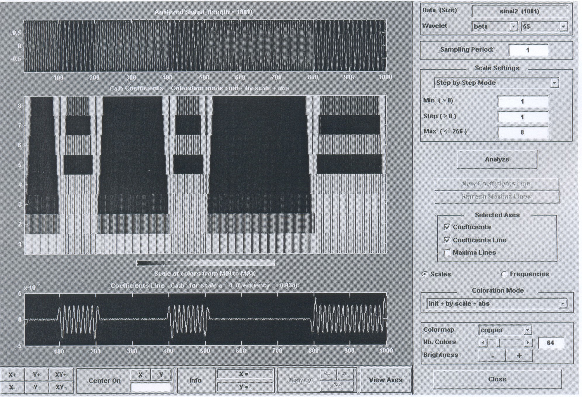
Figura 4: Beta wavelets displayed over $Matlab^{TM}$ using the wavemenu command. The analyzed signal is a binary FSK signal. This wavelet decomposition can be used to implement an efficient frequency discriminator.

IV CONCLUDING REMARKS

Compactly supported wavelets are among the most functional and useful wavelets. This correspondence introduces a new family of wavelets of this class. These wavelets can be viewed as some kind of soft-Haar wavelets. This new family of wavelets looks like a sort of soft-Haar wavelets, since both are unicycle wavelets. Besides the fact that beta wavelets are smoother, they have extra flexibility since the balance between the two half-cycles can be fine-tuned. However, it should be kept on mind that such a comparison is rather loose, since completeness and orthogonality properties that Haar wavelet holds were not addressed for beta wavelets. It remains to be investigated how beta wavelets can be approximated using FIR or IIR filters. In comparison with other wavelets of compact support (e.g. dBN, coiflets etc.), the beta wavelets derived in this work have idiosyncrasies and advantages: i) They are regular and smooth, ii) have only one cycle, iii) have an analytical formulation (close formulae), iv) Their importance rely on the Central Limit Theorem. Many practical signals have a cyclic true nature, that is, they are composed by uninterrupted cycles, as it occurs with power line signals, some biomedical signals or FSK signals. Since many waveforms are inborn-generated by successive cycles, their local properties can probably better investigated via a wavelet able to cope the changes from one cycle to another. It is often crucial to detect a small discrepancy within a cycle. This behavior can be useful for analyzing signals from certain modulation schemes or from power systems disturbances. Particularly, Beta-wavelet-based FSK modulation schemes are currently on investigation.

V ACKNOWLEDGMENTS

The authors thank Dr. Renato José de Sobral Cintra for quite a lot of comments, particularly regarding repeated convolution and Central Limit Theorems.

Lemma 1

The square of a normalized beta density

$$P(t)=\phi(t|\alpha,\beta)=\frac{1}{B(\alpha,\beta)}\cdot t^{\alpha-1}(1-t)^{\beta-1}$$ (46)

is proportional to another beta density.

Proof:

A straightforward algebraic handling yields $\phi^{2}(t|\alpha,\beta)=\lambda_{0}\cdot\phi(t|2\alpha-1,2\beta-1)$, where

$$\lambda_{0}=\lambda_{0}(\alpha,\beta)=\frac{B(2\alpha-1,2\beta-1)}{B^{2}(\alpha,\beta)}$$ (47)

∎

Let $D^{beta}=\{\phi_{beta}(t|\alpha,\beta)\}_{\alpha,\beta\in\mathbb{R}}$ be the set of all possible signals of the kind beta probability density (possibly non-normalized).

Lemma 2

The square of any beta density is proportional to another beta-shaped density of same support.

Proof:

The support of $\phi_{beta}(t|\alpha,\beta)$ remains unchanged and furthermore, $\phi^{2}_{beta}(t|\alpha,\beta)=\lambda\phi(t|2\alpha-1,2\beta-1),\quad t\in[a,b]$, where

$$\lambda_{0}=\lambda_{0}(\alpha,\beta) = {\frac{T(2\alpha-1,2\beta-1)^{2(\alpha+\beta-1)}}{T^{2}(\alpha,\beta)\cdot T(2\alpha-1,2\beta-1)}}.$$ (48)

∎

Corollary 1

$D^{beta}$ is a closed class of signals regarding the following operations: rising to a power (pair exponent) and repeated convolution (a number pair of times), i.e. $\phi_{beta}(t|\alpha,\beta)\in D^{beta}\Rightarrow\phi^{2}_{beta}(t|\alpha,\beta)\in D^{beta}$ and $\phi_{beta}(t|\alpha,\beta)\ast\phi_{beta}(t|\alpha,\beta)\in D^{beta}$.

A similar property is shared with the other densities concerned with versions of the Central Limit Theorem.

Lemma 3

$\frac{1}{2\pi}\int^{\infty}_{-\infty}|M(\alpha,\alpha+\beta,j\nu)|^{2}d\nu=\lambda_{0}(\alpha,\beta).$

Proof:

Parseval’s identity furnishes

$$\frac{1}{2\pi}\int^{\infty}_{-\infty}|M(\alpha,\alpha+\beta,j\nu)|^{2}d\nu=\int^{1}_{0}\phi_{beta}^{2}(t|\alpha,\beta)dt$$ (49)

and the proof follows by applying lemma 1. ∎

Lemma 4

The second moment of the square of the Kummer hypergeometric function $M(\alpha,\alpha+\beta,j\nu)$ is given by

$$\frac{1}{2\pi}\int^{\infty}_{-\infty}\nu^{2}|M(\alpha,\alpha+\beta,j\nu)|^{2}d\nu=\chi(\alpha,\beta),$$ (50)

where

$$\chi(\alpha,\beta) = \Bigl{(}\frac{1}{B^{2}(\alpha,\beta)}\Bigl{)}\Bigl{[}(\alpha-1)^{2}B(2\alpha-3,2\beta-3)$$ (51)

$$-2(\alpha-1)(\alpha+\beta-2)B(2\alpha-3,2\beta-3)$$

$$+(\alpha+\beta-2)^{2}B(2\alpha-3,2\beta-3)\Bigl{]}.$$

Proof:

It follows from Parseval’s identity that

$$\frac{1}{2\pi}\int^{\infty}_{-\infty}|\nu M(\alpha,\alpha+\beta,j\nu)|^{2}d\nu=\int^{1}_{0}\Bigl{[}\frac{d\phi(t|\alpha,\beta)}{dt}\Bigl{]}^{2}dt.$$ (52)

Now

$$\frac{d\phi(t|\alpha,\beta)}{dt}=\frac{1}{B(\alpha,\beta)}\cdot\Bigl{[}\frac{\alpha-1}{t}-\frac{\beta-1}{1-t}\Bigl{]}\cdot t^{\alpha-1}\cdot(1-t)^{\beta-1}$$ (53)

and therefore the evaluation of the integral

$$\int^{1}_{0}\Bigl{[}\frac{(\alpha-1)-(\alpha+\beta-2)\cdot t}{t(1-t)}\Bigl{]}^{2}\cdot t^{2\alpha-2}\cdot(1-t)^{2\beta-2}dt$$ (54)

completes the proof. ∎

The energy of the beta scale $\phi_{beta}(t|\alpha,\beta)$ and wavelet function $\psi_{beta}(t|\alpha,\beta)$ can be computed according to the following proposition.

Proposition 2

The energies of the beta scale and wavelet function are, respectively,

$$E_{\phi_{beta}}=\int^{\infty}_{-\infty}\phi^{2}_{beta}(t|\alpha,\beta)dt=\frac{\lambda_{0}(\alpha,\beta)}{T(\alpha,\beta)}$$ (55)

and

$$E_{\psi_{beta}}=\int^{\infty}_{-\infty}\psi^{2}_{beta}(t|\alpha,\beta)dt=\frac{\chi(\alpha,\beta)}{T^{3}(\alpha,\beta)}.$$ (56)

Proof:

A simple variable change gives

$$E_{\phi_{beta}}=\int^{b}_{a}\phi^{2}_{beta}(t|\alpha,\beta)dt=\frac{1}{T(\alpha,\beta)}\int^{b}_{a}\phi^{2}(t|\alpha,\beta)dt$$ (57)

and the proof of the first part follows by applying lemma 1. Let $\mathfrak{F}$ denote the Fourier transform operator. Parseval’s identity can be used in order to evaluate $E_{\psi_{beta}}$:

$$\int^{b}_{a}\psi^{2}_{beta}(t|\alpha,\beta)dt=\frac{1}{2\pi}\int^{\infty}_{-\infty}\Bigl{|}\mathfrak{F}\Bigl{(}\frac{dP(t|\alpha,\beta)}{dt}\Bigl{)}\Bigl{|}^{2}d\omega,$$ (58)

so that

$$E_{\psi_{beta}}=\frac{1}{2\pi}\int^{\infty}_{-\infty}\Bigl{|}\omega\cdot M(\alpha,\alpha+\beta,-j\omega\cdot T(\alpha,\beta))\Bigl{|}^{2}d\omega.$$ (59)

By a suitable variable change $\nu=\omega\cdot T(\alpha,\beta)$,

$$E_{\psi_{beta}}=\frac{1}{2\pi T^{3}(\alpha,\beta)}\int^{\infty}_{-\infty}\nu^{2}\Bigl{|}M(\alpha,\alpha+\beta,j\nu)\Bigl{|}^{2}d\nu$$ (60)

and the proof follows from lemma 4. ∎

Proposition 3

Let $\alpha>1$ and $\beta>1$. The admissibility constant $c_{\Psi}$ of a unicyclic beta wavelet is

$$c_{\psi}(\alpha,\beta)=\frac{2\pi\lambda_{0}(\alpha,\beta)}{T(\alpha,\beta)}<+\infty$$ (61)

Proof:

Since that

$$c_{\psi}=\int^{\infty}_{-\infty}\frac{|\Psi_{BETA}(\omega)|^{2}}{|\omega|}d\omega,$$ (62)

then

$$c_{\Psi}(\alpha,\beta)=\int^{\infty}_{-\infty}\Bigl{|}\omega M(\alpha,\alpha+\beta,-j\omega\cdot T(\alpha,\beta))\Bigl{|}^{2}d\omega$$ (63)

the proof is completed using the lemma 3. ∎

Further interesting properties of beta distributions can be found in [17].