Learning Parametric-Output HMMs with Two Aliased States

Abstract

In various applications involving hidden Markov models (HMMs), some of the hidden states are aliased, having identical output distributions. The minimality, identifiability and learnability of such aliased HMMs have been long standing problems, with only partial solutions provided thus far. In this paper we focus on parametric-output HMMs, whose output distributions come from a parametric family, and that have exactly two aliased states. For this class, we present a complete characterization of their minimality and identifiability. Furthermore, for a large family of parametric output distributions, we derive computationally efficient and statistically consistent algorithms to detect the presence of aliasing and learn the aliased HMM transition and emission parameters. We illustrate our theoretical analysis by several simulations.

1 Introduction

HMMs are a fundamental tool in the analysis of time series. A discrete time HMM with $n$ hidden states is characterized by a $n\times n$ transition matrix, and by the emissions probabilities from these $n$ states. In several applications, the HMMs, or more general processes such as partially observable Markov decision processes, are aliased, with some states having identical output distributions. In modeling of ion channel gating, for example, one postulates that at any given time an ion channel can be in only one of a finite number of hidden states, some of which are open and conducting current while others are closed, see e.g. Fredkin & Rice (1992). Given electric current measurements, one fits an aliased HMM and infers important biological insight regarding the gating process. Other examples appear in the fields of reinforcement learning (Chrisman, 1992; McCallum, 1995; Brafman & Shani, 2004; Shani et al., 2005) and robot navigation (Jefferies & Yeap, 2008; Zatuchna & Bagnall, 2009). In the latter case, aliasing occurs whenever different spatial locations appear (statistically) identical to the robot, given its limited sensing devices. As a last example, HMMs with several silent states that do not emit any output (Leggetter & Woodland, 1994; Stanke & Waack, 2003; Brejova et al., 2007), can also be viewed as aliased.

Key notions related to the study of HMMs, be them aliased or not, are their minimality, identifiability and learnability:

• Minimality. Is there an HMM with fewer states that induces the same distribution over all output sequences?

• Identifiability. Does the distribution over all output sequences uniquely determines the HMM’s parameters, up to a permutation of its hidden states?

• Learning. Given a long output sequence from a minimal and identifiable HMM, efficiently learn its parameters.

For non-aliased HMMs, these notions have been intensively studied and by now are relatively well understood, see for example Petrie (1969); Finesso (1990); Leroux (1992); Allman et al. (2009) and Cappé et al. (2005). The most common approach to learn the parameters of an HMM is via the Baum-Welch iterative algorithm (Baum et al., 1970). Recently, tensor decompositions and other computationally efficient spectral methods have been developed to learn non-aliased HMMs (Hsu et al., 2009; Siddiqi et al., 2010; Anandkumar et al., 2012; Kontorovich et al., 2013).

In contrast, the minimality, identifiability and learnability of aliased HMMs have been long standing problems, with only partial solutions provided thus far. For example, Blackwell & Koopmans (1957) characterized the identifiability of a specific aliased HMM with 4 states. The identifiability of deterministic output HMMs, where each hidden state outputs a deterministic symbol, was partially resolved by Ito et al. (1992). To the best of our knowledge, precise characterizations of the minimality, identifiability and learnability of probabilistic output HMMs with aliased states are still open problems. In particular, the recently developed tensor and spectral methods mentioned above, explicitly require the HMM to be non-aliasing, and are not directly applicable to learning aliased HMMs.

Main results.

In this paper we study the minimality, identifiability and learnability of parametric-output HMMs that have exactly two aliased states. This is the simplest possible class of aliased HMMs, and as shown below, even its analysis is far from trivial. Our main contributions are as follows: First, we provide a complete characterization of their minimality and identifiability, deriving necessary and sufficient conditions for each of these notions to hold. Our identifiability conditions are easy to check for any given 2-aliased HMM, and extend those of Ito et al. (1992) for the case of deterministic outputs. Second, we solve the problem of learning a possibly aliased HMM, from a long sequence of its outputs. To this end, we first derive an algorithm to detect whether an observed output sequence corresponds to a non-aliased HMM or to an aliased one. In the former case, the HMM  can be learned by various methods, such as Anandkumar et al. (2012); Kontorovich et al. (2013). In the latter case we show how the aliased states can be identified and present a method to recover the HMM parameters. Our approach is applicable to any family of output distributions whose mixtures are efficiently learnable. Examples include high dimensional Gaussians and products distributions, see Feldman et al. (2008); Belkin & Sinha (2010); Anandkumar et al. (2012) and references therein. After learning the output mixture parameters, our moment-based algorithm requires only a single pass over the data. It is possibly the first statistically consistent and computationally efficient scheme to handle 2-aliased HMMs. While our approach may be extended to more complicated aliasing, such cases are beyond the scope of this paper. We conclude with some simulations illustrating the performance of our suggested algorithms.

2 Definitions & Problem Setup

Notation.

We denote by $I_{n}$ the $n\times n$ identity matrix and $\boldsymbol{1}_{n}=(1,\dots,1)^{\textrm{\tiny{T}}}\in\mathbb{R}^{n}.$ For $\boldsymbol{v}\in\mathbb{R}^{n}$, $\operatorname{diag}(\boldsymbol{v})$ is the $n\times n$ diagonal matrix with entries $v_{i}$ on its diagonal. The $i$-th row and column of a matrix $A\in\mathbb{R}^{n\times n}$ are denoted by $A_{[i,\cdot]}$ and $A_{[\cdot,i]}$, respectively. We also denote $[n]=\{1,2,\dots,n\}$. For a discrete random variable $X$ we abbreviate $P(x)$ for $\Pr(X\!=\!x).$ For a second random variable $Z$, the quantity $P(z\,|\,x)$ denotes either $\Pr(Z=z\,|\,X=x)$, or the conditional density $p(Z=z|X=x),$ depending on whether $Z$ is discrete or continuous.

Hidden Markov Models.

Consider a discrete-time HMM with $n$ hidden states $\{1,\dots,n\}$, whose output alphabet $\mathcal{Y}$ is either discrete or continuous. Let $\mathcal{F}_{\theta}=\{f_{\theta}:\mathcal{Y}\to\mathbb{R}\,|\,\theta\in\Theta\}$ be a family of parametric probability density functions where $\Theta$ is a suitable parameter space. A parametric-output HMM is defined by a tuple $H=(A,\boldsymbol{\theta},\boldsymbol{\pi}^{0})$ where $A$ is the $n\times n$ transition matrix of the hidden states

$$A_{ij}=\Pr(X_{t+1}=i\,|\,X_{t}=j)=P(i\,|\,j),$$

$\boldsymbol{\pi}^{0}\in\mathbb{R}^{n}$ is the distribution of the initial state, and the vector of parameters $\boldsymbol{\theta}=(\theta_{1},\theta_{2},\dots,\theta_{n})\in\Theta^{n}$ determines the $n$ probability density functions $(f_{\theta_{1}},f_{\theta_{2}},\dots,f_{\theta_{n}})$.

The output sequence of the HMM is generated as follows. First, an unobserved Markov sequence of hidden states $x=(x_{t})_{t=0}^{T-1}$ is generated according to the distribution

$$P(x)=\pi^{0}_{x_{0}}\prod_{t=1}^{T-1}P(x_{t}\,|\,x_{t-1}).$$

The output $y_{t}\in\mathcal{Y}$ at time $t$ depends only on the hidden state $x_{t}$ via $P(y_{t}\,|\,x_{t})\equiv f_{\theta_{x_{t}}}(y_{t})$. Hence the conditional distribution of an output sequence $y=(y_{t})_{t=0}^{T-1}$ is

$$P(y\,|\,x)=\prod_{t=0}^{T-1}P(y_{t}\,|\,x_{t})=\prod_{t=0}^{T-1}f_{\theta_{x_{t}}}(y_{t}).$$

We denote by $P_{H,k}:\mathcal{Y}^{k}\to\mathbb{R}$ the joint distribution of the first $k$ consecutive outputs of the HMM $H$. For $y=(y_{0},\dots,y_{k-1})\in\mathcal{Y}^{k}$ this distribution is given by

$$P_{H,k}(y)=\sum_{x\in[n]^{k}}P(y\,|\,x)P(x).$$

Further we denote by $\mathcal{P}_{H}=\left\{P_{H,k}\,|\,k\geq 1\right\}$ the set of all these distributions.

2-Aliased HMMs.

For an HMM $H$ with output parameters $\boldsymbol{\theta}=(\theta_{1},\theta_{2},\dots,\theta_{n})\in\Theta^{n}$ we say that states $i$ and $j$ are aliased if $\theta_{i}=\theta_{j}$. In this paper we consider the special case where $H$ has exactly two aliased states, denoted as 2A-HMM. Without loss of generality, we assume the aliased states are the two last ones, $n\!-\!1$ and $n$. Thus,

$$\theta_{1}\neq\theta_{2}\neq\dots\neq\theta_{n-2}\neq\theta_{n\!-\!1}\quad\text{and}\quad\theta_{n-1}=\theta_{n}.$$

We denote the vector of the $n\!-\!1$ unique output parameters of $H$ by $\bar{\boldsymbol{\theta}}=(\theta_{1},\theta_{2},\dots,\theta_{n-2},\theta_{n\!-\!1})\in\Theta^{n-1}.$ For future use, we define the aliased kernel ${\bar{K}}\in\mathbb{R}^{(n\!-\!1)\times(n\!-\!1)}$ as the matrix of inner products between the $n\!-\!1$ different $f_{\theta_{i}}$’s,

$${\bar{K}}_{ij}\equiv\langle f_{\theta_{i}},f_{\theta_{j}}\rangle=\int_{\mathcal{Y}}f_{\theta_{i}}(y)f_{\theta_{j}}(y)\textrm{d}y,\quad i,j\in[n\!-\!1].$$ (1)

Assumptions.

As in previous works (Leroux, 1992; Kontorovich et al., 2013), we make the following standard assumptions:

• The parametric family $\mathcal{F}_{\theta}$ of the output distributions is linearly independent of order $n$: for any distinct $\{\theta_{i}\}_{i=1}^{n}$, $\sum_{i=1}^{n}a_{i}f_{\theta_{i}}\equiv 0$ iff $a_{i}=0$ for all $i\in[n].$

• The transition matrix $A$ is ergodic and its unique stationary distribution $\boldsymbol{\pi}=(\pi_{1},\pi_{2},\dots,\pi_{n})$ is positive.

Note that assumption (A1) implies that the parametric family $\mathcal{F}_{\theta}$ is identifiable, namely $f_{\theta}=f_{\theta^{\prime}}$ iff $\theta=\theta^{\prime}$. It also implies that the kernel matrix ${\bar{K}}$ of (1) is full rank $n\!-\!1$.

3 Decomposing the transition matrix $A$

The main tool in our analysis is a novel decomposition of the 2A-HMM’s transition matrix into its non-aliased and aliased parts. As shown in Lemma 1 below, the aliased part consists of three rank-one matrices, that correspond to the dynamics of exit from, entrance to, and within the two aliased states. This decomposition is used to derive the conditions for minimality and identifiability (Section 4), and plays a key role in learning the HMM (Section 5).

To this end, we introduce a pseudo-state $\bar{n}$, combining the two aliased states $n\!-\!1$ and $n$. We define

$$\pi_{\bar{n}}=\pi_{n-1}+\pi_{n}\quad\mbox{and}\quad\beta={\pi_{n-1}}/{\pi_{\bar{n}}}.$$ (2)

We shall make extensive use of the following two matrices:

$$B = \left(\begin{array}[]{ccc|cc}&&&0&0\\[-5.0pt] &I_{n-2}&&\vdots&\vdots\\ &&&0&0\\ \hline\cr 0&\dots&0&1&1\\ \end{array}\right)\in\mathbb{R}^{(n\!-\!1)\times n},$$

$$C_{\beta} = \left(\begin{array}[]{ccc|c}&&&0\\[-5.0pt] &I_{n-2}&&\vdots\\ &&&0\\ \hline\cr 0&\dots&0&\beta\\ 0&\dots&0&1\!-\!\beta\\ \end{array}\right)\in\mathbb{R}^{n\times(n\!-\!1)}.$$

As explained below, these matrices can be viewed as projection and lifting operators, mapping between non-aliased and aliased quantities.

Non-aliased part.

The non-aliased part of $A$ is a stochastic matrix $\bar{A}\in\mathbb{R}^{(n\!-\!1)\times(n\!-\!1)}$, obtained by merging the two aliased states $n\!-\!1$ and $n$ into the pseudo-state $\bar{n}$. Its entries are given by

$$\bar{A}\!=\!\left(\begin{array}[]{ccc|c}&&&P(1\,|\,\bar{n})\\ &A_{[1:n\!-\!2]\times[1:n\!-\!2]}&&\vdots\\ &&&P(n\!-\!2\,|\,\bar{n})\\[3.0pt] \hline\cr\rule[11.0pt]{0.0pt}{0.0pt}P(\bar{n}\,|\,1)&\dots&P(\bar{n}\,|\,n\!-\!2)&P(\bar{n}\,|\,\bar{n})\end{array}\right),$$ (9)

where the transition probabilities into the pseudo-state are

$$P(\bar{n}\,|\,j) = P(n\!-\!1\,|\,j)+P(n\,|\,j),\quad\forall j\in[n],$$

the transition probabilities out of the pseudo-state are defined with respect to the stationary distribution by

$$P(i\,|\,\bar{n}) = \beta P(i\,|\,n\!-\!1)+(1\!-\!\beta)P(i\,|\,n),\quad\forall i\in[n]$$

and lastly, the probability to stay in the pseudo-state is

$$P(\bar{n}\,|\,\bar{n}) = \beta P(\bar{n}\,|\,n\!-\!1)+(1\!-\!\beta)P(\bar{n}\,|\,n).$$

It is easy to check that the unique stationary distribution of $\bar{A}$ is $\bar{\boldsymbol{\pi}}=(\pi_{1},\pi_{2},\dots,\pi_{n\!-\!2},\pi_{\bar{n}})\in\mathbb{R}^{n\!-\!1}$. Finally, note that $\bar{A}=BAC_{\beta}$, $\bar{\boldsymbol{\pi}}=B\boldsymbol{\pi}$ and $\boldsymbol{\pi}=C_{\beta}\bar{\boldsymbol{\pi}}$, justifying the lifting and projection interpretation of the matrices $B,C_{\beta}$.

Aliased part.

Next we present some key quantities that distinguish between the two aliased states. Let $\operatorname{supp}_{{\textrm{\tiny{in}}}}=\{j\in[n]\,|\,P(\bar{n}\,|\,j)>0\}$ be the set of states that can move into either one of the aliased states. We define

$$\alpha_{j} = \begin{cases}\frac{P(n\!-\!1\,|\,j)}{P(\bar{n}\,|\,j)}&j\in\operatorname{supp}_{{\textrm{\tiny{in}}}}\\ 0&\text{otherwise},\end{cases}$$ (10)

as the relative probability of moving from state $j$ to state $n\!-\!1$, conditional on moving to either $n\!-\!1$ or $n$. We define the two vectors ${{\boldsymbol{\delta}}^{\operatorname{out}}},{{\boldsymbol{\delta}}^{\operatorname{in}}}\in\mathbb{R}^{n-1}$ as follows: $\forall i,j\in[n\!-\!1]$,

$${\delta}^{\operatorname{out}}_{i} = \begin{cases}P(i\,|\,n\!-\!1)-P(i\,|\,n)&i<n-1\\ P(\bar{n}\,|\,n\!-\!1)-P(\bar{n}\,|\,n)&i=n-1\end{cases}$$ (11)

$${\delta}^{\operatorname{in}}_{j} = \begin{cases}(\alpha_{j}\!-\!\beta)P(\bar{n}\,|\,j)&j<n\!-\!1\\[5.0pt] \beta(\alpha_{n\!-\!1}\!-\!\beta)P(\bar{n}\,|\,n\!-\!1)\\ \quad+\,(1\!-\!\beta)(\alpha_{n}\!-\!\beta)P(\bar{n}\,|\,n)&j=n\!-\!1.\end{cases}$$ (12)

In other words, ${{\boldsymbol{\delta}}^{\operatorname{out}}}$ captures the differences in the transition probabilities out of the aliased states. In particular, if ${{\boldsymbol{\delta}}^{\operatorname{out}}}=\boldsymbol{0}$ then starting from either one of the two aliased states, the Markov chain evolution is identical. Intuitively such an HMM is not minimal, as its two aliased states can be lumped together, see Theorem 1 below.

Similarly, ${{\boldsymbol{\delta}}^{\operatorname{in}}}$ compares the relative probabilities into the aliased states $\alpha_{j}$, to the stationary relative probability $\beta={\pi_{n-1}}/{\pi_{\bar{n}}}$. This quantity also plays a role in the minimality of the HMM.

Lastly, for our decomposition, we define the scalar

$$\kappa=(\alpha_{n\!-\!1}-\beta)P(\bar{n}\,|\,n\!-\!1)-(\alpha_{n}-\beta)P(\bar{n}\,|\,n).$$ (13)

Decomposing $A$.

The following lemma provides a decomposition of the transition matrix in terms of $\bar{A}$, ${{\boldsymbol{\delta}}^{\operatorname{out}}}$, ${{\boldsymbol{\delta}}^{\operatorname{in}}}$, $\kappa$ and $\beta$ (all omitted proofs are given in the Appendix).

Lemma 1.

The transition matrix $A$ of a 2A-HMM can be written as

$$A=C_{\beta}\bar{A}B+C_{\beta}{{\boldsymbol{\delta}}^{\operatorname{out}}}\boldsymbol{c}_{\beta}^{\textrm{\tiny{T}}}+\boldsymbol{b}({{\boldsymbol{\delta}}^{\operatorname{in}}})^{{\textrm{\tiny{T}}}}B+\kappa\,\boldsymbol{b}\boldsymbol{c}_{\beta}^{\textrm{\tiny{T}}},$$ (14)

where ${\boldsymbol{c}_{\beta}}^{{\textrm{\tiny{T}}}}=(0,\dots,0,{1\!-\!\beta},-\beta)\in\mathbb{R}^{n}$ and $\boldsymbol{b}=(0,\dots,0,1,-1)^{{\textrm{\tiny{T}}}}\in\mathbb{R}^{n}.$

In (14), the first term is the merged transition matrix $\bar{A}\in\mathbb{R}^{(n\!-\!1)\times(n\!-\!1)}$ lifted back into $\mathbb{R}^{n\times n}$. This term captures all of the non-aliased transitions. The second matrix is zero except in the last two columns, accounting for the exit transition probabilities from the two aliased states. Similarly, the third matrix is zero except in the last two rows, differentiating the entry probabilities. The fourth term is non-zero only on the lower right $2\times 2$ block involving the aliased states $n\!-\!1$, $n$. This term corresponds to the internal dynamics between them. Note that each of the last three terms is at most a rank-$1$ matrix, which together can be seen as a perturbation due to the presence of aliasing.

In section 5 we shall see that given a long output sequence from the HMM, the presence of aliasing can be detected and the quantities $\bar{A}$, ${{\boldsymbol{\delta}}^{\operatorname{out}}}$, ${{\boldsymbol{\delta}}^{\operatorname{in}}}$, $\kappa$ and $\beta$ can all be estimated from it. An estimate for $A$ is then obtained via Eq. (14).

4 Minimality and Identifiability

Two HMMs $H$ and $H^{\prime}$ are said to be equivalent if their observed output sequences are statistically indistinguishable, namely $\mathcal{P}_{H^{\prime}}=\mathcal{P}_{H}$. Similarly, an HMM $H$ is minimal if there is no equivalent HMM with fewer number of states. Note that if $H$ is non-aliased then Assumptions (A1-A2) readily imply that it is also minimal (Leroux, 1992). In this section we present necessary and sufficient conditions for a 2A-HMM to be minimal, and for two minimal 2A-HMMs to be equivalent. Finally, we derive necessary and sufficient conditions for a minimal 2A-HMM to be identifiable.

4.1 Minimality

The minimality of an HMM is closely related to the notion of lumpability: can hidden states be merged without affecting the distribution $\mathcal{P}_{H}$ (Fredkin & Rice, 1986; White et al., 2000; Huang et al., 2014). Obviously, an HMM is minimal iff no subset of hidden states can be merged. In the following theorem we give precise conditions for the minimality of a 2A-HMM.

Theorem 1.

Let $H$ be a 2A-HMM satisfying Assumptions (A1-A2) whose initial state $X_{0}$ is distributed according to $\boldsymbol{\pi}^{0}=(\pi^{0}_{1},\pi^{0}_{2},\dots,\beta^{0}\pi^{0}_{\bar{n}},(1\!-\!\beta^{0})\pi^{0}_{\bar{n}}).$ Then,

• If $\pi^{0}_{\bar{n}}\neq 0$ and $\beta^{0}\neq\beta$ then $H$ is minimal iff ${{\boldsymbol{\delta}}^{\operatorname{out}}}\neq\boldsymbol{0}$.

• If $\pi^{0}_{\bar{n}}=0$ or $\beta^{0}=\beta$ then $H$ is minimal iff both ${{\boldsymbol{\delta}}^{\operatorname{out}}}\neq~{}\boldsymbol{0}$ and ${{\boldsymbol{\delta}}^{\operatorname{in}}}\neq\,\boldsymbol{0}$.

By Theorem 1, a necessary condition for minimality of a 2A-HMM is that the two aliased states have different exit probabilities, ${{\boldsymbol{\delta}}^{\operatorname{out}}}\neq 0$. Namely, there exists a non-aliased state $i\in[n\!-\!2]$ such that $P(i\,|\,n\!-\!1)\neq P(i\,|\,n)$. Otherwise the two aliased states can be merged. If the 2A-HMM is started from its stationary distribution, then an additional necessary condition is ${{\boldsymbol{\delta}}^{\operatorname{in}}}\neq 0$. This last condition implies that there is a non-aliased state $j\in\operatorname{supp}_{{\textrm{\tiny{in}}}}\setminus\{n\!-\!1,n\}$ with relative entrance probability $\alpha_{j}\neq\beta$.

4.2 Identifiability

Recall that an HMM $H$ is (strictly) identifiable if $\mathcal{P}_{H}$ uniquely determines the transition matrix $A$ and the output parameters $\boldsymbol{\theta}$, up to a permutation of the hidden states. We establish the conditions for identifiability of a 2A-HMM in two steps. First we derive a novel geometric characterization of the set of all minimal HMMs that are equivalent to $H$, up to a permutation of the hidden states (Theorem 2). Then we give necessary and sufficient conditions for $H$ to be identifiable, namely for this set to be the singleton set, consisting of only $H$ itself (Appendix C). In the process, we provide a simple procedure (Algorithm 1) to determine whether a given minimal 2A-HMM is identifiable or not.

Equivalence between minimal 2A-HMMs.

Necessary and sufficient conditions for the equivalence of two minimal HMMs were studied in several works (Finesso, 1990; Ito et al., 1992; Vanluyten et al., 2008). We now provide analogous conditions for parametric output 2A-HMMs. Toward this end, we define the following 2-dimensional family of matrices $S(\tau_{n-1},\tau_{n})\in\mathbb{R}^{n\times n}$ given by

$$S(\tau_{n-1},\tau_{n})=\left(\begin{array}[]{ccc|cc}&&&0&0\\[-4.0pt] &I_{n-2}&&\vdots&\vdots\\ &&&0&0\\ \hline\cr 0&\dots&0&\tau_{n\!-\!1}&\tau_{n}\\ 0&\dots&0&1\!-\!\tau_{n\!-\!1}&1\!-\!\tau_{n}\end{array}\right).$$

Clearly, for $\tau_{n\!-\!1}\neq\tau_{n}$, $S$ is invertible. As in Ito et al. (1992), consider then the following similarity transformation of the transition matrix $A,$

$$A_{H}(\tau_{n-1},\tau_{n}) \!\!=\!\! S(\tau_{n-1},\tau_{n})^{-1}AS(\tau_{n-1},\tau_{n}).$$ (16)

It is easy to verify that $\boldsymbol{1}^{\textrm{\tiny{T}}}_{n}A_{H}=\boldsymbol{1}^{\textrm{\tiny{T}}}_{n}$. However, $A_{H}$ is not necessarily stochastic, as depending on $\tau_{n-1},\tau_{n}$ it may have negative entries. The following lemma resolves the equivalence of 2A-HMMs, in terms of this transformation.

Lemma 2.

Let $H=(A,\boldsymbol{\theta},\boldsymbol{\pi})$ be a minimal 2A-HMM satisfying Assumptions (A1-A2). Then a minimal HMM $H^{\prime}=(A^{\prime},\boldsymbol{\theta}^{\prime},\boldsymbol{\pi}^{\prime})$ with $n^{\prime}$ states is equivalent to $H$ iff $n^{\prime}=n$ and there exists a permutation matrix $\Pi\in\mathbb{R}^{n\times n}$ and $\tau_{n-1}>\tau_{n}$ such that $\boldsymbol{\theta}^{\prime}=\Pi\,\boldsymbol{\theta}$ and

$$\boldsymbol{\pi}^{\prime} = \Pi\,S(\tau_{n-1},\tau_{n})^{-1}\boldsymbol{\pi}$$

$$A^{\prime} = \Pi\,A_{H}(\tau_{n-1},\tau_{n})\,\Pi^{-1}\,\geq\,0.$$

The feasible region.

By Lemma 2, any matrix $A_{H}(\tau_{n-1},\tau_{n})$ whose entries are all non-negative yields an HMM equivalent to the original one. We thus define the feasible region of $H$ by

$$\Gamma_{H}=\{(\tau_{n\!-\!1},\tau_{n})\in\mathbb{R}^{2}\,|\,A_{H}(\tau_{n\!-\!1},\tau_{n})\geq 0,\,\tau_{n\!-\!1}\!>\!\tau_{n}\}.$$ (17)

By definition, $\Gamma_{H}$ is non-empty, since $(\tau_{n-1},\tau_{n})=(1,0)$ recover the original matrix $A$. As we show below, $\Gamma_{H}$ is determined by three simpler regions $\Gamma_{1},\Gamma_{2},\Gamma_{3}\subset\mathbb{R}^{2}$. The region $\Gamma_{1}$ ensures that all entries of $A_{H}$ are non-negative except possibly in the lower right $2\times 2$ block corresponding to the two aliased states. The regions $\Gamma_{2}$ and $\Gamma_{3}$ ensure non-negativity of the latter, depending on whether the aliased relative probabilities of (10) satisfy $\alpha_{n\!-\!1}\geq\alpha_{n}$ or $\alpha_{n\!-\!1}<\alpha_{n}$, respectively. For ease of exposition we assume as a convention that $P(\bar{n}\,|\,n\!-\!1)\geq P(\bar{n}\,|\,n)$.

Theorem 2.

Let $H$ be a minimal 2A-HMM satisfying Assumptions (A1-A2). There exist $(\tau^{\min}_{n\!-\!1},\tau^{\min}_{n})$, $(\tau^{\max}_{n\!-\!1},\tau^{\max}_{n})$, $(\tau^{-},\tau^{+})\in\mathbb{R}^{2}$, and convex monotonic decreasing functions $f,g:\mathbb{R}\to\mathbb{R}$ such that

$$\Gamma_{H}=\begin{cases}\Gamma_{1}\cap\Gamma_{2}&\alpha_{n\!-\!1}\geq\alpha_{n}\\ \Gamma_{1}\cap\Gamma_{3}&\alpha_{n\!-\!1}<\alpha_{n},\end{cases}$$

where the regions $\Gamma_{1},\Gamma_{2},\Gamma_{3}\subset\mathbb{R}^{2}$ are given by

$$\Gamma_{1} = [\tau^{\min}_{n\!-\!1},\tau^{\max}_{n\!-\!1}]\times[\tau^{\max}_{n},\tau^{\min}_{n}]$$

$$\Gamma_{2} = [\tau^{+},\infty)\times[\tau^{-},\tau^{+}]$$

$$\Gamma_{3} = \{(\tau_{n\!-\!1},\tau_{n})\in\Gamma_{1}\,|\,\,f(\tau_{n\!-\!1})\leq\tau_{n}\leq g(\tau_{n\!-\!1})\,\}.$$

In addition, the set $\Gamma_{H}$ is connected.

The feasible regions in the two possible cases ($\alpha_{n\!-\!1}\geq\alpha_{n}$ or $\alpha_{n\!-\!1}<\alpha_{n}$) are depicted in Appendix C, Fig.6.

Strict Identifiability.

By Lemma 2, for strict identifiability of $H$, ${\Gamma_{H}}$ should be the singleton set ${\Gamma_{H}}=\{(1,0)\}$. Due to lack of space, sufficient and necessary conditions for this to hold, as well as a corresponding simple procedure to determine whether a 2A-HMM is identifiable, are given in Appendix 8.

Remark. While beyond the scope of this paper, we note that instead of strict identifiability of a given HMM, several works studied a different concept of generic identifiability (Allman et al., 2009), proving that under mild conditions the class of HMMs is generically identifiable. In contrast, if we restrict ourselves to the class of 2A-HMMs, then our Theorem 2 implies that this class is generically non-identifiable. The reason is that by Theorem 2, for any 2A-HMM whose matrix $A$ has all its entries positive, there are an infinite number of equivalent 2A-HMMs, implying non-identifiability.

5 Learning a 2A-HMM

Let $(Y_{t})_{t=0}^{T-1}$ be an output sequence generated by a parametric-output HMM that satisfies Assumptions (A1-A2) and initialized with its stationary distribution, $X_{0}\sim\boldsymbol{\pi}$. We assume the HMM is either non-aliasing, with $n\!-\!1$ states, or 2-aliasing with $n$ states. We further assume that the HMM is minimal and identifiable, as otherwise its parameters cannot be uniquely determined.

In this section we study the problems of detecting whether the HMM is aliasing and recovering its output parameters $\boldsymbol{\theta}$ and transition matrix $A$, all in terms of $(Y_{t})_{t=0}^{T-1}$.

Figure 1: Learning a 2A-HMM.

High level description.

The proposed learning procedure consists of the following steps (see Fig.1):

• Determine the number of output components $n\!-\!1$ and estimate the $n\!-\!1$ unique output distribution parameters $\bar{\boldsymbol{\theta}}$ and the projected stationary distribution $\bar{\boldsymbol{\pi}}$.

• Detect if the HMM is 2-aliasing.

• In case of a non-aliased HMM, estimate the $(n\!-\!1)\times(n\!-\!1)$ transition matrix $\bar{A}$, as for example in Kontorovich et al. (2013) or Anandkumar et al. (2012).

• In case of a 2-aliased HMM, identify the component $\theta_{n\!-\!1}$ corresponding to the two aliased states, and estimate the $n\times n$ transition matrix $A$.

We now describe in detail each of these steps. As far as we know, our learning procedure is the first to consistently learn a 2A-HMM in a computationally efficient way. In particular, the solutions for problems (ii) and (iv) are new.

Estimating the output distribution parameters.

As the HMM is stationary, each observable $Y_{t}$ is a random realization from the following parametric mixture model,

$$Y\sim\sum_{i=1}^{n\!-\!1}\bar{\pi}_{i}f_{\bar{\theta}_{i}}(y).$$ (18)

Hence, the number of unique output components $n-1$, the corresponding output parameters $\bar{\boldsymbol{\theta}}$ and the projected stationary distribution $\bar{\boldsymbol{\pi}}$ can be estimated by fitting a mixture model (18) to the observed output sequence $(Y_{t})_{t=0}^{T-1}$.

Consistent methods to determine the number of components in a mixture are well known in the literature (Titterington et al., 1985). The estimation of $\bar{\boldsymbol{\theta}}$ and $\bar{\boldsymbol{\pi}}$ is typically done by either applying an EM algorithm, or any recently developed spectral method (Dasgupta, 1999; Achlioptas & McSherry, 2005; Anandkumar et al., 2012). As our focus is on the aliasing aspects of the HMM, in what follows we assume that the number of unique output components $n\!-\!1$, the output parameters $\bar{\boldsymbol{\theta}}$ and the projected stationary distribution $\bar{\boldsymbol{\pi}}$ are exactly known. As in Kontorovich et al. (2013), it is possible to show that our method is robust to small perturbations in these quantities (not presented).

5.1 Moments

To solve problems (ii), (iii) and (iv) above, we first introduce the moment-based quantities we shall make use of. Given $\bar{\boldsymbol{\theta}}$ and $\bar{\boldsymbol{\pi}}$ or estimates of them, for any $i,j\in[n\!-\!1]$, we define the second order moments with time lag $t$ by

$${\mathcal{M}}^{(t)}_{ij}=\text{{\bf E}}[f_{\theta_{i}}(Y_{0})f_{\theta_{j}}(Y_{t})],\quad t\in\{1,2,3\}.$$ (19)

The consecutive in time third order moments are defined by

$${\mathcal{G}}^{(c)}_{ij}=\text{{\bf E}}[f_{\theta_{i}}(Y_{0})f_{\theta_{c}}(Y_{1})f_{\theta_{j}}(Y_{2})],\quad\forall c\in[n\!-\!1].$$ (20)

We also define the lifted kernel, $\mathcal{K}=B^{{\textrm{\tiny{T}}}}{\bar{K}}B\in\mathbb{R}^{n\times n}.$ One can easily verify that for a 2A-HMM,

$${\mathcal{M}}^{(t)} = {\bar{K}}BA^{t}C_{\beta}\operatorname{diag}(\bar{\boldsymbol{\pi}}){\bar{K}}$$ (21)

$${\mathcal{G}}^{(c)} = {\bar{K}}BA\operatorname{diag}({\mathcal{K}}_{[\cdot,c]})AC_{\beta}\operatorname{diag}(\bar{\boldsymbol{\pi}}){\bar{K}}.$$ (22)

Next we define the kernel free moments ${M}^{(t)},{G}^{(c)}\in\mathbb{R}^{(n\!-\!1)\times(n\!-\!1)}$ as follows:

$${M}^{(t)} \!=\! {\bar{K}}^{-1}{\mathcal{M}}^{(t)}{\bar{K}}^{-1}\operatorname{diag}(\bar{\boldsymbol{\pi}})^{-1}$$ (23)

$${G}^{(c)} \!=\! {\bar{K}}^{-1}{\mathcal{G}}^{(c)}{\bar{K}}^{-1}\operatorname{diag}(\bar{\boldsymbol{\pi}})^{-1}.$$ (24)

Note that by Assumption (A1), the kernel ${\bar{K}}$ is full rank and thus ${\bar{K}}^{-1}$ exists. Similarly, by (A2) $\bar{\boldsymbol{\pi}}>0$, so $\operatorname{diag}(\bar{\boldsymbol{\pi}})^{-1}$ also exists. Thus, (23,24) are well defined.

Let $R^{(2)},R^{(3)},F^{(c)}\in\mathbb{R}^{(n\!-\!1)\times(n\!-\!1)}$ be given by

$$R^{(2)} ={M}^{(2)}-({M}^{(1)})^{2}$$ (25)

$$R^{(3)} ={M}^{(3)}\!-\!{M}^{(2)}{M}^{(1)}\!-\!{M}^{(1)}{M}^{(2)}+({M}^{(1)})^{3}$$ (26)

$$F^{(c)} ={G}^{(c)}-{M}^{(1)}\operatorname{diag}({\bar{K}}_{[\cdot,c]}){M}^{(1)}.$$ (27)

The following key lemma relates the moments (25, 26, 27) to the decomposition (14) of the transition matrix $A$.

Lemma 3.

Let $H$ be a minimal 2A-HMM with aliased states $n\!-\!1$ and $n$. Let $\bar{A}$, ${{\boldsymbol{\delta}}^{\operatorname{out}}}$, ${{\boldsymbol{\delta}}^{\operatorname{in}}}$ and $\kappa$ be defined in (9,11,12,13) respectively. Then the following relations hold:

$${M}^{(1)} = \bar{A}$$ (28)

$$R^{(2)} = {{\boldsymbol{\delta}}^{\operatorname{out}}}({{\boldsymbol{\delta}}^{\operatorname{in}}})^{\textrm{\tiny{T}}}$$ (29)

$$R^{(3)} = \kappa R^{(2)}$$ (30)

$$F^{(c)} = {\bar{K}}_{{n\!-\!1},c}R^{(2)},\quad\forall c\in[n\!-\!1].$$ (31)

In the following, these relations will be used to detect aliasing, identify the aliased states and recover the aliased transition matrix $A$.

Empirical moments.

In practice, the unknown moments (19,20) are estimated from the output sequence $(Y_{t})_{t=0}^{T-1}$ by

$${\hat{\mathcal{M}}}^{(t)}_{ij} = \frac{1}{T-t}\sum_{l=0}^{T-t-1}f_{\theta_{i}}(Y_{l})f_{\theta_{j}}(Y_{l+t}),$$

$${\hat{\mathcal{G}}}^{(c)}_{ij} = \frac{1}{T-2}\sum_{l=0}^{T-3}f_{\theta_{i}}(Y_{l})f_{\theta_{c}}(Y_{l+1})f_{\theta_{j}}(Y_{l+2}).$$

With ${\bar{K}},\bar{\boldsymbol{\pi}}$ known, the corresponding empirical kernel free moments are given by

$${\hat{M}}^{(t)} = {\bar{K}}^{-1}{\hat{\mathcal{M}}}^{(t)}{\bar{K}}^{-1}\operatorname{diag}(\bar{\boldsymbol{\pi}})^{-1}$$ (32)

$${\hat{G}}^{(c)} = {\bar{K}}^{-1}{\hat{\mathcal{G}}}^{(c)}{\bar{K}}^{-1}\operatorname{diag}(\bar{\boldsymbol{\pi}})^{-1}.$$ (33)

The empirical estimates for (25,26,27) similarly follow.

To analyze the error between the empirical and population quantities, we make the following additional assumption:

(A3) The output distributions are bounded. Namely there exists $L>0$ such that $\forall i\in[n]$ and $\forall y\in\mathcal{Y}$, $f_{\theta_{i}}(y)\leq L$.

Lemma 4.

Let $(Y_{t})_{t=0}^{T-1}$ be an output sequence generated by an HMM satisfying Assumptions (A1-A3). Then, as $T\to\infty$, for any $t\in\{1,2,3\}$ and $c\in[n\!-\!1]$, all error terms ${\hat{M}}^{(t)}-{M}^{(t)}$, $\hat{R}^{(t)}-R^{(t)}$ and $\hat{F}^{(c)}-F^{(c)}$ are $O_{P}(T^{-\frac{1}{2}})$.

In fact, due to strong mixing, all of the above quantities are asymptotically normally distributed (Bradley, 2005).

5.2 Detection of aliasing

We now proceed to detect if the HMM is aliased (step (ii) in Fig.1). We pose this as a hypothesis testing problem:

$$\begin{array}[]{l}\mathcal{H}_{0}:\,\text{$H$ is non-aliased with $n\!-\!1$ states}\\ \hskip 75.0pt\text{vs.}\\ \mathcal{H}_{1}:\,\text{$H$ is 2-aliased with $n$ states}.\end{array}$$

We begin with the following simple observation:

Lemma 5.

Let $H$ be a minimal non-aliased HMM with $n\!-\!1$ states, satisfying Assumptions (A1-A3). Then $R^{(2)}=0$.

In contrast, if $H$ is 2-aliasing then according to (29) we have $R^{(2)}={{\boldsymbol{\delta}}^{\operatorname{out}}}({{\boldsymbol{\delta}}^{\operatorname{in}}})^{\textrm{\tiny{T}}}.$ In addition, since the HMM is assumed to be minimal and started from the stationary distribution, Theorem 1 implies that both ${{\boldsymbol{\delta}}^{\operatorname{out}}}\neq 0$ and ${{\boldsymbol{\delta}}^{\operatorname{in}}}\neq 0$. Thus $R^{(2)}$ is exactly a rank-$1$ matrix, which we write as

$$R^{(2)}=\sigma\boldsymbol{u}\boldsymbol{v}^{{\textrm{\tiny{T}}}}\quad\text{with}\quad\left\|\boldsymbol{u}\right\|_{2}=\left\|\boldsymbol{v}\right\|_{2}=1,\quad\sigma>0,$$ (35)

where $\sigma$ is the unique non-zero singular value of $R^{(2)}$. Hence, our hypothesis testing problem takes the form:

$$\mathcal{H}_{0}:\,R^{(2)}=0\quad\text{vs.}\quad\mathcal{H}_{1}:\,R^{(2)}=\sigma\boldsymbol{u}\boldsymbol{v}^{{\textrm{\tiny{T}}}}\text{ with }\sigma>0.$$

In practice, we only have the empirical estimate $\hat{R}^{(2)}$. Even if $\sigma=0$, this matrix is typically full rank with $n\!-\!1$ non-zero singular values. Our problem is thus detecting the rank of a matrix from a noisy version of it. There are multiple methods to do so. In this paper, motivated by Kritchman & Nadler (2009), we adopt the largest singular value $\hat{\sigma}_{1}$ of $\hat{R}^{(2)}$ as our test statistic. The resulting test is

$$\text{if }\hat{\sigma}_{1}\geq h_{T}\text{ return }\mathcal{H}_{1},\text{ otherwise return }\mathcal{H}_{0},$$ (36)

where $h_{T}$ is a predefined threshold. By Lemma 4, as $T\to\infty$ the singular values of $\hat{R}^{(2)}$ converge to those of $R^{(2)}$. Thus, as the following lemma shows, with a suitable threshold this test is asymptotically consistent.

Lemma 6.

Let $H$ be a minimal HMM satisfying Assumptions (A1-A3) which is either non-aliased or 2-aliased. Then for any $0\!<\!\epsilon\!<\!\frac{1}{2}$, the test (36) with $h_{T}=\Omega(T^{-\frac{1}{2}+\epsilon})$ is consistent: as $T\to\infty$, with probability one, it will correctly detect whether the HMM is non-aliased or 2-aliased.

Estimating the non-aliased transition matrix $\bar{A}$.

If the HMM was detected as non-aliasing, then its $(n\!-\!1)\times(n\!-\!1)$ transition matrix $\bar{A}$ can be estimated for example by the spectral methods given in Kontorovich et al. (2013) or Anandkumar et al. (2012). It is shown there, that these methods are (strongly) consistent. Moreover, as $T\to\infty$,

$$\hat{\bar{A}}=\bar{A}+O_{P}(T^{-\frac{1}{2}}).$$ (37)

5.3 Identifying the aliased component $\theta_{n\!-\!1}$

Assuming the HMM was detected as 2-aliasing, our next task, step (iv), is to identify the aliased component. Recall that if the aliased component is $\theta_{n\!-\!1}$, then by (31)

$$F^{(c)} = {\bar{K}}_{{n\!-\!1},c}R^{(2)},\quad\forall c\in[n\!-\!1].$$

We thus estimate the index $i\in[n\!-\!1]$ of the aliased component by solving the following least squares problem:

$$\hat{i}=\mathop{\mathrm{argmin}}_{i\in[n\!-\!1]}\sum_{c\in[n\!-\!1]}\left\|\hat{F}^{(c)}-{\bar{K}}_{i,c}\hat{R}^{(2)}\right\|_{\textrm{{\tiny{F}}}}^{2}.$$ (38)

The following result shows this method is consistent.

Lemma 7.

For a minimal 2A-HMM satisfying Assumptions (A1-A3) with aliased states $n\!-\!1$ and $n$,

$$\lim_{T\to\infty}\Pr({\hat{i}}\neq n\!-\!1)=0.$$

5.4 Learning the aliased transition matrix $A$

Given the aliased component, we estimate the $n\times n$ transition matrix $A$ using the decomposition (14). First, recall that by (29), $R^{(2)}={{\boldsymbol{\delta}}^{\operatorname{out}}}({{\boldsymbol{\delta}}^{\operatorname{in}}})^{{\textrm{\tiny{T}}}}=\sigma\boldsymbol{u}\boldsymbol{v}^{{\textrm{\tiny{T}}}}$. As singular vectors are determined only up to scaling, we have that

$${{\boldsymbol{\delta}}^{\operatorname{out}}}=\gamma\boldsymbol{u}\qquad\text{and}\qquad{{\boldsymbol{\delta}}^{\operatorname{in}}}=\frac{\sigma}{\gamma}\boldsymbol{v},$$

where $\gamma\in\mathbb{R}$ is a yet undetermined constant. Thus, the decomposition (14) of $A$ takes the form:

$$A=C_{\beta}\bar{A}B+\gamma C_{\beta}\boldsymbol{u}\boldsymbol{c}_{\beta}^{\textrm{\tiny{T}}}+\frac{\sigma}{\gamma}\boldsymbol{b}\boldsymbol{v}^{{\textrm{\tiny{T}}}}B+\kappa\,\boldsymbol{b}\boldsymbol{c}_{\beta}^{\textrm{\tiny{T}}}.$$ (39)

Given that $\bar{A},\sigma,\boldsymbol{u}$ and $\boldsymbol{v}$ are known from previous steps, we are left to determine the scalars $\gamma$, $\beta$ and $\kappa$ of Eq. (13).

As for $\kappa$, according to (30) we have $R^{(3)}=\kappa R^{(2)}$. Thus, plugging the empirical versions, $\hat{\kappa}$ is estimated by

$$\hat{\kappa}=\mathop{\mathrm{argmin}}_{r\in\mathbb{R}}\left\|\hat{R}^{(3)}-r\hat{R}^{(2)}\right\|_{\textrm{{\tiny{F}}}}^{2}.$$ (40)

To determine $\gamma$ and $\beta$ we turn to the similarity transformation $A_{H}(\tau_{n-1},\tau_{n})$, given in (16). As shown in Section 3, this transformation characterizes all transition matrices equivalent to $A$. To relate $A_{H}$ to the form of the decomposition (39), we reparametrize $\tau_{n\!-\!1}$ and $\tau_{n}$ as follows:

$$\gamma^{\prime} =\gamma(\tau_{n\!-\!1}-\tau_{n}),\qquad \beta^{\prime} =\frac{\beta-\tau_{n}}{\tau_{n\!-\!1}-\tau_{n}}.$$

Replacing $\tau_{n\!-\!1},\tau_{n}$ with $\gamma^{\prime},\beta^{\prime}$ we find that $A_{H}$ is given by

$$A_{H}=C_{\beta^{\prime}}\bar{A}B+\gamma^{\prime}C_{\beta^{\prime}}\boldsymbol{u}\boldsymbol{c}_{\beta^{\prime}}^{\textrm{\tiny{T}}}+\frac{\sigma}{\gamma^{\prime}}\boldsymbol{b}\boldsymbol{v}^{{\textrm{\tiny{T}}}}B+\kappa\,\boldsymbol{b}\boldsymbol{c}_{\beta^{\prime}}^{\textrm{\tiny{T}}}.$$ (41)

Note that putting $\gamma^{\prime}=\gamma$ and $\beta^{\prime}=\beta$ recovers the decomposition (39) for the original transition matrix $A$.

Now, since $H$ is assumed identifiable, the constraint $A_{H}(\tau_{n-1},\tau_{n})\geq 0$ has the unique solution $(\tau_{n-1},\tau_{n})=(1,0)$, or equivalently $(\gamma^{\prime},\beta^{\prime})=(\gamma,\beta)$. Thus, with exact knowledge of the various moments, only a single pair of values $(\gamma^{\prime},\beta^{\prime})$ will yield a non-negative matrix (41). This perfectly recovers $\gamma,\beta$ and the original transition matrix $A$.

In practice we plug into (41) the empirical versions $\hat{\bar{A}}$, $\hat{\kappa}$, $\hat{\sigma}_{1}$, $\hat{\boldsymbol{u}}_{1}$ and $\hat{\boldsymbol{v}}_{1}$, where $\hat{\boldsymbol{u}}_{1}$, $\hat{\boldsymbol{v}}_{1}$ are the left and right singular vectors of $\hat{R}^{(2)}$, corresponding to the singular value $\hat{\sigma}_{1}$. As described in Appendix D.5, the values $(\hat{\gamma},\hat{\beta})$ are found by maximizing a simple two dimensional smooth function. The resulting estimate for the aliased transition matrix is

$$\hat{A} = C_{\hat{\beta}}\hat{\bar{A}}B+\hat{\gamma}C_{\hat{\beta}}\hat{\boldsymbol{u}}_{1}\boldsymbol{c}_{\hat{\beta}}^{\textrm{\tiny{T}}}+\frac{\hat{\sigma}_{1}}{\hat{\gamma}}\boldsymbol{b}\hat{\boldsymbol{v}}_{1}^{{\textrm{\tiny{T}}}}B+\hat{\kappa}\,\boldsymbol{b}\boldsymbol{c}_{\hat{\beta}}^{\textrm{\tiny{T}}}.$$

The following theorem proves our method is consistent.

Theorem 3.

Let $H$ be a 2A-HMM satisfying assumption (A1-A3) with aliased states $n\!-\!1$ and $n$. Then as $T\to\infty$,

$$\hat{A}=A+o_{P}(1).$$

6 Numerical simulations

We present simulation results, illustrating the consistency of our methods for the detection of aliasing, identifying the aliased component and learning the transition matrix $A$. As our focus is on the aliasing, we assume for simplicity that the output parameters $\bar{\boldsymbol{\theta}}$ and the projected stationary distributions $\bar{\boldsymbol{\pi}}$ are exactly known.

Motivated by applications in modeling of ion channel gating (Crouzy & Sigworth, 1990; Rosales et al., 2001; Witkoskie & Cao, 2004), we consider the following HMM $H$ with $n=4$ hidden states (see Fig.2, left). The output distributions are univariate Gaussians $\mathcal{N}(\mu_{i},\sigma_{i}^{2})$ . Its matrix $A$ and $(f_{\theta_{i}})_{i=1}^{4}$ are given by

$$A\! \!=\!\left(\begin{array}[]{cccc}0.3&0.25&0.0&0.8\\ 0.6&0.25&0.2&0.0\\ 0.0&0.5&0.1&0.1\\ 0.1&0.0&0.7&0.1\end{array}\right),\quad\begin{array}[]{rcl}f_{\theta_{1}}&=&\mathcal{N}(3,1)\\ f_{\theta_{2}}&=&\mathcal{N}(6,1)\\ f_{\theta_{3}}&=&\mathcal{N}(0,1)\\ f_{\theta_{4}}&=&\mathcal{N}(0,1).\end{array}$$

States $3$ and $4$ are aliased and by Procedure 1 in Appendix C.3 this 2A-HMM is identifiable. The rank-1 matrix $R^{(2)}$ has a singular value $\sigma=0.33$. Fig.2 (right) shows its non-aliased version $\bar{H}$ with states $3$ and $4$ merged.

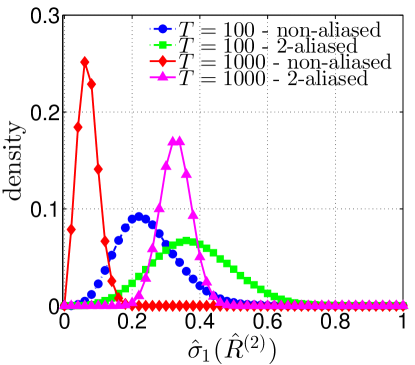
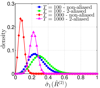
To illustrate the ability of our algorithm to detect aliasing, we generated $T$ outputs from the original aliased HMM and from its non-aliased version $\bar{H}$. Fig.3 (left) shows the empirical densities (averaged over $1000$ independent runs) of the largest singular value of $\hat{R}^{(2)}$, for both $H$ and $\bar{H}$. In Fig.3 (right) we show similar results for a 2A-HMM with $\sigma=0.22$. When $\sigma=0.33$, already $T=1000$ outputs suffice for essentially perfect detection of aliasing. For the smaller $\sigma=0.22$, more samples are required.

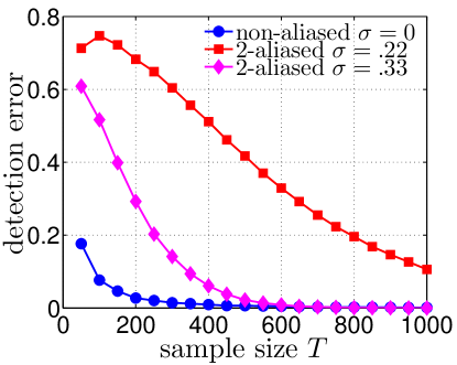
Fig.4 (left) shows the false alarm and misdetection probability vs.​ sample size $T$ of the aliasing detection test (36) with threshold $h_{T}=2T^{-\frac{1}{3}}$. The consistency of our method is evident.

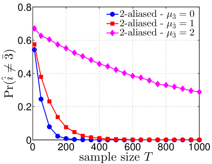
Fig.4 (right) shows the probability of misidentifying the aliased component $\theta_{\bar{3}}$. We considered the same 2A-HMM $H$ but with different means for the Gaussian output distribution of the aliased states, $\mu_{{\bar{3}}}=\{0,1,2\}$. As expected, when $f_{\theta_{\bar{3}}}$ is closer to the output distribution of the non-aliased state $f_{\theta_{1}}$ (with mean $\mu_{1}=3$), identifying the aliased component is more difficult.

Figure 2: The aliased HMM (left) and its corresponding non-aliased version with states $3$ and $4$ merged (right).

Figure 3: Empirical density of the largest singular value of $\hat{R}^{(2)}$ with $\sigma=0.33$ (left) and $\sigma=0.22$ (right).

Figure 4: Misdetection probability of aliasing/non-aliasing (left) and probability of misidentifying the correct aliased component (right).

Figure 5: Average error $\text{{\bf E}}||\hat{A}-A||^{2}_{\textrm{{\tiny{F}}}}$ and runtime comparison of different algorithms vs. sample size $T$.

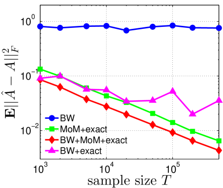
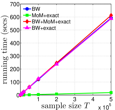
Finally, to estimate $A$ we considered the following methods: The Baum-Welch algorithm with random initial guess of the HMM parameters (BW); our method of moments with exactly known $\bar{\boldsymbol{\theta}}$ (MoM+Exact); BW initialized with the output of our method (BW+MoM+Exact); and BW with exactly known output distributions but random initial guess of the transition matrix (BW+Exact).

Fig.5 (left) shows on a logarithmic scale the mean square error $\text{{\bf E}}||\hat{A}-A||_{F}^{2}$ vs. sample size $T$, averaged over 100 independent realizations. Fig.5 (right) shows the running time as a function of $T$. In these two figures, the number of iterations of the BW was set to 20.

These results show that with a random initial guess of the HMM parameters, BW requires far more than 20 iterations to converge. Even with exact knowledge of the output distributions but a random initial guess for the transition matrix, BW still fails to converge after 20 iterations. In contrast, our method yields a relatively accurate estimator in only a fraction of run-time. For an improved accuracy, this estimator can further be used as an initial guess for $A$ in the BW algorithm.

Appendix A Proofs for Section 3 (Decomposing $A$)

Proof of Lemma 1.

Writing each term in the decomposition (14) explicitly and summing these together we find a match between all entries to those of $A$.

As a representative example let us consider the last entry $A_{n,n}=P(n\,|\,n)$. The first term gives

$$(C_{\beta}\bar{A}B)_{[n,n]}=(1-\beta)P(\bar{n}\,|\,n).$$

The second term gives

$$(C_{\beta}{{\boldsymbol{\delta}}^{\operatorname{out}}}\boldsymbol{c}_{\beta}^{{\textrm{\tiny{T}}}})_{[n,n]} = -\beta(1\!-\!\beta){\delta}^{\operatorname{out}}_{n\!-\!1}$$

$$= -\beta(1\!-\!\beta)(P(\bar{n}\,|\,n\!-\!1)\!-\!P(\bar{n}\,|\,n)).$$

The third term,

$$(\boldsymbol{b}({{\boldsymbol{\delta}}^{\operatorname{in}}})^{{\textrm{\tiny{T}}}}B)_{[n,n]} = -{\delta}^{\operatorname{in}}_{n\!-\!1}$$

$$= -\beta(\alpha_{n\!-\!1}\!-\!\beta)P(\bar{n}\,|\,n\!-\!1)$$

$$-\,(1\!-\!\beta)(\alpha_{n}\!-\!\beta)P(\bar{n}\,|\,n).$$

And lastly, the fourth term gives

$$(\kappa\boldsymbol{b}\boldsymbol{c}_{\beta}^{{\textrm{\tiny{T}}}})_{[n,n]} = \beta(\alpha_{n\!-\!1}-\beta)P(\bar{n}\,|\,n\!-\!1)$$

$$-\,\beta(\alpha_{n}-\beta)P(\bar{n}\,|\,n).$$

Putting $P(\bar{n}\,|\,n)=P(n\!-\!1\,|\,n)+P(n\,|\,n)$ and $P(\bar{n}\,|\,n\!-\!1)=P(n\!-\!1\,|\,n\!-\!1)+P(n\,|\,n\!-\!1)$, and summing all these four terms we obtain $P(n\,|\,n)$ as needed. The other entries of $A$ are obtained similarly. ∎

Appendix B Proofs for Section 4.1 (Minimality)

Let $H=(A,\boldsymbol{\theta},\boldsymbol{\pi}^{0})$ be a 2A-HMM. For any $k\geq 1$ the distribution $P_{H,k}\in\mathcal{P}_{H}$ can be cast in an explicit matrix form. Let $o\in\mathcal{Y}$. The observable operator $T_{\boldsymbol{\theta}}(o)\in\mathbb{R}^{n\times n}$ is defined by

$$T_{\boldsymbol{\theta}}(o)=\operatorname{diag}\left(f_{\theta_{1}}(o),f_{\theta_{2}}(o),\dots,f_{\theta_{n}}(o)\right).$$

Let $y=(y_{0},y_{1},\dots,y_{k-1})\in\mathcal{Y}^{k}$ be a sequence of $k\geq 1$ initial consecutive observations. Then the distribution $P_{H,k}(y)$ is given by Jaeger [2000],

$$P_{H,k}(y)=\boldsymbol{1}_{n}^{\textrm{\tiny{T}}}T_{\boldsymbol{\theta}}(y_{k-1})A\,\dots A\,T_{\boldsymbol{\theta}}(y_{1})A\,T_{\boldsymbol{\theta}}(y_{0})\boldsymbol{\pi}^{0}.$$ (43)

Proof of Theorem 1..

Let us first show that ${{\boldsymbol{\delta}}^{\operatorname{out}}}\neq 0$ is necessary for minimality, namely if ${{\boldsymbol{\delta}}^{\operatorname{out}}}=0$ then $H$ is not minimal, regardless of the initial distribution $\boldsymbol{\pi}^{0}$. The non-minimality will be shown by explicitly constructing a $n\!-\!1$ state HMM equivalent to $H$. Let us denote the lifting of the merged transition matrix by

$$\tilde{A}=C_{\beta}\bar{A}B\in\mathbb{R}^{n\times n}.$$

Assume that ${{\boldsymbol{\delta}}^{\operatorname{out}}}=0$. We will shortly see that for any $\boldsymbol{\pi}^{0}$ and for any $k\geq 2$ consecutive observations $y=(y_{0},y_{1},\dots,y_{k-1})\in\mathcal{Y}^{k}$ we have that

$$T_{\boldsymbol{\theta}}(y_{k-1})A\dots T_{\boldsymbol{\theta}}(y_{1})AT_{\boldsymbol{\theta}}(y_{0})\boldsymbol{\pi}^{0}$$

$$- T_{\boldsymbol{\theta}}(y_{k-1})\tilde{A}\dots T_{\boldsymbol{\theta}}(y_{1})\tilde{A}T_{\boldsymbol{\theta}}(y_{0})\boldsymbol{\pi}^{0}\,\propto\,{\boldsymbol{b}}.$$

Combining (B) with (43), and the fact that $\boldsymbol{1}_{n}^{\textrm{\tiny{T}}}\boldsymbol{b}=0$, we have that $\mathcal{P}_{(A,\boldsymbol{\theta},\boldsymbol{\pi}^{0})}=\mathcal{P}_{(\tilde{A},\boldsymbol{\theta},\boldsymbol{\pi}^{0})}$. Since $\tilde{A}$ has identical $(n\!-\!1)$-th and $n$-th columns, and $f_{\theta_{n\!-\!1}}=f_{\theta_{n}}$ we have that $\mathcal{P}_{(\tilde{A},\boldsymbol{\theta},\boldsymbol{\pi}^{0})}=\mathcal{P}_{(\bar{A},\bar{\boldsymbol{\theta}},\bar{\boldsymbol{\pi}}^{0})}$. Thus $H^{\prime}=(\bar{A},\bar{\boldsymbol{\theta}},\bar{\boldsymbol{\pi}}^{0})$ is an equivalent $(n\!-\!1)$-state HMM and $H$ is not minimal, proving the claim. We prove (B) by induction on the sequence length $k\geq 2$. First note that since ${{\boldsymbol{\delta}}^{\operatorname{out}}}=0$, by Lemma 1 we have that

$$A=\tilde{A}+\boldsymbol{b}(({{\boldsymbol{\delta}}^{\operatorname{in}}})^{\textrm{\tiny{T}}}B+\kappa\boldsymbol{c}_{\beta}^{\textrm{\tiny{T}}}).$$

Since for any $y\in\mathcal{Y}$, $T_{\boldsymbol{\theta}}(y)\boldsymbol{b}=f_{\theta_{\bar{n}}}(y)\boldsymbol{b}$, we have that

$$T_{\boldsymbol{\theta}}(y)A-T_{\boldsymbol{\theta}}(y)\tilde{A}=f_{\theta_{\bar{n}}}(y)\boldsymbol{b}(({{\boldsymbol{\delta}}^{\operatorname{in}}})^{\textrm{\tiny{T}}}B+\kappa\boldsymbol{c}_{\beta}^{\textrm{\tiny{T}}})\propto\,{\boldsymbol{b}}.$$

This proves the case $k=2$. Next, assume (B) holds for all sequences of length at least 2 and smaller than $k$, namely, for some $a\in\mathbb{R}$

$$T_{\boldsymbol{\theta}}(y_{k-2})A\dots T_{\boldsymbol{\theta}}(y_{1})AT_{\boldsymbol{\theta}}(y_{0})\boldsymbol{\pi}^{0}$$

$$= a{\boldsymbol{b}}+T_{\boldsymbol{\theta}}(y_{k-2})\tilde{A}\dots T_{\boldsymbol{\theta}}(y_{1})\tilde{A}T_{\boldsymbol{\theta}}(y_{0})\boldsymbol{\pi}^{0}.$$

Using the fact that $B\boldsymbol{b}=0$ we have $T_{\boldsymbol{\theta}}(y_{k\!-\!1})\tilde{A}\boldsymbol{b}=0$. Inserting the expansion of $A$ in the l.h.s of (B) we get

$$f_{\theta_{\bar{n}}}(y_{k\!-\!1})\boldsymbol{b}\left(({{\boldsymbol{\delta}}^{\operatorname{in}}})^{\textrm{\tiny{T}}}B+\kappa\boldsymbol{c}_{\beta}^{\textrm{\tiny{T}}}\right)$$

$$\times \left(a\boldsymbol{b}+\tilde{A}T_{\boldsymbol{\theta}}(y_{k-2})\dots T_{\boldsymbol{\theta}}(y_{1})\tilde{A}T_{\boldsymbol{\theta}}(y_{0})\boldsymbol{\pi}^{0}\right).$$

Since this last expression is proportional to $\boldsymbol{b}$ we are done.

(ii) The case $\pi^{0}_{\bar{n}}=0$ or $\beta^{0}=\beta$.

As we just saw, having ${{\boldsymbol{\delta}}^{\operatorname{out}}}=0$ implies that the HMM is not minimal. We now show that if ${{\boldsymbol{\delta}}^{\operatorname{in}}}=0$ then $H$ is not minimal either. By contraposition this will prove the first direction of (ii).

So assume that ${{\boldsymbol{\delta}}^{\operatorname{in}}}=0$. Lemma 1 implies

$$A=\tilde{A}+({C_{\beta}}({{\boldsymbol{\delta}}^{\operatorname{out}}})+\kappa\boldsymbol{b})\boldsymbol{c}_{\beta}^{\textrm{\tiny{T}}}.$$ (45)

Now note that for all $y\in\mathcal{Y}$,  $\boldsymbol{c}_{\beta}^{\textrm{\tiny{T}}}T_{\boldsymbol{\theta}}(y)=f_{\theta_{n\!-\!1}}(y)\boldsymbol{c}_{\beta}^{\textrm{\tiny{T}}}$ and since either $\pi^{0}_{\bar{n}}=0$ or $\beta^{0}=\beta$ we have that $\boldsymbol{c}_{\beta}^{\textrm{\tiny{T}}}\boldsymbol{\pi}^{0}=0$. Thus $\boldsymbol{c}_{\beta}T_{\boldsymbol{\theta}}(y)\boldsymbol{\pi}^{0}=0$ and we find that

$$T_{\boldsymbol{\theta}}(y_{k-1})A\dots AT_{\boldsymbol{\theta}}(y_{1})AT_{\boldsymbol{\theta}}(y_{0})\boldsymbol{\pi}^{0}$$ (46)

$$\qquad=T_{\boldsymbol{\theta}}(y_{k-1})A\dots AT_{\boldsymbol{\theta}}(y_{1})\tilde{A}T_{\boldsymbol{\theta}}(y_{0})\boldsymbol{\pi}^{0}.$$ (47)

Now since $\boldsymbol{c}_{\beta}^{\textrm{\tiny{T}}}C_{\beta}=0$ we have that for any $y\in\mathcal{Y}$, $\boldsymbol{c}_{\beta}^{\textrm{\tiny{T}}}T_{\boldsymbol{\theta}}(y)\tilde{A}=0$ and thus expanding $A$ by (45) we find that for any $y\in\mathcal{Y}$,

$$AT_{\boldsymbol{\theta}}(y)\tilde{A}=\Big{(}\tilde{A}+({C_{\beta}}({{\boldsymbol{\delta}}^{\operatorname{out}}})+\kappa\boldsymbol{b})\boldsymbol{c}_{\beta}^{\textrm{\tiny{T}}}\Big{)}T_{\boldsymbol{\theta}}(y)\tilde{A}=\tilde{A}T_{\boldsymbol{\theta}}(y)\tilde{A}.$$

Thus each $A$ in the right hand side of (46) can be replaced by $\tilde{A}$ and we conclude that $\mathcal{P}_{(A,\boldsymbol{\theta},\boldsymbol{\pi}^{0})}=\mathcal{P}_{(\tilde{A},\boldsymbol{\theta}_{n},\boldsymbol{\pi}^{0})}$. Similarly to the case ${{\boldsymbol{\delta}}^{\operatorname{out}}}=0$ we have that $H^{\prime}=(\bar{A},\bar{\boldsymbol{\theta}},\bar{\boldsymbol{\pi}}^{0})$ is an equivalent $(n\!-\!1)$-state HMM and thus $H$ is not minimal.

In order to prove the other direction we will show that if $H$ is not minimal then either ${{\boldsymbol{\delta}}^{\operatorname{out}}}=0$ or ${{\boldsymbol{\delta}}^{\operatorname{in}}}=0$. This is equivalent to the condition ${{\boldsymbol{\delta}}^{\operatorname{out}}}{{\boldsymbol{\delta}}^{\operatorname{in}}}^{{\textrm{\tiny{T}}}}=0$.

Assuming $H$ is not minimal, there exists an HMM ${H^{\prime}}$ with ${n^{\prime}}<n$ states such that $\mathcal{P}_{H^{\prime}}=\mathcal{P}_{H}$. Assumptions (A1-A3) readily imply that $H^{\prime}$ must have $n^{\prime}=n\!-\!1$ states and that the unique $n\!-\!1$ output components are identical for $H$ and $H^{\prime}$. Since $\mathcal{P}_{H^{\prime}}$ is invariant to permutations, we may assume that $\bar{\boldsymbol{\theta}}^{\prime}=\bar{\boldsymbol{\theta}}$ and consequently the kernel matrices in (1) for both $H$ and $H^{\prime}$ are equal ${\bar{K}}={\bar{K}}^{\prime}$.

Let $A^{\prime}\in\mathbb{R}^{(n\!-\!1)\times(n\!-\!1)}$ be the transition matrix of $H^{\prime}$ and define $H^{\prime\prime}=(A^{\prime\prime},\boldsymbol{\theta}^{\prime\prime},\pi^{\prime\prime})$ as the equivalent $n$-state HMM to $H^{\prime}$ by setting $\beta^{\prime\prime}=\beta$, $A^{\prime\prime}=C_{\beta}A^{\prime}B$, $\boldsymbol{\theta}^{\prime\prime}=\bar{\boldsymbol{\theta}}^{\prime}B$ and $\boldsymbol{\pi}^{\prime\prime}=C_{\beta}\bar{\boldsymbol{\pi}}^{\prime}$. Note that for $H^{\prime\prime}$, by construction we have ${{\boldsymbol{\delta}}^{\operatorname{out}}}^{\prime\prime}({{\boldsymbol{\delta}}^{\operatorname{in}}}^{\prime\prime}){{}^{\textrm{\tiny{T}}}}=0$.

Now, by the equivalence of the two models $H$ and $H^{\prime\prime}$, we have that the second order moments ${{\mathcal{M}}}^{(2)}$ given in (19) are the same for both. By the fact that ${\bar{K}}^{\prime\prime}={\bar{K}}$, $\bar{\boldsymbol{\pi}}^{\prime\prime}=\bar{\boldsymbol{\pi}}$ and by (29) in Lemma 3 we must have that ${{\boldsymbol{\delta}}^{\operatorname{out}}}{({{\boldsymbol{\delta}}^{\operatorname{in}}})}^{\textrm{\tiny{T}}}={{\boldsymbol{\delta}}^{\operatorname{out}}}^{\prime\prime}({{\boldsymbol{\delta}}^{\operatorname{in}}}^{\prime\prime}){{}^{\textrm{\tiny{T}}}}$. Thus ${{\boldsymbol{\delta}}^{\operatorname{out}}}{({{\boldsymbol{\delta}}^{\operatorname{in}}})}^{\textrm{\tiny{T}}}=0$ and the claim is proved.

(i) The case $\pi^{0}_{\bar{n}}\neq 0$ and $\beta^{0}\neq\beta$.

We saw above that if $H$ is minimal then ${{\boldsymbol{\delta}}^{\operatorname{out}}}\neq 0$. Thus, in order to prove the claim we are left to show that if $H$ is not minimal then ${{\boldsymbol{\delta}}^{\operatorname{out}}}=0$.

So assume $H$ is not minimal and let $H^{\prime\prime}$ be constructed as above. By way of contradiction assume ${{\boldsymbol{\delta}}^{\operatorname{out}}}\neq 0$. As we just saw, since $H$ is not minimal then ${{\boldsymbol{\delta}}^{\operatorname{out}}}({{\boldsymbol{\delta}}^{\operatorname{in}}})^{{\textrm{\tiny{T}}}}$ = 0. Thus by the assumption ${{\boldsymbol{\delta}}^{\operatorname{out}}}\neq 0$ we must have ${{\boldsymbol{\delta}}^{\operatorname{in}}}=0$. This implies that $A$ is in the form (45). Since $\mathcal{P}_{H}=\mathcal{P}_{H^{\prime\prime}}$ we have $P_{H,2}=P_{H^{\prime\prime},2}$ where:

$$P_{H,2} = \boldsymbol{1}_{n}^{\textrm{\tiny{T}}}T_{\boldsymbol{\theta}}(y_{2})AT_{\boldsymbol{\theta}}(y_{1})\boldsymbol{\pi}^{0}$$

$$= \boldsymbol{1}_{n}^{\textrm{\tiny{T}}}T_{\boldsymbol{\theta}}(y_{2})\Big{(}\tilde{A}+({C_{\beta}}{{\boldsymbol{\delta}}^{\operatorname{out}}}+\kappa\boldsymbol{b})\boldsymbol{c}_{\beta}^{\textrm{\tiny{T}}}\Big{)}T_{\boldsymbol{\theta}}(y_{1})\boldsymbol{\pi}^{0}$$

$$P_{H^{\prime\prime},2} = \boldsymbol{1}_{n}^{\textrm{\tiny{T}}}T_{\boldsymbol{\theta}}(y_{2})A^{\prime\prime}T_{\boldsymbol{\theta}}(y_{1})\boldsymbol{\pi}^{0}.$$

In addition, by the fact that ${\bar{K}}^{\prime\prime}={\bar{K}}$, $\bar{\boldsymbol{\pi}}^{\prime\prime}=\bar{\boldsymbol{\pi}}$ we must have that ${M}^{(1)}={{M}^{\prime\prime}}^{(1)}$, where ${M}^{(1)}$ is defined in (23) and ${{M}^{\prime\prime}}^{(1)}$ is defined similarly with the parameters of $H^{\prime\prime}$ instead of $H$. By (28) in Lemma 3 we thus have

$${{M}^{\prime\prime}}^{(1)}=A^{\prime}=\bar{A}={{M}}^{(1)}.$$

Hence $A^{\prime\prime}=\tilde{A}$ and $P_{H,2}=P_{H^{\prime\prime},2}$ is equivalent to

$$\boldsymbol{1}_{n}^{\textrm{\tiny{T}}}T_{\boldsymbol{\theta}}(y_{2})\Big{(}{C_{\beta}}{{\boldsymbol{\delta}}^{\operatorname{out}}}+\kappa\boldsymbol{b}\Big{)}\boldsymbol{c}_{\beta}^{\textrm{\tiny{T}}}T_{\boldsymbol{\theta}}(y_{1})\boldsymbol{\pi}^{0}=0.$$ (48)

Now, note that $\forall y_{1},y_{2}\in\mathcal{Y}$ we have

$$\boldsymbol{1}_{n}^{\textrm{\tiny{T}}}T_{\boldsymbol{\theta}}(y_{2})\boldsymbol{b} = 0$$

$$\boldsymbol{c}_{\beta}^{\textrm{\tiny{T}}}T_{\boldsymbol{\theta}}(y_{1})\boldsymbol{\pi}^{0} = (\beta^{0}-\beta)\pi^{0}_{\bar{n}}f_{\theta_{\bar{n}}}(y_{1})$$

$$\boldsymbol{1}_{n}^{\textrm{\tiny{T}}}T_{\boldsymbol{\theta}}(y_{2}){C_{\beta}} = (f_{\theta_{1}}(y_{2}),\dots,f_{\theta_{n\!-\!1}}(y_{2})).$$

Thus, (48) is given by

$$(\beta^{0}-\beta)\pi^{0}_{\bar{n}}f_{\theta_{n\!-\!1}}(y_{1})\Big{(}f_{\theta_{1}}(y_{2}),\dots,f_{\theta_{n\!-\!1}}(y_{2})\Big{)}\cdot{{\boldsymbol{\delta}}^{\operatorname{out}}}=0.$$

Since by assumption $(\beta^{0}-\beta)\pi^{0}_{\bar{n}}\neq 0$ we have $\forall y_{1},y_{2}\in\mathcal{Y}$

$$f_{\theta_{n\!-\!1}}(y_{1})\Big{(}f_{\theta_{1}}(y_{2}),\dots,f_{\theta_{n\!-\!1}}(y_{2})\Big{)}\cdot{{\boldsymbol{\delta}}^{\operatorname{out}}}=0.$$

For each $i\in[n\!-\!1]$, multiplying by $f_{\theta_{i}}(y_{2})$ and integrating over $y_{1},y_{2}\in\mathcal{Y}$ we get

$${\bar{K}}{{\boldsymbol{\delta}}^{\operatorname{out}}}=0.$$

Since ${\bar{K}}$ is full rank we must have ${{\boldsymbol{\delta}}^{\operatorname{out}}}=0$ in contradiction to the assumption ${{\boldsymbol{\delta}}^{\operatorname{out}}}\neq 0$. This concludes the proof of the Theorem. ∎

Appendix C Proofs for Section 4.2 (Identifiability)

Figure 6: The feasible region $\Gamma_{H}$ (shaded) in the $(\tau_{n\!-\!1},\tau_{n})$ plane. Any $(\tau_{n\!-\!1},\tau_{n})\in\Gamma_{H}$ induces an HMM equivalent to $H$ via Lemma 2. The pair $(\tau_{n\!-\!1},\tau_{n})=(1,0)$, corresponding to the original transition matrix $A$, is indicated by a yellow point. Left: $\alpha_{n\!-\!1}\geq\alpha_{n}$ and Right: $\alpha_{n\!-\!1}<\alpha_{n}$.

C.1 Proof of Theorem 2

Figure 7: Top: Plotting the columns of $BA$ on the simplex for a 2A-HMM with aliased states $\{3,4\}$. Here, $\bar{\boldsymbol{a}}_{\bar{3}}=\beta\bar{\boldsymbol{a}}_{3}+(1-\beta)\bar{\boldsymbol{a}}_{4}$. Bottom: Any vectors $\bar{\boldsymbol{a}}_{H,n\!-\!1},\bar{\boldsymbol{a}}_{H,n}$ within the depicted bars results in a matrix $A_{H}$ with all entries non-negative, except in possibly the $2\times 2$ aliased block.

Before characterizing $\Gamma_{H}$ let us first give some intuition on the role of $(\tau_{n\!-\!1},\tau_{n})$. Consider the ${n\!-\!1}$ dimensional columns $\{\bar{\boldsymbol{a}}_{i}\,|\,i\in[n]\}$ of the matrix $BA$. These can be plotted on the $n\!-\!1$ dimensional simplex, as shown in Fig.7 (top), for $n=4$ and aliased states $\{3,4\}$. Recall that

$$A_{H}(\tau_{n\!-\!1},\tau_{n})=S(\tau_{n\!-\!1},\tau_{n})^{-1}AS(\tau_{n\!-\!1},\tau_{n})$$

and let $\{\bar{\boldsymbol{a}}_{H,i}\,|\,i\in[n]\}$ be the columns of the matrix $BA_{H}\in\mathbb{R}^{{n\!-\!1}\times n}$.

Since $BS(\tau_{n\!-\!1},\tau_{n})^{-1}=B$ we have $BA_{H}=BAS(\tau_{n\!-\!1},\tau_{n}).$ So the non-aliased columns of $BA_{H}$ are unaltered from these of $BA$, i.e. for all $i\in[n\!-\!2]$, $\bar{\boldsymbol{a}}_{i}=\bar{\boldsymbol{a}}_{H,i}$. The new aliased columns of $BA_{H}$ are

$${\bar{\boldsymbol{a}}_{H,n\!-\!1}} = {{\bar{\boldsymbol{a}}}_{n}}+\tau_{n\!-\!1}{{\boldsymbol{\delta}}^{\operatorname{out}}}$$

$${\bar{\boldsymbol{a}}_{H,n}} = {{\bar{\boldsymbol{a}}}_{n}}+\tau_{n}{{\boldsymbol{\delta}}^{\operatorname{out}}}.$$

Thus $\tau_{n\!-\!1}$ ($\tau_{n}$) determines the position of the vector $\bar{\boldsymbol{a}}_{H,n\!-\!1}$ ($\bar{\boldsymbol{a}}_{H,n}$) along the ray passing through $\bar{\boldsymbol{a}}_{n\!-\!1}$ and $\bar{\boldsymbol{a}}_{n}$ (dashed line in Fig.7).

Hence a necessary condition for $A_{H}$ to be a valid transition matrix is that ${\bar{\boldsymbol{a}}_{H,n\!-\!1}\geq 0}$ and ${\bar{\boldsymbol{a}}_{H,n}\geq 0}$, and one cannot take $\tau_{n\!-\!1}$ and $\tau_{n}$ arbitrarily. In particular, there are $\tau^{\max}_{n\!-\!1}$ and $\tau^{\max}_{n}$ such that $\bar{\boldsymbol{a}}_{H,n\!-\!1}$ and $\bar{\boldsymbol{a}}_{H,n}$ are as “far” apart as possible by putting them on the opposite sides of the ray connecting them, such that both sit on the simplex boundary. This is achieved by taking

$${\bar{\boldsymbol{a}}^{\max}_{H,n\!-\!1}} = {{\bar{\boldsymbol{a}}}_{n}}+\tau^{\max}_{n\!-\!1}{{\boldsymbol{\delta}}^{\operatorname{out}}}$$

$${\bar{\boldsymbol{a}}^{\max}_{H,n}} = {{\bar{\boldsymbol{a}}}_{n}}+\tau^{\max}_{n}{{\boldsymbol{\delta}}^{\operatorname{out}}},$$

where

$$\tau^{\max}_{n\!-\!1}= \min_{j\in\mathcal{X}\setminus\{{n\!-\!1},n\}}\frac{\frac{1}{2}(1+\operatorname{sign}({\delta}^{\operatorname{out}}_{j}))-({\bar{\boldsymbol{a}}_{n}})_{j}}{{\delta}^{\operatorname{out}}_{j}} \geq 0$$

$$\tau^{\max}_{n}= \max_{j\in\mathcal{X}\setminus\{{n\!-\!1},n\}}\frac{\frac{1}{2}(1-\operatorname{sign}({\delta}^{\operatorname{out}}_{j}))-({\bar{\boldsymbol{a}}_{n}})_{j}}{{\delta}^{\operatorname{out}}_{j}} \leq 0.$$

(see Fig.7, bottom). Since we assumed as a convention that $\tau_{n\!-\!1}>\tau_{n}$ we have that any $\tau_{n\!-\!1}\leq\tau_{n\!-\!1}^{\max}$ and $\tau_{n}\geq\tau_{n}^{\max}$ results in a non negative matrix $BA_{H}$. Note that $BA_{H}\geq 0$ implies ${A_{H}}_{[1:n\!-\!2,1:n]}\geq 0$.

Next, consider the new relative probabilities $\alpha_{H,i}$ as defined by (10) with $A_{H}$ replacing $A$. One can verify that these satisfy

$$\alpha_{H,i}=\frac{\alpha_{i}-\tau_{n}}{\tau_{{n\!-\!1}}-\tau_{n}},\quad i\in\operatorname{supp}_{{\textrm{\tiny{in}}}}\backslash\{{n\!-\!1},n\}.$$

Obviously, a necessary condition for $A_{H}$ to be a valid transition matrix is that

$$0\leq\alpha_{H,i}=\frac{\alpha_{i}-\tau_{n}}{\tau_{{n\!-\!1}}-\tau_{n}}\leq 1,\quad i\in\operatorname{supp}_{{\textrm{\tiny{in}}}}\backslash\{{n\!-\!1},n\}.$$ (49)

Define the minimal and maximal relative probabilities of the non-aliased states by

$$\alpha^{\min} = \min\,\{\alpha_{i}\,|\,i\in\operatorname{supp}_{{\textrm{\tiny{in}}}}\backslash\{{n\!-\!1},n\}\}$$

$$\alpha^{\max} = \max\,\{\alpha_{i}\,|\,i\in\operatorname{supp}_{{\textrm{\tiny{in}}}}\backslash\{{n\!-\!1},n\}\}.$$

Let $\alpha^{\min}_{H}$ and $\alpha^{\max}_{H}$ be defined similarly. Taking

$$\tau^{\min}_{n\!-\!1} = \alpha^{\max}$$

$$\tau^{\min}_{n} = \alpha^{\min},$$

we have $\alpha^{\min}_{H}=0$ and $\alpha^{\max}_{H}=1$. Hence, for any $\tau_{n\!-\!1}\geq\tau^{\min}_{n\!-\!1}$ and $\tau_{n}\leq\tau^{\min}_{n}$ the constraint (49) holds and consequently ${A_{H}}_{[1:n,1:n\!-\!2]}$ is non-negative. The corresponding columns $\bar{\boldsymbol{a}}_{H,n\!-\!1}^{\min}={{\bar{\boldsymbol{a}}}_{n}}+\tau^{\min}_{n\!-\!1}{{\boldsymbol{\delta}}^{\operatorname{out}}}$ and $\bar{\boldsymbol{a}}_{H,n}^{\min}={{\bar{\boldsymbol{a}}}_{n}}+\tau^{\min}_{n}{{\boldsymbol{\delta}}^{\operatorname{out}}}$ are depicted in Fig.7 (bottom).

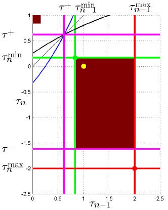
Combining the above constraints we have that the four parameters $\tau^{\min}_{n\!-\!1},\tau^{\min}_{n},\tau^{\max}_{n\!-\!1},\tau^{\max}_{n}$ define the rectangle

$$\Gamma_{1}=[\tau^{\min}_{n\!-\!1},\tau^{\max}_{n\!-\!1}]\times[\tau^{\max}_{n},\tau^{\min}_{n}],$$ (50)

which characterize the equivalent matrices $A_{H}$ having all entries non-negative except of possibly in the $2\times 2$ aliased block (see Fig.6). Thus we must have $\Gamma_{H}\subset\Gamma_{1}$.

We are left to find the conditions under which the $2\times 2$ aliased block is non-negative. Writing $A_{H}$ explicitly we have that these conditions are

$$A_{H,n,{n\!-\!1}} = \tau_{n\!-\!1}(\tau_{n\!-\!1}-\alpha_{n\!-\!1})P(\bar{n}\,|\,{n\!-\!1})$$

$$+\,(1-\tau_{n\!-\!1})(\tau_{n\!-\!1}-\alpha_{n})P(\bar{n}\,|\,n)\geq 0$$

$$A_{H,{n\!-\!1},n} = \tau_{n}(\alpha_{n\!-\!1}-\tau_{n})P(\bar{n}\,|\,{n\!-\!1})$$

$$+\,(1-\tau_{n})(\alpha_{n}-\tau_{n})P(\bar{n}\,|\,n)\geq 0$$

$$A_{H,{n\!-\!1},{n\!-\!1}} = \tau_{n\!-\!1}(\alpha_{n\!-\!1}\!-\!\tau_{n})P(\bar{n}\,|\,{n\!-\!1})$$

$$+\,(1\!-\!\tau_{n\!-\!1})(\alpha_{n}-\tau_{n})P(\bar{n}\,|\,n)\geq 0$$

$$A_{H,n,n} = \tau_{n}(\tau_{n\!-\!1}-\alpha_{n\!-\!1})P(\bar{n}\,|\,{n\!-\!1})$$

$$+\,(1-\tau_{n})(\tau_{n\!-\!1}-\alpha_{n})P(\bar{n}\,|\,n)\geq 0.$$

As the case $P(\bar{n}\,|\,{n\!-\!1})=P(\bar{n}\,|\,n)=0$ is trivial, we assume that at least one of $P(\bar{n}\,|\,{n\!-\!1}),P(\bar{n}\,|\,n)$ is nonzero (and since by convention $P(\bar{n}\,|\,{n\!-\!1})\geq P(\bar{n}\,|\,n)$, this is equivalent to $P(\bar{n}\,|\,{n\!-\!1})>0$).

Recall that by definition ${\delta}^{\operatorname{out}}_{n\!-\!1}=P(\bar{n}\,|\,{n\!-\!1})-P(\bar{n}\,|\,n)$ (see (11)). We now consider the cases ${\delta}^{\operatorname{out}}_{n\!-\!1}=0$ and ${\delta}^{\operatorname{out}}_{n\!-\!1}>0$ separately.

The case ${\delta}^{\operatorname{out}}_{n\!-\!1}=0$.

Consider first the off-diagonal constraint (C.1) for $A_{H,{n\!-\!1},n}\geq 0$, taking the form

$$\tau_{n}(1-(\alpha_{n\!-\!1}-\alpha_{n})))\leq\alpha_{n}.$$

Denote

$$\tau^{0}={\alpha_{n}}/{(1-(\alpha_{n\!-\!1}-\alpha_{n}))}.$$

Since $\alpha_{n\!-\!1}-\alpha_{n}\leq 1$ we need $\tau_{n}\leq\tau^{0}.$ Similarly, (C.1) is satisfied if and only if $\tau_{n\!-\!1}\geq\tau^{0}.$ Thus in order for the off-diagonal entries $A_{H,n,{n\!-\!1}},A_{H,{n\!-\!1},n}$ to be non-negative we need $(\tau_{n\!-\!1},\tau_{n})\in\Gamma_{2}^{0}$ where

$$\Gamma_{2}^{0}=[\tau^{0},\infty]\times[-\infty,\tau^{0}].$$ (55)

Next, the on-diagonal constraint (C.1) for $A_{H,{n\!-\!1},{n\!-\!1}}\geq 0$ is equivalent to

$$\tau_{n}\leq\alpha_{n}+\tau_{n\!-\!1}(\alpha_{n\!-\!1}-\alpha_{n}).$$ (56)

Similarly, the on-diagonal constrain (C.1) for $A_{H,n,n}\geq 0$ is

$$\tau_{n}(\alpha_{n\!-\!1}-\alpha_{n})\leq\tau_{n\!-\!1}-\alpha_{n}.$$ (57)

Define the two linear functions $g^{0},f^{0}:\mathbb{R}\to\mathbb{R}$ by

$$g^{0}(\tau_{n\!-\!1}) = \alpha_{n}+\tau_{n\!-\!1}(\alpha_{n\!-\!1}-\alpha_{n})$$

$$f^{0}(\tau_{n\!-\!1}) = \frac{\tau_{n\!-\!1}-\alpha_{n}}{\alpha_{n\!-\!1}-\alpha_{n}}.$$

Note that $\tau^{0}$ is a fixed point of both $g^{0}$ and $f^{0}$,

$$\tau^{0}=g^{0}(\tau^{0})=f^{0}(\tau^{0}).$$

Note also that for $\alpha_{n\!-\!1}\geq\alpha_{n}$ the functions $g^{0}$ and $f^{0}$ are increasing, while for $\alpha_{n\!-\!1}<\alpha_{n}$ they are decreasing. Thus, if $\alpha_{n\!-\!1}\geq\alpha_{n}$ the constrains (56,57) are automatically satisfied for $(\tau_{n\!-\!1},\tau_{n})\in\Gamma_{2}^{0}$, so in this case $A_{H,{n\!-\!1},{n\!-\!1}},A_{H,n,n}$ are also guaranteed to be non-negative.

If $\alpha_{n\!-\!1}<\alpha_{n}$ then with $\tau_{n\!-\!1}\geq\tau_{n}$ (as we assume here) we have $f^{0}(\tau_{n\!-\!1})\leq g^{0}(\tau_{n\!-\!1})\leq\tau_{0}$ and the constraints (56,57) take the form $f^{0}(\tau_{n\!-\!1})\leq\tau_{n}\leq g^{0}(\tau_{n\!-\!1}).$ Thus, in order for the on-diagonal entries $A_{H,{n\!-\!1},{n\!-\!1}}$ and $A_{H,n,n}$ to be non-negative we must have $(\tau_{n\!-\!1},\tau_{n})\in\Gamma_{3}^{0}$, where

$$\Gamma_{3}^{0}=\{(\tau_{n\!-\!1},\tau_{n})\in\Gamma_{1}\,|\,f^{0}(\tau_{n\!-\!1})\leq\tau_{n}\leq g^{0}(\tau_{n\!-\!1})\}.$$ (58)

We are left to ensure that for $\alpha_{n\!-\!1}<\alpha_{n}$ the off diagonal entries are also non-negative. Indeed, since $\tau_{n}\leq\tau_{n\!-\!1}$, $\tau^{0}$ is a fixed point and $g(\tau_{n\!-\!1}),f(\tau_{n\!-\!1})$ are decreasing, for any $(\tau_{n\!-\!1},\tau_{n})\in\Gamma_{3}^{0}$ we automatically have that $\tau_{0}\leq\tau_{n\!-\!1}$ and $\tau_{n}\leq\tau_{0}$, so $(\tau_{n\!-\!1},\tau_{n})\in\Gamma_{3}^{0}$ implies $(\tau_{n\!-\!1},\tau_{n})\in\Gamma_{2}^{0}$. Thus all entries of the aliasing block are guaranteed to be non-negative.

To conclude, we have shown that for ${\delta}^{\operatorname{out}}_{n\!-\!1}=0$ the feasible region (17) is given by

$$\Gamma_{H}^{0}=\begin{cases}\Gamma_{1}\cap\Gamma_{2}^{0}&\alpha_{n\!-\!1}\geq\alpha_{n}\\ \Gamma_{1}\cap\Gamma_{3}^{0}&\alpha_{n\!-\!1}<\alpha_{n}.\end{cases}$$

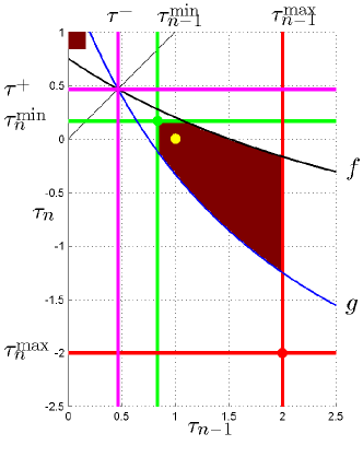
The case ${\delta}^{\operatorname{out}}_{n\!-\!1}>0$.

This case has the same characteristics as for the ${\delta}^{\operatorname{out}}_{n\!-\!1}=0$ case, but it is a bit more complex to analyze. Define $\tau^{\pm}$ (as the analogues of $\tau^{0}$) by

$$\tau^{\pm} = \frac{1}{2{\delta}^{\operatorname{out}}_{n\!-\!1}}\Big{(}\alpha_{n\!-\!1}P(\bar{n}\,|\,{n\!-\!1})$$

$$\hskip 50.0pt-(1+\alpha_{n})P(\bar{n}\,|\,n)\pm{\sqrt{\Delta}}\Big{)},$$

where

$${\Delta} = \Big{(}\alpha_{n\!-\!1}P(\bar{n}\,|\,{n\!-\!1})-(1+\alpha_{n})P(\bar{n}\,|\,n)\Big{)}^{2}$$

$$\hskip 80.0pt+\,4\alpha_{n}P(\bar{n}\,|\,n){\delta}^{\operatorname{out}}_{n\!-\!1}\geq 0.$$

And define the regions

$$\Gamma_{2} \!\!=\!\! [\tau^{+},\infty]\times[\tau^{-},\tau^{+}]$$ (60)

$$\Gamma_{3} \!\!=\!\! \{(\tau_{n\!-\!1},\tau_{n})\in\Gamma_{1}\,|\,\,f(\tau_{n\!-\!1})\leq\tau_{n}\leq g(\tau_{n\!-\!1})\}$$ (61)

where the functions $g,f:\mathbb{R}\to\mathbb{R}$ are given by

$$g(\tau_{n\!-\!1}) = \left(\frac{\alpha_{n\!-\!1}P(\bar{n}\,|\,{n\!-\!1})-\alpha_{n}P(\bar{n}\,|\,n)}{{\delta}^{\operatorname{out}}_{n\!-\!1}}\right)$$

$$-\,\frac{P(\bar{n}\,|\,{n\!-\!1})P(\bar{n}\,|\,n)(\alpha_{n\!-\!1}-\alpha_{n})}{({\delta}^{\operatorname{out}}_{n\!-\!1})^{2}}$$

$$\times\,\left(\tau_{n\!-\!1}-\Big{(}\frac{-P(\bar{n}\,|\,n)}{{\delta}^{\operatorname{out}}_{n\!-\!1}}\Big{)}\right)^{-1}$$

and

$$f(\tau_{n\!-\!1}) = \left(\frac{-P(\bar{n}\,|\,n)}{{\delta}^{\operatorname{out}}_{n\!-\!1}}\right)$$

$$-\,\frac{P(\bar{n}\,|\,{n\!-\!1})P(\bar{n}\,|\,n)(\alpha_{n\!-\!1}-\alpha_{n})}{({\delta}^{\operatorname{out}}_{n\!-\!1})^{2}}$$

$$\times\,\left(\tau_{n\!-\!1}-\Big{(}\frac{\alpha_{n\!-\!1}P(\bar{n}\,|\,{n\!-\!1})-\alpha_{n}P(\bar{n}\,|\,n)}{{\delta}^{\operatorname{out}}_{n\!-\!1}}\Big{)}\right)^{-1}.$$

Lemma 8.

Let $\Gamma_{1}$ be defined in (50) and let $\Gamma_{2}$ and $\Gamma_{3}$ be defined according to whether ${\delta}^{\operatorname{out}}_{n\!-\!1}=0$ (55,58) or not (60,61). Then the feasible region $\Gamma_{H}$ satisfies

$$\Gamma_{H}=\begin{cases}\Gamma_{1}\cap\Gamma_{2}&\alpha_{n\!-\!1}\geq\alpha_{n}\\ \Gamma_{1}\cap\Gamma_{3}&\alpha_{n\!-\!1}<\alpha_{n}.\end{cases}$$

Proof.

As the case ${\delta}^{\operatorname{out}}_{n\!-\!1}=0$ was treated above, we consider the case ${\delta}^{\operatorname{out}}_{n\!-\!1}>0$. Consider first the off diagonal constraint (C.1). Multiplying by $(-1)$, we need to solve the following inequality for $\tau\in\mathbb{R}$,

$$\tau^{2}{\delta}^{\operatorname{out}}_{n\!-\!1}-\tau(\alpha_{n\!-\!1}P(\bar{n}\,|\,{n\!-\!1})$$ (64)

$$\hskip 20.0pt-(1+\alpha_{n})P(\bar{n}\,|\,n))-\alpha_{n}P(\bar{n}\,|\,n)\leq 0.$$

We first solve with equality to find the solutions $\tau^{-},\tau^{+}$ given in (C.1). Thus, since $\Delta\geq 0$ we have that any feasible $\tau_{n}$ must satisfy $\tau^{-}\leq\tau_{n}\leq\tau^{+}.$ Note that the constraint (C.1) for $\tau_{n\!-\!1}$ is the complement of (C.1), and by assumption $\tau_{n\!-\!1}\geq\tau_{n}$, so (C.1) is satisfied iff $\tau^{+}\leq\tau_{n\!-\!1}$. Thus, the region $\Gamma_{2}$ given in (60) indeed characterize the non-negativity of both $A_{{n\!-\!1},n}$ and $A_{n,{n\!-\!1}}$. With some algebra, $\tau^{+}$ and $\tau^{-}$ can be shown to satisfy the following useful relations:

• If $\alpha_{n\!-\!1}\geq\alpha_{n}$ then

  $$-\frac{P(\bar{n}\,|\,{n\!-\!1})}{{\delta}^{\operatorname{out}}_{n\!-\!1}}\leq\tau^{-}\leq 0$$ (65)

  and

  $$0\leq\tau^{+}\leq\frac{\alpha_{n\!-\!1}P(\bar{n}\,|\,{n\!-\!1})-\alpha_{n}P(\bar{n}\,|\,n)}{{\delta}^{\operatorname{out}}_{n\!-\!1}}.$$ (66)

• If $\alpha_{n\!-\!1}<\alpha_{n}$ then

  $$\tau^{-} \leq -\frac{P(\bar{n}\,|\,n)}{{\delta}^{\operatorname{out}}_{n\!-\!1}}$$

  $$\leq \frac{\alpha_{n\!-\!1}P(\bar{n}\,|\,{n\!-\!1})-\alpha_{n}P(\bar{n}\,|\,n)}{{\delta}^{\operatorname{out}}_{n\!-\!1}}\leq\tau^{+}.$$

We proceed to handle the constraints (C.1) and (C.1) corresponding to the region $\Gamma_{3}$. We begin by solving the inequality (C.1):

$$-\tau_{n}(P(\bar{n}\,|\,n)+\tau_{n\!-\!1}{\delta}^{\operatorname{out}}_{n\!-\!1})+\alpha_{n}P(\bar{n}\,|\,n)$$

$$\hskip 20.0pt+\,\tau_{n\!-\!1}(\alpha_{n\!-\!1}P(\bar{n}\,|\,{n\!-\!1})-\alpha_{n}P(\bar{n}\,|\,n))\geq 0.$$

Note that for $(\tau_{n\!-\!1},\tau_{n})\in\Gamma_{1}$ we have $(P(\bar{n}\,|\,n)+\tau_{n\!-\!1}{\delta}^{\operatorname{out}}_{n\!-\!1})\geq 0$. Rearranging we get that in order for $A_{H,{n\!-\!1},{n\!-\!1}}$ to be non-negative we must have that

$$\text{ if }\quad\tau_{n\!-\!1}\geq-\frac{P(\bar{n}\,|\,n)}{{\delta}^{\operatorname{out}}_{n\!-\!1}}\quad\text{then}\quad\tau_{n}\leq g(\tau_{n\!-\!1}),$$ (68)

where $g$ is the function given in (C.1). Similarly, consider the condition (C.1),

$$\tau_{n}\Big{(}\alpha_{n}P(\bar{n}\,|\,n)-\alpha_{n\!-\!1}P(\bar{n}\,|\,{n\!-\!1})+\tau_{n\!-\!1}{\delta}^{\operatorname{out}}_{n\!-\!1}\Big{)}$$

$$\quad+\,P(\bar{n}\,|\,n)(\alpha_{n}-\tau_{n\!-\!1})\,\geq\,0.$$

Rearranging we find that in order for $A_{H,n,n}\geq 0$ we must have

$$\begin{cases}\tau_{n}\leq f(\tau_{n\!-\!1})&\tau_{n\!-\!1}\leq\frac{\alpha_{n\!-\!1}P(\bar{n}\,|\,{n\!-\!1})-\alpha_{n}P(\bar{n}\,|\,n)}{P(\bar{n}\,|\,{n\!-\!1})-P(\bar{n}\,|\,n)}\\ \tau_{n}\geq f(\tau_{n\!-\!1})&\text{otherwise},\end{cases}$$ (69)

where the function $f$ is given in (C.1). Note that $g$ (res. $f$) defines the boundary where (C.1) (res. (C.1)) changes sign, namely any pair $(\tau_{n\!-\!1},\tau_{n})=(\tau_{n\!-\!1},g(\tau_{n\!-\!1}))$ is on the curve making Equation (C.1) equal zero, and similarly $f(\tau_{n\!-\!1})$ is such that $(\tau_{n\!-\!1},\tau_{n})=(\tau_{n\!-\!1},f(\tau_{n\!-\!1}))$ is on the curve making (C.1) equal zero. Having the boundaries $g,f$ in our disposal let us first consider the case $\alpha_{n\!-\!1}\geq\alpha_{n}$.

The sub-case $\alpha_{n\!-\!1}\geq\alpha_{n}$.

We show that in this case, having $(\tau_{n\!-\!1},\tau_{n})\in\Gamma_{1}\cap\Gamma_{2}$ already ensures that conditions (68) and (69) are trivially met, which in turn implies the non-negativity of both $A_{H,{n\!-\!1},{n\!-\!1}}$ and $A_{H,n,n}$. This is done by showing that for any $(\tau_{n\!-\!1},\tau_{n})\in\Gamma_{1}\cap\Gamma_{2}$ the curve $(\tau_{n\!-\!1},g(\tau_{n\!-\!1}))$ is above $(\tau_{n\!-\!1},\tau^{+})$. Similarly, for $\tau_{n\!-\!1}<{(\alpha_{n\!-\!1}P(\bar{n}\,|\,{n\!-\!1})-\alpha_{n}P(\bar{n}\,|\,n))}/{{\delta}^{\operatorname{out}}_{n\!-\!1}}$ the curve $(\tau_{n\!-\!1},f(\tau_{n\!-\!1}))$ is above $(\tau_{n\!-\!1},\tau^{+})$ and for $\tau_{n\!-\!1}>{(\alpha_{n\!-\!1}P(\bar{n}\,|\,{n\!-\!1})-\alpha_{n}P(\bar{n}\,|\,n))}/{{\delta}^{\operatorname{out}}_{n\!-\!1}}$ the curve $(\tau_{n\!-\!1},f(\tau_{n\!-\!1}))$ is below $(\tau_{n\!-\!1},\tau^{-})$, thus making conditions (68) and (69) true. Toward this end consider the equality $g(\tau)=f(\tau)$ given by

$$0 = \Big{(}\alpha_{n\!-\!1}P(\bar{n}\,|\,{n\!-\!1})+(1-\alpha_{n})P(\bar{n}\,|\,n)\Big{)}\times$$

$$\Big{(}\tau^{2}{\delta}^{\operatorname{out}}_{n\!-\!1}+\tau((1+\alpha_{n})P(\bar{n}\,|\,n)$$

$$\hskip 20.0pt-\alpha_{n\!-\!1}P(\bar{n}\,|\,{n\!-\!1}))-\alpha_{n}P(\bar{n}\,|\,n)\Big{)}.$$

Thus if $\left(\alpha_{n\!-\!1}P(\bar{n}\,|\,{n\!-\!1})+(1-\alpha_{n})P(\bar{n}\,|\,n)\right)=0$ we have that $g=f$ identically. Otherwise we need to solve again (64) so the solutions are $\tau^{+},\tau^{-}$ with $g(\tau^{+})=f(\tau^{+})$ and $g(\tau^{-})=f(\tau^{-})$. In addition one can show that $\tau^{+}$ and $\tau^{-}$ are in fact fixed points of both $g$ and $f$, so together we have

$$\tau^{+}=g(\tau^{+})=f(\tau^{+})$$

$$\tau^{-}=g(\tau^{-})=f(\tau^{-}).$$

Inspecting $g(\tau_{n\!-\!1})$ one can see that for $\tau_{n\!-\!1}\geq-P(\bar{n}\,|\,n)/{\delta}^{\operatorname{out}}_{n\!-\!1}$, $g(\tau_{n\!-\!1})$ is monotonic increasing and concave. Since by (66) we have $\tau^{+}\geq-P(\bar{n}\,|\,n)/{\delta}^{\operatorname{out}}_{n\!-\!1}$ we get that for $\tau_{n\!-\!1}\geq\tau^{+}$ we must have $g(\tau_{n\!-\!1})\geq\tau^{+}$ as needed. Similarly, for $\tau^{+}\leq\tau_{n\!-\!1}<{(\alpha_{n\!-\!1}P(\bar{n}\,|\,{n\!-\!1})-\alpha_{n}P(\bar{n}\,|\,n))}/{{\delta}^{\operatorname{out}}_{n\!-\!1}}$ the function $f(\tau_{n\!-\!1})$ is increasing and convex and thus above $\tau^{+}$, while for ${(\alpha_{n\!-\!1}P(\bar{n}\,|\,{n\!-\!1})-\alpha_{n}P(\bar{n}\,|\,n))}/{{\delta}^{\operatorname{out}}_{n\!-\!1}}<\tau_{n\!-\!1}$ it is increasing but always below $\tau^{-}$. Thus, for $\alpha_{n\!-\!1}\geq\alpha_{n}$ we have that $\Gamma_{1}\cap\Gamma_{2}$ also characterize the non-negativity of $A_{H,{n\!-\!1},{n\!-\!1}}$ and $A_{H,n,n}$ as claimed.

The sub-case $\alpha_{n\!-\!1}<\alpha_{n}$.

Note that by (• ‣ C.1) we have $\tau^{+}\geq{(\alpha_{n\!-\!1}P(\bar{n}\,|\,{n\!-\!1})-\alpha_{n}P(\bar{n}\,|\,n))}/{{\delta}^{\operatorname{out}}_{n\!-\!1}}$. Thus for $\tau^{+}\leq\tau_{n\!-\!1}$ both $g$ and $f$ are decreasing and convex and $f(\tau_{n\!-\!1})\leq g(\tau_{n\!-\!1})$. Thus in order to ensure (68, 69) we need $f(\tau_{n\!-\!1})\leq\tau_{n}\leq g(\tau_{n\!-\!1}).$ Thus, $\Gamma_{3}$ as defined in (61) characterize the non-negativity of $A_{H,n,n},A_{H,{n\!-\!1},{n\!-\!1}}$. Finally we need to show that having $(\tau_{n\!-\!1},\tau_{n})\in\Gamma_{3}$ also ensures the non-negativity of $A_{H,n,{n\!-\!1}}$ and $A_{H,{n\!-\!1},n}$. But by (• ‣ C.1) we have that for $\tau_{n\!-\!1}\geq\tau^{+}$ both $g(\tau_{n\!-\!1}),f(\tau_{n\!-\!1})\geq\tau^{-}$ and thus $\Gamma_{3}\subset\Gamma_{2}$. Hence we have shown that $\Gamma_{H}$ is characterized as claimed. ∎

Lemma 9.

The set $\Gamma_{H}$ is connected.

Proof.

If $\alpha_{n\!-\!1}\geq\alpha_{n}$ then $\Gamma_{H}=\Gamma_{1}\cap\Gamma_{2}$ is a rectangle and thus connected. In the case $\alpha_{n\!-\!1}<\alpha_{n}$ we have that $f(\tau_{n\!-\!1})\leq g(\tau_{n\!-\!1})$ and are both decreasing and convex thus the region $\Gamma_{3}$ with intersection with a rectangle is a connected set. ∎

	$A_{i,{n\!-\!1}}\!=\!0$	$0\!<\!A_{i,{n\!-\!1}}\!<\!1$	$A_{i,{n\!-\!1}}\!=\!1$
$A_{i,n}\!=\!0$
$0\!<\!A_{i,n}\!<\!1$
$A_{i,n}\!=\!1$			not aliased

Table 1: For any state $i\in\mathcal{X}\setminus\{n\!-\!1,n\}$ with $A_{i,n}\in\{0,1\}$ or $A_{i,n\!-\!1}\in\{0,1\}$, pick the relevant diagram.

$\alpha_{j}\!=\!0$
$\alpha_{j}\!=\!1$

Table 2: For any state $j\in\operatorname{supp}_{{\textrm{\tiny{in}}}}\setminus\{n\!-\!1,n\}$ with $\alpha_{j}\in\{0,1\}$ pick the corresponding diagram.

	$A_{{n\!-\!1},{n\!-\!1}}\!<\!A_{n,n}$	$A_{{n\!-\!1},{n\!-\!1}}\!=\!A_{n,n}$	$A_{n,n}<$ $A_{{n\!-\!1},{n\!-\!1}}$ $<A_{\bar{n},{n\!-\!1}}$	$A_{{n\!-\!1},{n\!-\!1}}\!=\!A_{\bar{n},{n\!-\!1}}$
$A_{n\!-\!1,n}=0$
$A_{n\!-\!1,n}>0$

Table 3: If $\alpha_{n\!-\!1}\geq\alpha_{n}$ pick the relevant diagram from here.

	$A_{{n\!-\!1},{n\!-\!1}}\!=\!0$	$A_{{n\!-\!1},{n\!-\!1}}\!>\!0$
$A_{n,n}\!=\!0$
$A_{n,n}\!>\!0$

Table 4: If $\alpha_{n\!-\!1}<\alpha_{n}$ pick the relevant diagram from here.

C.2 Conditions for $\left|\Gamma_{H}\right|=1$

Figure 8: The effective feasible region for various constraints, ensuring $A_{H}(1+\Delta\tau_{n\!-\!1},\Delta\tau_{n})\geq 0$ for $\left|\Delta\tau_{n\!-\!1}\right|,\left|\Delta\tau_{n}\right|<\!<1$.

Let us first write

$$(\tau_{n\!-\!1},\tau_{n})=(1,0)+(\Delta\tau_{n\!-\!1},\Delta\tau_{n}).$$

We characterize the conditions for $\left|\Gamma_{H}\right|=1$ by determining the geometrical constraints the entries of the transition matrix $A$ pose on $(\Delta\tau_{n\!-\!1},\Delta\tau_{n})$ in order to ensure $A_{H}(1+\Delta\tau_{n\!-\!1},\Delta\tau_{n})\geq 0$. Note that $\left|\Gamma_{H}\right|=1$ iff these constraints imply that $(\Delta\tau_{n\!-\!1},\Delta\tau_{n})=(0,0)$ is the unique feasible pair.

As a first example, consider a 2A-HMM $H$ having a transition matrix with all entries being strictly positive, $A\geq\epsilon>0$. Since the mapping (16) is continuous in $\Delta\tau_{n\!-\!1},\Delta\tau_{n}$, there exists a neighborhood $N\subset\mathbb{R}^{2}$ of $(\Delta\tau_{n\!-\!1},\Delta\tau_{n})=(0,0)$, such that for any $(\Delta\tau_{n\!-\!1},{\Delta\tau_{n}})\in N$ the matrix $A_{H}(1+\Delta\tau_{n\!-\!1},\Delta\tau_{n})$ is non-negative, and thus $N\subset\Gamma_{H}$. This condition can be represented in the $(\Delta\tau_{n\!-\!1},\Delta\tau_{n})$ plane (i.e. $\mathbb{R}^{2}$) as the ”full” diagram Fig.8. On the other hand, the condition that $(\Delta\tau_{n\!-\!1},\Delta\tau_{n})=(0,0)$ is the unique feasible pair can be represented by a point like diagram as in Fig.8.

In general, the entries of the transition matrix $A$ put constraints on the feasible $(\Delta\tau_{n\!-\!1},\Delta\tau_{n})$ only when $(\tau_{n\!-\!1},\tau_{n})=(1,0)$ is on the boundary of $\Gamma_{H}$. These constraints can be explicitly determined in terms of $A$’s entries by considering the exact characterization of $\Gamma_{H}$ given in Theorem 2. Note however that by the fact that $\Gamma_{H}$ is connected, and as far as the condition $\left|\Gamma_{H}\right|=1$ is concerned, we only need to consider the shape of these constraints in a small neighborhood of $(\tau_{n\!-\!1},\tau_{n})=(1,0)$, i.e for $\left|\Delta\tau_{n\!-\!1}\right|,\left|\Delta\tau_{n}\right|<\!<1$. Any such neighborhood can be represented on the $\mathbb{R}^{2}$ plane (as in Fig.8). The shape of this neighborhood for a given $H$ is called the effective feasible region of $\Gamma_{H}$.

Now, as the example with $A\geq\epsilon>0$ shows, a non-trivial constraint on the (effective) feasible region must results from $A$ having some zeros entries. Each such a zero entry, as determined by its position in $A$, put a boundary constraint on $(\Delta\tau_{n\!-\!1},\Delta\tau_{n})$. These in turn corresponds to a suitable diagram in $\mathbb{R}^{2}$ (as the diagram for $\Delta\tau_{n}\geq 0$ in Fig.8). The effective feasible region of $A$ is obtained by taking the intersection of all these diagrams. The exact correspondence between $A$’s entries and the corresponding diagrams is given in Tables 1,2,3,4. The procedure for determining the effective feasible region of a 2A-HMM is given in Algorithm 1. The correctness of the algorithm is demonstrated in the proof of Lemma 8.

Algorithm 1 determining the effective feasible region for minimal 2A-HMM $H$

1:  permute aliased states so that $P(\bar{n}\,|\,n\!-\!1)\geq P(\bar{n}\,|\,n)$

2:  collect the following diagrams:

• $\forall i\in[n\!-\!2]$ with $A_{i,n}\in\{0,1\}$ or $A_{i,n\!-\!1}\in\{0,1\}$ pick the relevant diagram in Table 1

• $\forall j\in\operatorname{supp}_{{\textrm{\tiny{in}}}}\setminus\{n\!-\!1,n\}$ with $\alpha_{j}\in\{0,1\}$ pick corresponding diagram in Table 2

• if $\alpha_{n\!-\!1}\geq\alpha_{n}$ pick relevant diagram in table 3 and if $\alpha_{n\!-\!1}<\alpha_{n}$ pick relevant diagram in Table 4

3:  Return the intersection of all the regions obtained in previous step

C.3 Examples.

We demonstrate our Algorithm 1 for determining the identifiability of 2A-HMMs on the 2A-HMM given in Section 6, shown in Fig 2 (left). Going through the steps of Algorithm 1 we get the following diagrams for the effective feasible region:

$$\underbrace{\parbox[c][30.00005pt][c]{35.00005pt}{ \centering \leavevmode\hbox to28.85pt{\vbox to28.85pt{\pgfpicture\makeatletter\hbox{\hskip 14.42638pt\lower-14.42638pt\hbox to0.0pt{\pgfsys@beginscope\pgfsys@invoke{ }\definecolor{pgfstrokecolor}{rgb}{0,0,0}\pgfsys@color@rgb@stroke{0}{0}{0}\pgfsys@invoke{ }\pgfsys@color@rgb@fill{0}{0}{0}\pgfsys@invoke{ }\pgfsys@setlinewidth{0.4pt}\pgfsys@invoke{ }\nullfont\hbox to0.0pt{\pgfsys@beginscope\pgfsys@invoke{ }{{}}{ {}{{}}{} {}{{}}{}{}{}{}{{}}{}\pgfsys@beginscope\pgfsys@invoke{ }\definecolor{pgffillcolor}{rgb}{0.7,0.7,0.7}\pgfsys@color@gray@fill{0.7}\pgfsys@invoke{ }\pgfsys@moveto{-14.22638pt}{14.22638pt}\pgfsys@moveto{-14.22638pt}{14.22638pt}\pgfsys@lineto{-14.22638pt}{-14.22638pt}\pgfsys@lineto{0.0pt}{-14.22638pt}\pgfsys@lineto{0.0pt}{14.22638pt}\pgfsys@closepath\pgfsys@moveto{0.0pt}{-14.22638pt}\pgfsys@fill\pgfsys@invoke{ } \pgfsys@invoke{\lxSVG@closescope }\pgfsys@endscope {}{{}}{} {}{}{}\pgfsys@moveto{-14.22638pt}{0.0pt}\pgfsys@lineto{14.22638pt}{0.0pt}\pgfsys@stroke\pgfsys@invoke{ } {}{{}}{} {}{}{}\pgfsys@moveto{0.0pt}{-14.22638pt}\pgfsys@lineto{0.0pt}{14.22638pt}\pgfsys@stroke\pgfsys@invoke{ } {}{{}}{}{{{}}{}{}{}{}{}{}{}{}}{}\pgfsys@moveto{0.0pt}{0.0pt}\pgfsys@moveto{0.75pt}{0.0pt}\pgfsys@curveto{0.75pt}{0.41422pt}{0.41422pt}{0.75pt}{0.0pt}{0.75pt}\pgfsys@curveto{-0.41422pt}{0.75pt}{-0.75pt}{0.41422pt}{-0.75pt}{0.0pt}\pgfsys@curveto{-0.75pt}{-0.41422pt}{-0.41422pt}{-0.75pt}{0.0pt}{-0.75pt}\pgfsys@curveto{0.41422pt}{-0.75pt}{0.75pt}{-0.41422pt}{0.75pt}{0.0pt}\pgfsys@closepath\pgfsys@moveto{0.0pt}{0.0pt}\pgfsys@fillstroke\pgfsys@invoke{ } } \pgfsys@invoke{\lxSVG@closescope }\pgfsys@endscope{}{}{}\hss}\pgfsys@discardpath\pgfsys@invoke{\lxSVG@closescope }\pgfsys@endscope\hss}}\lxSVG@closescope\endpgfpicture}} \@add@centering}}_{\begin{subarray}{c}\text{from Table \ref{table:columns}:}\\[3.0pt] A_{1,3}=0\,\wedge\,A_{1,4}\neq 0\end{subarray}}\cap\underbrace{\parbox[c][30.00005pt][c]{35.00005pt}{ \centering \leavevmode\hbox to28.85pt{\vbox to28.85pt{\pgfpicture\makeatletter\hbox{\hskip 14.42638pt\lower-14.42638pt\hbox to0.0pt{\pgfsys@beginscope\pgfsys@invoke{ }\definecolor{pgfstrokecolor}{rgb}{0,0,0}\pgfsys@color@rgb@stroke{0}{0}{0}\pgfsys@invoke{ }\pgfsys@color@rgb@fill{0}{0}{0}\pgfsys@invoke{ }\pgfsys@setlinewidth{0.4pt}\pgfsys@invoke{ }\nullfont\hbox to0.0pt{\pgfsys@beginscope\pgfsys@invoke{ }{{}}{ {}{{}}{} {}{{}}{}{}{}{}{{}}{}\pgfsys@beginscope\pgfsys@invoke{ }\definecolor{pgffillcolor}{rgb}{0.7,0.7,0.7}\pgfsys@color@gray@fill{0.7}\pgfsys@invoke{ }\pgfsys@moveto{-14.22638pt}{0.0pt}\pgfsys@moveto{-14.22638pt}{0.0pt}\pgfsys@lineto{-14.22638pt}{14.22638pt}\pgfsys@lineto{14.22638pt}{14.22638pt}\pgfsys@lineto{14.22638pt}{0.0pt}\pgfsys@closepath\pgfsys@moveto{14.22638pt}{14.22638pt}\pgfsys@fill\pgfsys@invoke{ } \pgfsys@invoke{\lxSVG@closescope }\pgfsys@endscope {}{{}}{} {}{}{}\pgfsys@moveto{-14.22638pt}{0.0pt}\pgfsys@lineto{14.22638pt}{0.0pt}\pgfsys@stroke\pgfsys@invoke{ } {}{{}}{} {}{}{}\pgfsys@moveto{0.0pt}{-14.22638pt}\pgfsys@lineto{0.0pt}{14.22638pt}\pgfsys@stroke\pgfsys@invoke{ } {}{{}}{}{{{}}{}{}{}{}{}{}{}{}}{}\pgfsys@moveto{0.0pt}{0.0pt}\pgfsys@moveto{0.75pt}{0.0pt}\pgfsys@curveto{0.75pt}{0.41422pt}{0.41422pt}{0.75pt}{0.0pt}{0.75pt}\pgfsys@curveto{-0.41422pt}{0.75pt}{-0.75pt}{0.41422pt}{-0.75pt}{0.0pt}\pgfsys@curveto{-0.75pt}{-0.41422pt}{-0.41422pt}{-0.75pt}{0.0pt}{-0.75pt}\pgfsys@curveto{0.41422pt}{-0.75pt}{0.75pt}{-0.41422pt}{0.75pt}{0.0pt}\pgfsys@closepath\pgfsys@moveto{0.0pt}{0.0pt}\pgfsys@fillstroke\pgfsys@invoke{ } } \pgfsys@invoke{\lxSVG@closescope }\pgfsys@endscope{}{}{}\hss}\pgfsys@discardpath\pgfsys@invoke{\lxSVG@closescope }\pgfsys@endscope\hss}}\lxSVG@closescope\endpgfpicture}} \@add@centering}}_{\begin{subarray}{c}\text{from Table \ref{table:columns}:}\\[3.0pt] A_{2,4}=0\,\wedge\,A_{2,3}\neq 0\end{subarray}}\cap\underbrace{\parbox[c][30.00005pt][c]{35.00005pt}{ \centering \leavevmode\hbox to28.85pt{\vbox to28.85pt{\pgfpicture\makeatletter\hbox{\hskip 14.42638pt\lower-14.42638pt\hbox to0.0pt{\pgfsys@beginscope\pgfsys@invoke{ }\definecolor{pgfstrokecolor}{rgb}{0,0,0}\pgfsys@color@rgb@stroke{0}{0}{0}\pgfsys@invoke{ }\pgfsys@color@rgb@fill{0}{0}{0}\pgfsys@invoke{ }\pgfsys@setlinewidth{0.4pt}\pgfsys@invoke{ }\nullfont\hbox to0.0pt{\pgfsys@beginscope\pgfsys@invoke{ }{{}}{ {}{{}}{} {}{{}}{}{}{}{}{{}}{}\pgfsys@beginscope\pgfsys@invoke{ }\definecolor{pgffillcolor}{rgb}{0.7,0.7,0.7}\pgfsys@color@gray@fill{0.7}\pgfsys@invoke{ }\pgfsys@moveto{0.0pt}{14.22638pt}\pgfsys@moveto{0.0pt}{14.22638pt}\pgfsys@lineto{0.0pt}{-14.22638pt}\pgfsys@lineto{14.22638pt}{-14.22638pt}\pgfsys@lineto{14.22638pt}{14.22638pt}\pgfsys@closepath\pgfsys@moveto{14.22638pt}{-14.22638pt}\pgfsys@fill\pgfsys@invoke{ } \pgfsys@invoke{\lxSVG@closescope }\pgfsys@endscope {}{{}}{} {}{}{}\pgfsys@moveto{-14.22638pt}{0.0pt}\pgfsys@lineto{14.22638pt}{0.0pt}\pgfsys@stroke\pgfsys@invoke{ } {}{{}}{} {}{}{}\pgfsys@moveto{0.0pt}{-14.22638pt}\pgfsys@lineto{0.0pt}{14.22638pt}\pgfsys@stroke\pgfsys@invoke{ } {}{{}}{}{{{}}{}{}{}{}{}{}{}{}}{}\pgfsys@moveto{0.0pt}{0.0pt}\pgfsys@moveto{0.75pt}{0.0pt}\pgfsys@curveto{0.75pt}{0.41422pt}{0.41422pt}{0.75pt}{0.0pt}{0.75pt}\pgfsys@curveto{-0.41422pt}{0.75pt}{-0.75pt}{0.41422pt}{-0.75pt}{0.0pt}\pgfsys@curveto{-0.75pt}{-0.41422pt}{-0.41422pt}{-0.75pt}{0.0pt}{-0.75pt}\pgfsys@curveto{0.41422pt}{-0.75pt}{0.75pt}{-0.41422pt}{0.75pt}{0.0pt}\pgfsys@closepath\pgfsys@moveto{0.0pt}{0.0pt}\pgfsys@fillstroke\pgfsys@invoke{ } } \pgfsys@invoke{\lxSVG@closescope }\pgfsys@endscope{}{}{}\hss}\pgfsys@discardpath\pgfsys@invoke{\lxSVG@closescope }\pgfsys@endscope\hss}}\lxSVG@closescope\endpgfpicture}} \@add@centering}}_{\begin{subarray}{c}\text{from Table \ref{table:rows}:}\\[3.0pt] \alpha_{1}=1\end{subarray}}\,\cap\,\underbrace{\parbox[c][30.00005pt][c]{35.00005pt}{ \centering \leavevmode\hbox to28.85pt{\vbox to28.85pt{\pgfpicture\makeatletter\hbox{\hskip 14.42638pt\lower-14.42638pt\hbox to0.0pt{\pgfsys@beginscope\pgfsys@invoke{ }\definecolor{pgfstrokecolor}{rgb}{0,0,0}\pgfsys@color@rgb@stroke{0}{0}{0}\pgfsys@invoke{ }\pgfsys@color@rgb@fill{0}{0}{0}\pgfsys@invoke{ }\pgfsys@setlinewidth{0.4pt}\pgfsys@invoke{ }\nullfont\hbox to0.0pt{\pgfsys@beginscope\pgfsys@invoke{ }{{}}{ {}{{}}{} {}{{}}{}{}{}{}{{}}{}\pgfsys@beginscope\pgfsys@invoke{ }\definecolor{pgffillcolor}{rgb}{0.7,0.7,0.7}\pgfsys@color@gray@fill{0.7}\pgfsys@invoke{ }\pgfsys@moveto{-14.22638pt}{0.0pt}\pgfsys@moveto{-14.22638pt}{0.0pt}\pgfsys@lineto{-14.22638pt}{-14.22638pt}\pgfsys@lineto{14.22638pt}{-14.22638pt}\pgfsys@lineto{14.22638pt}{0.0pt}\pgfsys@closepath\pgfsys@moveto{14.22638pt}{-14.22638pt}\pgfsys@fill\pgfsys@invoke{ } \pgfsys@invoke{\lxSVG@closescope }\pgfsys@endscope {}{{}}{} {}{}{}\pgfsys@moveto{-14.22638pt}{0.0pt}\pgfsys@lineto{14.22638pt}{0.0pt}\pgfsys@stroke\pgfsys@invoke{ } {}{{}}{} {}{}{}\pgfsys@moveto{0.0pt}{-14.22638pt}\pgfsys@lineto{0.0pt}{14.22638pt}\pgfsys@stroke\pgfsys@invoke{ } {}{{}}{}{{{}}{}{}{}{}{}{}{}{}}{}\pgfsys@moveto{0.0pt}{0.0pt}\pgfsys@moveto{0.75pt}{0.0pt}\pgfsys@curveto{0.75pt}{0.41422pt}{0.41422pt}{0.75pt}{0.0pt}{0.75pt}\pgfsys@curveto{-0.41422pt}{0.75pt}{-0.75pt}{0.41422pt}{-0.75pt}{0.0pt}\pgfsys@curveto{-0.75pt}{-0.41422pt}{-0.41422pt}{-0.75pt}{0.0pt}{-0.75pt}\pgfsys@curveto{0.41422pt}{-0.75pt}{0.75pt}{-0.41422pt}{0.75pt}{0.0pt}\pgfsys@closepath\pgfsys@moveto{0.0pt}{0.0pt}\pgfsys@fillstroke\pgfsys@invoke{ } } \pgfsys@invoke{\lxSVG@closescope }\pgfsys@endscope{}{}{}\hss}\pgfsys@discardpath\pgfsys@invoke{\lxSVG@closescope }\pgfsys@endscope\hss}}\lxSVG@closescope\endpgfpicture}} \@add@centering}}_{\begin{subarray}{c}\text{from Table \ref{table:rows}:}\\[3.0pt] \alpha_{2}=0\end{subarray}}=\,\parbox[c][30.00005pt][c]{35.00005pt}{ \centering \leavevmode\hbox to28.85pt{\vbox to28.85pt{\pgfpicture\makeatletter\hbox{\hskip 14.42638pt\lower-14.42638pt\hbox to0.0pt{\pgfsys@beginscope\pgfsys@invoke{ }\definecolor{pgfstrokecolor}{rgb}{0,0,0}\pgfsys@color@rgb@stroke{0}{0}{0}\pgfsys@invoke{ }\pgfsys@color@rgb@fill{0}{0}{0}\pgfsys@invoke{ }\pgfsys@setlinewidth{0.4pt}\pgfsys@invoke{ }\nullfont\hbox to0.0pt{\pgfsys@beginscope\pgfsys@invoke{ }{{}}{ {}{{}}{} {}{}{}\pgfsys@moveto{-14.22638pt}{0.0pt}\pgfsys@lineto{14.22638pt}{0.0pt}\pgfsys@stroke\pgfsys@invoke{ } {}{{}}{} {}{}{}\pgfsys@moveto{0.0pt}{-14.22638pt}\pgfsys@lineto{0.0pt}{14.22638pt}\pgfsys@stroke\pgfsys@invoke{ } {}{{}}{}{{{}}{}{}{}{}{}{}{}{}}{}\pgfsys@moveto{0.0pt}{0.0pt}\pgfsys@moveto{0.75pt}{0.0pt}\pgfsys@curveto{0.75pt}{0.41422pt}{0.41422pt}{0.75pt}{0.0pt}{0.75pt}\pgfsys@curveto{-0.41422pt}{0.75pt}{-0.75pt}{0.41422pt}{-0.75pt}{0.0pt}\pgfsys@curveto{-0.75pt}{-0.41422pt}{-0.41422pt}{-0.75pt}{0.0pt}{-0.75pt}\pgfsys@curveto{0.41422pt}{-0.75pt}{0.75pt}{-0.41422pt}{0.75pt}{0.0pt}\pgfsys@closepath\pgfsys@moveto{0.0pt}{0.0pt}\pgfsys@fillstroke\pgfsys@invoke{ } } \pgfsys@invoke{\lxSVG@closescope }\pgfsys@endscope{}{}{}\hss}\pgfsys@discardpath\pgfsys@invoke{\lxSVG@closescope }\pgfsys@endscope\hss}}\lxSVG@closescope\endpgfpicture}} \@add@centering}.$$

Since their intersection results in a point like diagram, this 2A-HMM is identifiable.

More generally, for a minimal stationary 2A-HMM satisfying Assumptions (A1-A2) with aliased states $n$ and $n\!-\!1$, a sufficient condition for uniqueness is the following constraints on the allowed transitions between the hidden states: $\exists i_{n\!-\!1},j_{n\!-\!1},i_{n},j_{n}\in[n\!-\!2]$ such that

$$\checkmark\quad i_{n\!-\!1}\to{n\!-\!1}\,\to j_{n\!-\!1} i_{n\!-\!1}\to n\to\,*$$ X

$$\checkmark\quad i_{n}\to n\to j_{n} i_{n}\to{n\!-\!1}\,\to\,*$$ X

X $$*\;\to{n\!-\!1}\,\to j_{n}$$

X $$*\;\to n\to j_{n\!-\!1}.$$

One can check that these conditions give the same set of diagrams as above.

Appendix D Proofs for Section 5 (Learning)

D.1 Proof of Lemma 3

The claim in (28) that ${M}^{(1)}=BAC_{\beta}=\bar{A}$ follows directly from (21) and (23). Next, we have

$$R^{(2)} = BAAC_{\beta}-BAC_{\beta}BAC_{\beta}$$

$$= BA(I_{n}-C_{\beta}B)AC_{\beta}$$

$$= BA\boldsymbol{b}\boldsymbol{c}_{\beta}^{{\textrm{\tiny{T}}}}AC_{\beta},$$

where the last equality is by the fact that $(I_{n}-C_{\beta}B)=\boldsymbol{b}\boldsymbol{c}_{\beta}^{{\textrm{\tiny{T}}}}$. Since $BA\boldsymbol{b}={{\boldsymbol{\delta}}^{\operatorname{out}}}$ and $\boldsymbol{c}_{\beta}^{{\textrm{\tiny{T}}}}AC_{\beta}=({{\boldsymbol{\delta}}^{\operatorname{in}}})^{{\textrm{\tiny{T}}}}$ we have $R^{(2)}={{\boldsymbol{\delta}}^{\operatorname{out}}}({{\boldsymbol{\delta}}^{\operatorname{in}}})^{{\textrm{\tiny{T}}}}$ as claimed in (29).

As for (30) we have,

$$R^{(3)} = BAAAC_{\beta}-BAAC_{\beta}BAC_{\beta}$$

$$-\,BAC_{\beta}BAAC_{\beta}+BAC_{\beta}BAC_{\beta}BAC_{\beta}$$

$$= BA(I_{n}-C_{\beta}B)A(I_{n}-C_{\beta}B)AC_{\beta}$$

$$= {{\boldsymbol{\delta}}^{\operatorname{out}}}\boldsymbol{c}_{\beta}^{{\textrm{\tiny{T}}}}A\boldsymbol{b}({{\boldsymbol{\delta}}^{\operatorname{in}}})^{{\textrm{\tiny{T}}}}.$$

Since by definition $\kappa=\boldsymbol{c}_{\beta}^{{\textrm{\tiny{T}}}}A\boldsymbol{b}$ we have $R^{(3)}=\kappa R^{(2)}$ and the claim in (30) is proved.

Finally,

$$F^{(c)}=BA\Big{(}\operatorname{diag}(\mathcal{K}_{[\cdot,c]})-C_{\beta}\operatorname{diag}({\bar{K}}_{[\cdot,c]})B\Big{)}AC_{\beta}.$$

Since

$$\operatorname{diag}(\mathcal{K}_{[\cdot,c]})-C_{\beta}\operatorname{diag}({\bar{K}}_{[\cdot,c]})B={\bar{K}}_{n\!-\!1,c}\boldsymbol{b}(\boldsymbol{c}_{\beta})^{{\textrm{\tiny{T}}}}$$

we have that $F^{(c)}={\bar{K}}_{n\!-\!1,c}R^{(2)}$ as claimed in (31).

D.2 Proof of Lemma 4

Assumption (A2) combined with the fact that the HMM has a finite number of states imply that the HMM is geometrically ergodic: there exist parameters $G<\infty$ and $\psi\in[0,1)$ such that from any initial distribution $\boldsymbol{\pi}^{0}$,

$$\left\|A^{t}\boldsymbol{\pi}^{0}-\boldsymbol{\pi}\right\|_{1}\leq 2G\psi^{t},\quad\forall t\in\mathbb{N}.$$ (70)

Thus, we may apply the following concentration bound, given in Kontorovich & Weiss [2014]:

Theorem 4.

Let $Y=Y_{0},\ldots,Y_{T-1}\in\mathcal{Y}^{T}$ be the output of a HMM with transition matrix $A$ and output parameters $\boldsymbol{\theta}$. Assume that $A$ is geometrically ergodic with constants $G,\psi$. Let $F:(Y_{0},\ldots,Y_{T-1})\mapsto\mathbb{R}$ be any function that is Lipschitz wit constatnt $l$ with respect to the Hamming metric on $\mathcal{Y}^{T}$. Then, for all $\epsilon>0$,

$$\Pr(|F(Y)-\text{{\bf E}}F|>\epsilon T)\leq 2\exp\left(-\frac{T(1-\psi)^{2}\epsilon^{2}}{2l^{2}G^{2}}\right).$$ (71)

In order to apply the theorem note that $\forall t\in\{1,2,3\}$, $\text{{\bf E}}[{\hat{\mathcal{M}}}_{ij}^{(t)}]={\mathcal{M}}_{ij}^{(t)}$ for any $i,j\in[n\!-\!1]$. In addition, following Assumption (A3), $(T-t){\hat{\mathcal{M}}}_{ij}^{(t)}$ is $(t+1)L^{2}$-Lipschitz with respect to the Hamming metric on $\mathcal{Y}^{T}$. Thus, taking $\epsilon\approx T^{-\frac{1}{2}}$ in Theorem 4 and applying a union bound on $i,j$ readily gives

$${\hat{\mathcal{M}}}^{(t)} = {\mathcal{M}}^{(t)}+O_{P}\left(T^{-\frac{1}{2}}\right).$$

The kernel-free moments ${\hat{M}}^{(t)}$ given in (32) incur additional error which results in a factor of at most $1/(\sigma_{\min}({\bar{K}})^{2}\min_{i}{\pi_{i}})$ hidden in the $O_{P}$ notation. Since $R^{(t)}$ are (low order) polynomials of ${M}^{(t)}$, the asymptotics $O_{P}\left(T^{-\frac{1}{2}}\right)$ carry on to the error in $\hat{R}^{(t)}$. A similar argument yields the claim for $F^{(c)}$.

D.3 Proof of Lemma 6

Let $\sigma_{1}$ and $\hat{\sigma}_{1}$ be the largest singular values of $R^{(2)}$ and $\hat{R}^{(2)}$, respectively. Combining Weyl’s Theorem [Stewart & Sun, 1990] with Lemma 4 gives

$$\left|\sigma_{1}-\hat{\sigma}_{1}\right|\leq\left\|R^{(2)}-\hat{R}^{(2)}\right\|_{\textrm{{\tiny{F}}}}=O_{P}(T^{-\frac{1}{2}}),$$

Recall that under the null hypothesis $\mathcal{H}_{0}$, we have $\sigma_{1}=0$. Thus, with high probability $\hat{\sigma}_{1}<\xi_{0}T^{-\frac{1}{2}}$, for some $\xi_{0}>0$. In contrast, under $\mathcal{H}_{1}$ we have $\sigma_{1}=\sigma>0$, thus for some $\xi_{1}>0$, $\hat{\sigma}_{1}>\sigma-\xi_{1}T^{-\frac{1}{2}}$. Hence, taking $T$ sufficiently large, we have that for any $c_{h}>0$ and $0<\epsilon<\frac{1}{2}$, with $h_{T}=c_{h}T^{-\frac{1}{2}+\epsilon}$,

$$\text{in case }\mathcal{H}_{0}: \quad\hat{\sigma}_{1}<h_{T}$$

$$\text{in case }\mathcal{H}_{1}: \quad\hat{\sigma}_{1}>h_{T},$$

with high probability. Thus, the correct detection of aliasing is with high probability.

D.4 Proof of Lemma 7

Let us define the following score function for any $i\in[n\!-\!1]$,

$$\operatorname{score}(i)=\sum_{j\in[n\!-\!1]}\left\|\hat{F}^{(j)}-{\bar{K}}_{i,j}\hat{R}^{(2)}\right\|_{\textrm{{\tiny{F}}}}^{2}.$$

According to Eq. (38) the chosen aliased component is the index with minimal score. Hence, in order to prove the Lemma we need to show that

$$\lim_{T\to\infty}\Pr(\exists i\neq n\!-\!1:\operatorname{score}(i)<\operatorname{score}(n\!-\!1))=0.$$

By Lemma 4 and (27) we have

$$\hat{F}^{(j)} = F^{(j)}+\frac{\xi_{F}^{(j)}}{\sqrt{T}}\,=\,{\bar{K}}_{n\!-\!1,j}R^{(2)}+\frac{\xi_{F}^{(j)}}{\sqrt{T}}$$

$$\hat{R}^{(2)} = R^{(2)}+\frac{\xi_{R}}{\sqrt{T}},$$

for some $\xi_{R},\xi_{F}^{(j)}\in\mathbb{R}^{(n\!-\!1)\times(n\!-\!1)}$ with $O_{P}(\xi_{R})=1$ and $O_{P}(\xi_{F}^{(j)})=1$. Thus,

$$\operatorname{score}(n\!-\!1)=\frac{1}{\sqrt{T}}\sum_{j\in[n\!-\!1]}\left\|\xi_{F}^{(j)}-{\bar{K}}_{j,n\!-\!1}\xi_{R}\right\|_{\textrm{{\tiny{F}}}}^{2}\xrightarrow{P}0.$$

In contrast, for any $i\neq n\!-\!1$ we may write $\operatorname{score}(i)$ as

$$\sum_{j\in[n\!-\!1]}\left\|({\bar{K}}_{j,i}-{\bar{K}}_{j,n\!-\!1})R^{(2)}+\frac{1}{\sqrt{T}}(\xi_{F}^{(j)}-{\bar{K}}_{j,n\!-\!1}\xi_{R})\right\|_{\textrm{{\tiny{F}}}}^{2}.$$

Applying the (inverse) triangle inequality we have

$$\operatorname{score}(i)\geq\sigma^{2}\left\|{\bar{K}}_{[\cdot,n\!-\!1]}-{\bar{K}}_{[\cdot,i]}\right\|^{2}-O_{P}(T^{-\frac{1}{2}}).$$

Since ${\bar{K}}$ is full rank, $\sigma^{2}\left\|{\bar{K}}_{[\cdot,n\!-\!1]}-{\bar{K}}_{[\cdot,i]}\right\|^{2}>0$. Thus, for any $i\neq n\!-\!1$ as $T\to\infty$, w.h.p $\operatorname{score}(i)>\operatorname{score}(n\!-\!1)$. Taking a union bound over $i$ yields the claim.

D.5 Estimating $\gamma$ and $\beta$

We now show how to estimate $\gamma$ and $\beta$. As discussed in Section 5.4, this is done by searching for $\gamma^{\prime},\beta^{\prime}$ ensuring the non-negativity of (41), namely, $A^{\prime}_{H}(\gamma^{\prime},\beta^{\prime})\geq 0$, where

$$A^{\prime}_{H}(\gamma^{\prime},\beta^{\prime})\equiv C_{\beta^{\prime}}\bar{A}B+\gamma^{\prime}C_{\beta^{\prime}}\boldsymbol{u}{\boldsymbol{c}_{\beta^{\prime}}}^{\textrm{\tiny{T}}}+\frac{\sigma}{\gamma^{\prime}}\boldsymbol{b}\boldsymbol{v}^{{\textrm{\tiny{T}}}}B+\kappa\,\boldsymbol{b}{\boldsymbol{c}_{\beta^{\prime}}}^{\textrm{\tiny{T}}}.$$

We pose this as a non-linear two dimensional optimization problem. For any $\gamma^{\prime}\geq 0$ and $0\leq\beta^{\prime}\leq 1$ define the objective function $h:\mathbb{R}^{2}\to\mathbb{R}$ by

$$h(\gamma^{\prime},\beta^{\prime})=\min_{i,j\in[n]}\{\gamma^{\prime}A^{\prime}_{H}(\gamma^{\prime},\beta^{\prime})_{ij}\}.$$

Note that $h(\gamma^{\prime},\beta^{\prime})\geq 0$ iff $A^{\prime}_{H}(\gamma^{\prime},\beta^{\prime})$ does not have negative entries. Recall that by the identifiability of $H$, if we constrain $\gamma^{\prime}\geq 0$ then the constraint $A^{\prime}_{H}(\gamma^{\prime},\beta^{\prime})\geq 0$ has the unique solution $(\gamma,\beta)$ (this is the equivalent to the convention $\tau_{n\!-\!1}\geq\tau_{n}$ made in Section 4.2). Namely, any $(\gamma^{\prime},\beta^{\prime})\neq(\gamma,\beta)$ results in at least one negative entry in $A_{H}^{\prime}(\gamma^{\prime},\beta^{\prime})$. Hence, $h(\gamma^{\prime},\beta^{\prime})$ has a unique maximum, obtained at the true $(\gamma,\beta)$. In addition, since $\left\|\boldsymbol{u}\right\|_{2}=\left\|\boldsymbol{v}\right\|_{2}=1$, a feasible solution must have $\gamma^{\prime}\leq 2/\sigma$. So our optimization problem is:

$$(\hat{\gamma},\hat{\beta})=\mathop{\mathrm{argmax}}_{(\gamma^{\prime},\beta^{\prime})\in[0,\frac{2}{\sigma}]\times[0,1]}{h(\gamma^{\prime},\beta^{\prime})}$$ (72)

This two dimensional optimization problem can be solved by either brute force or any non-linear problem solver.

In practice, we solve the optimization problem (72) with the empirical estimates plugged in, that is

$$\hat{A}^{\prime}_{H}(\gamma^{\prime},\beta^{\prime})=C_{\hat{\beta}}\hat{\bar{A}}B+\gamma^{\prime}C_{\beta^{\prime}}\hat{\boldsymbol{u}}_{1}\boldsymbol{c}_{\beta^{\prime}}^{\textrm{\tiny{T}}}+\frac{\hat{\sigma}_{1}}{\gamma^{\prime}}\boldsymbol{b}\hat{\boldsymbol{v}}_{1}^{{\textrm{\tiny{T}}}}B+\hat{\kappa}\,\boldsymbol{b}\boldsymbol{c}_{\beta^{\prime}}^{\textrm{\tiny{T}}}.$$

The empirical objective function $\hat{h}(\gamma^{\prime},\beta^{\prime})$ is defined similarly. Such a perturbation may results in a problem with many feasible solutions, or worse, with no feasible solutions at all. Nevertheless, as shown in the proof of Theorem 3, this method is consistent. Namely, as $T\to\infty$, the above method will return an arbitrarily close solution (in $\left\|\cdot\right\|_{\textrm{{\tiny{F}}}}$) to the true transition matrix $A$, with high probability.

D.6 Proof of Theorem 3

Recall the definitions of $A_{H}^{\prime}(\gamma^{\prime},\beta^{\prime})$ and its empirical version $\hat{A}_{H}^{\prime}(\gamma^{\prime},\beta^{\prime})$, given in the previous Section D.5. To prove the theorem we show that

$$\left\|\hat{A}_{H}^{\prime}(\hat{\gamma},\hat{\beta})-A_{H}^{\prime}(\gamma,\beta)\right\|_{\textrm{{\tiny{F}}}}\xrightarrow{P}0.$$

Toward this goal we bound the l.h.s by

$$\left\|\hat{A}_{H}^{\prime}(\hat{\gamma},\hat{\beta})-A_{H}^{\prime}(\hat{\gamma},\hat{\beta})\right\|_{\textrm{{\tiny{F}}}}+\left\|A_{H}^{\prime}(\hat{\gamma},\hat{\beta})-A_{H}^{\prime}(\gamma,\beta)\right\|_{\textrm{{\tiny{F}}}},$$ (73)

and show that each term converges to $0$ in probability.

We shall need the following lemma, establishing the pointwise convergence in probability of $\hat{A}_{H}$ to $A_{H}$:

Lemma 10.

For any $0<\gamma^{\prime}$ and $0\leq\beta^{\prime}\leq 1$,

$$\left\|\hat{A}_{H}(\gamma^{\prime},\beta^{\prime})-A_{H}(\gamma^{\prime},\beta^{\prime})\right\|_{\textrm{{\tiny{F}}}}=o_{P}(1).$$

Proof.

By (37), $\hat{\bar{A}}\xrightarrow{P}\bar{A}$. In addition, in Section D.3 we saw $\hat{\sigma}_{1}\xrightarrow{P}\sigma$ and one can easily show that $\hat{\kappa}\xrightarrow{P}\kappa$. Thus, in order to prove the claim it suffices to show that $\hat{\boldsymbol{u}}_{1}\xrightarrow{P}\boldsymbol{u}$ and $\hat{\boldsymbol{v}}_{1}\xrightarrow{P}\boldsymbol{v}$. By Wedin’s Theorem [Stewart & Sun, 1990]:

$$\left\|\hat{\boldsymbol{u}}_{1}-\boldsymbol{u}\right\|_{2}\leq C\frac{\left\|\hat{R}^{(2)}-R^{(2)}\right\|_{2}}{\sigma},$$

for some $C>0$. Combining this with Lemma 4 gives that $\left\|\hat{\boldsymbol{u}}_{1}-\boldsymbol{u}\right\|_{2}=O_{P}(T^{-\frac{1}{2}})$. The same argument goes for $\left\|\hat{\boldsymbol{v}}_{1}-\boldsymbol{v}\right\|_{2}$. ∎

We begin with the second term in (73). The first step is showing that the estimated parameters $\hat{\gamma},\hat{\beta}$ in (72) converge with probability to the true parameters $\gamma,\beta$. We first need to following lemma, establishing the convergence of $\hat{h}$ to $h$ uniformly in probability:

Lemma 11.

For any $\epsilon>0$,

$$\Pr\left(\sup_{(\gamma^{\prime},\beta^{\prime})\in[0,2]\times[0,1]}\left|\hat{h}(\gamma^{\prime},\beta^{\prime})-h(\gamma^{\prime},\beta^{\prime})\right|>\epsilon\right)=o(1).$$

Proof.

Note that $\hat{h}(\gamma^{\prime},\beta^{\prime})$ is the value of the minimal entry of a matrix with all entries being polynomials of $\gamma^{\prime},\beta^{\prime}$ with bounded coefficients. Thus $\hat{h}$ is Lipschitz. In addition $[0,2]\times[0,1]$ is compact and, similarly to Lemma 10, $\hat{h}(\gamma^{\prime},\beta^{\prime})$ converges in probability pointwise to $h(\gamma^{\prime},\beta^{\prime})$. Hence, the claim follows by Newey [1991, Corollary 2.2]. ∎

Lemma 12.

$(\hat{\gamma},\hat{\beta})\xrightarrow{P}(\gamma,\beta)$.

Proof.

Recall that $(\hat{\gamma},\hat{\beta})$ are the maximizers of $\hat{h}(\gamma^{\prime},\beta^{\prime})$ and $(\gamma,\beta)$ are the maximizers of $h(\gamma^{\prime},\beta^{\prime})$, over $(\gamma^{\prime},\beta^{\prime})\in[0,2]\times[0,1]$. To prove the claim we need to show that for any $\delta>0$,

$$\Pr\left(\left\|(\hat{\gamma},\hat{\beta})-(\gamma,\beta)\right\|>\delta\right)=o(1).$$

Toward this end define

$$\epsilon(\delta)\equiv h(\gamma,\beta)-\max_{\left\|(\gamma^{\prime},\beta^{\prime})-(\gamma,\beta)\right\|>\delta}h(\gamma^{\prime},\beta^{\prime}).$$

Note that $\epsilon(\delta)>0$ since $h(\gamma^{\prime},\beta^{\prime})$ has the unique maximum $(\gamma,\beta)$.

Now,by Lemma 11, we have that

$$\Pr\left(\sup_{\gamma^{\prime},\beta^{\prime}}\left|\hat{h}(\gamma^{\prime},\beta^{\prime})-h(\gamma^{\prime},\beta^{\prime})\right|>\epsilon(\delta)/4\right)=o(1).$$ (74)

Thus, if we show that $\sup\left|\hat{h}-h\right|\leq\epsilon(\delta)/4$ implies $\left\|(\hat{\gamma},\hat{\beta})-(\gamma,\beta)\right\|\leq\delta$ then the claim is proved. So assume

$$\sup_{\gamma^{\prime},\beta^{\prime}}\left|\hat{h}(\gamma^{\prime},\beta^{\prime})-h(\gamma^{\prime},\beta^{\prime})\right|\leq\epsilon(\delta)/4.$$

Toward getting a contradiction let us assume that $\left\|(\hat{\gamma},\hat{\beta})-(\gamma,\beta)\right\|>\delta$. Then the following relations hold:

$$h(\hat{\gamma},\hat{\beta}) \leq h(\gamma,\beta)-\epsilon(\delta)$$

$$\hat{h}(\hat{\gamma},\hat{\beta}) \leq h(\hat{\gamma},\hat{\beta})+\epsilon(\delta)/4$$

$$\hat{h}(\gamma,\beta) \geq h(\gamma,\beta)-\epsilon(\delta)/4.$$

Thus,

$$\hat{h}(\hat{\gamma},\hat{\beta}) \leq \hat{h}(\gamma,\beta)-\epsilon(\delta)/2,$$

in contradiction to the optimality of $(\hat{\gamma},\hat{\beta})$. ∎

By Lemma 12, $(\hat{\gamma},\hat{\beta})\xrightarrow{P}(\gamma,\beta)$. Since $H$ is minimal, Theorem 1 implies $\gamma>0$ and thus $\hat{\gamma}\geq_{P}\gamma/2$. In addition, $A_{H}$ is continuous in the compact set $[\gamma/2,2]\times[0,1]$. Thus, by the continuous mapping theorem we have

$$\left\|A_{H}(\hat{\gamma},\hat{\beta})-A_{H}(\gamma,\beta)\right\|_{\textrm{{\tiny{F}}}}\xrightarrow{P}0.$$

This proves the case for the right term of (73).

The convergence in probability of the left term of (73) to zero is a direct consequence of the following uniform convergence lemma:

Lemma 13.

$$\sup_{(\gamma^{\prime},\beta^{\prime})\in[\frac{\gamma}{2},2]\times[0,1]}\left\|\hat{A}_{H}(\gamma^{\prime},\beta^{\prime})-A_{H}(\gamma^{\prime},\beta^{\prime})\right\|_{\textrm{{\tiny{F}}}}=o_{P}(1).$$

Proof.

Since $\gamma^{\prime}\geq\gamma/2$ we have that for any $i,j\in[n]$, ${\hat{A}_{H}(\gamma^{\prime},\beta^{\prime})}_{ij}$ is Lipschitz. In addition, by Lemma 10, for any $(\gamma^{\prime},\beta^{\prime})\in[\frac{\gamma}{2},2]\times[0,1]$, each entry $\hat{A}_{H}(\gamma^{\prime},\beta^{\prime})_{ij}$ converge pointwise in probability to $A_{H}(\gamma^{\prime},\beta^{\prime})_{ij}$. Finally, $[\frac{\gamma}{2},2]\times[0,1]$ is compact. Thus, the claim follows from Newey [1991, Corollary 2.2] with an application of a union bound over $i,j\in[n]$. ∎

References

- Achlioptas & McSherry [2005] Achlioptas, Dimitris and McSherry, Frank. On spectral learning of mixtures of distributions. In Learning Theory, pp. 458–469. Springer, 2005.
- Allman et al. [2009] Allman, Elizabeth S, Matias, Catherine, and Rhodes, John A. Identifiability of parameters in latent structure models with many observed variables. The Annals of Statistics, pp. 3099–3132, 2009.
- Anandkumar et al. [2012] Anandkumar, Animashree, Hsu, Daniel, and Kakade, Sham M. A method of moments for mixture models and hidden Markov models. In COLT, 2012.
- Baum et al. [1970] Baum, L.E., Petrie, T., Soules, G., and Weiss, N. A maximization technique occurring in the statistical analysis of probabilistic functions of Markov chains. The Annals of Mathematical Statistics, 41(1):pp. 164–171, 1970.
- Belkin & Sinha [2010] Belkin, M. and Sinha, K. Polynomial learning of distribution families. In Foundations of Computer Science (FOCS), 2010 51st Annual IEEE Symposium on, pp. 103–112, 2010.
- Blackwell & Koopmans [1957] Blackwell, David and Koopmans, Lambert. On the identifiability problem for functions of finite Markov chains. The Annals of Mathematical Statistics, pp. 1011–1015, 1957.
- Bradley [2005] Bradley, Richard C. Basic properties of strong mixing conditions. a survey and some open questions. Probab. Surveys, 2:107–144, 2005.
- Brafman & Shani [2004] Brafman, R. I. and Shani, G. Resolving perceptual aliasing in the presence of noisy sensors. In NIPS, pp. 1249–1256, 2004.
- Brejova et al. [2007] Brejova, B., Brown, D. G., and Vinar, T. The most probable annotation problem in HMMs and its application to bioinformatics. Journal of Computer and System Sciences, 73(7):1060–1077, 2007.
- Cappé et al. [2005] Cappé, Olivier, Moulines, Eric, and Rydén, Tobias. Inference in hidden Markov models. Springer Series in Statistics. Springer, New York, 2005.
- Chrisman [1992] Chrisman, L. Reinforcement learning with perceptual aliasing: The perceptual distinctions approach. In AAAI, pp. 183–188. Citeseer, 1992.
- Crouzy & Sigworth [1990] Crouzy, Serge C and Sigworth, Frederick J. Yet another approach to the dwell-time omission problem of single-channel analysis. Biophysical journal, 58(3):731, 1990.
- Dasgupta [1999] Dasgupta, Sanjoy. Learning mixtures of gaussians. In Foundations of Computer Science, 1999. 40th Annual Symposium on, pp. 634–644, 1999.
- Feldman et al. [2008] Feldman, Jon, O’Donnell, Ryan, and Servedio, Rocco A. Learning mixtures of product distributions over discrete domains. SIAM Journal on Computing, 37(5):1536–1564, 2008.
- Finesso [1990] Finesso, Lorenzo. Consistent estimation of the order for Markov and hidden Markov chains. Technical report, DTIC Document, 1990.
- Fredkin & Rice [1986] Fredkin, Donald R and Rice, John A. On aggregated markov processes. Journal of Applied Probability, pp. 208–214, 1986.
- Fredkin & Rice [1992] Fredkin, Donald R and Rice, John A. Maximum likelihood estimation and identification directly from single-channel recordings. Proceedings of the Royal Society of London. Series B: Biological Sciences, 249(1325):125–132, 1992.
- Hsu et al. [2009] Hsu, Daniel, Kakade, Sham M., and Zhang, Tong. A spectral algorithm for learning hidden Markov models. In COLT, 2009.
- Huang et al. [2014] Huang, Qingqing, Ge, Rong, Kakade, Sham, and Dahleh, Munther. Minimal realization problems for hidden markov models. arXiv preprint arXiv:1411.3698, 2014.
- Ito et al. [1992] Ito, Hisashi, Amari, S-I, and Kobayashi, Kingo. Identifiability of hidden Markov information sources and their minimum degrees of freedom. Information Theory, IEEE Transactions on, 38(2):324–333, 1992.
- Jaeger [2000] Jaeger, Herbert. Observable operator models for discrete stochastic time series. Neural Computation, 12(6):1371–1398, 2000.
- Jefferies & Yeap [2008] Jefferies, M. E. and Yeap, W. Robotics and cognitive approaches to spatial mapping, volume 38. Springer, 2008.
- Kontorovich & Weiss [2014] Kontorovich, A. and Weiss, R. Uniform Chernoff and Dvoretzky-Kiefer-Wolfowitz-type inequalities for Markov chains and related processes. Journal of Applied Probability, 51:1–14, 2014.
- Kontorovich et al. [2013] Kontorovich, Aryeh, Nadler, Boaz, and Weiss, Roi. On learning parametric-output HMMs. In Proceedings of The 30th International Conference on Machine Learning, pp. 702–710, 2013.
- Kritchman & Nadler [2009] Kritchman, Shira and Nadler, Boaz. Non-parametric detection of the number of signals: Hypothesis testing and random matrix theory. IEEE Transactions on Signal Processing, 57(10):3930–3941, 2009.
- Leggetter & Woodland [1994] Leggetter, CJ and Woodland, P. C. Speaker adaptation of continuous density HMMs using multivariate linear regression. In ICSLP, volume 94, pp. 451–454, 1994.
- Leroux [1992] Leroux, Brian G. Maximum-likelihood estimation for hidden Markov models. Stochastic processes and their applications, 40(1):127–143, 1992.
- McCallum [1995] McCallum, R Andrew. Instance-based utile distinctions for reinforcement learning with hidden state. In ICML, pp. 387–395, 1995.
- Newey [1991] Newey, Whitney K. Uniform convergence in probability and stochastic equicontinuity. Econometrica, 59:1161–1167, 1991.
- Petrie [1969] Petrie, T. Probabilistic functions of finite state Markov chains. The Annals of Mathematical Statistics, pp. 97–115, 1969.
- Rosales et al. [2001] Rosales, Rafael, Stark, J Alex, Fitzgerald, William J, and Hladky, Stephen B. Bayesian restoration of ion channel records using hidden Markov models. Biophysical journal, 80(3):1088–1103, 2001.
- Shani et al. [2005] Shani, G., Brafman, R. I., and Shimony, S. E. Model-based online learning of POMDPs. In ECML, pp. 353–364. Springer, 2005.
- Siddiqi et al. [2010] Siddiqi, Sajid M., Boots, Byron, and Gordon, Geoffrey J. Reduced-rank Hidden Markov Models. In AISTAT, 2010.
- Stanke & Waack [2003] Stanke, M. and Waack, S. Gene prediction with a hidden Markov model and a new intron submodel. Bioinformatics, 19(suppl 2):ii215–ii225, 2003.
- Stewart & Sun [1990] Stewart, G.W. and Sun, Ji-guang. Matrix Perturbation Theory. Academic Press, 1990.
- Titterington et al. [1985] Titterington, D Michael, Smith, Adrian FM, Makov, Udi E, et al. Statistical analysis of finite mixture distributions, volume 7. Wiley New York, 1985.
- Vanluyten et al. [2008] Vanluyten, Bart, Willems, Jan C, and De Moor, Bart. Equivalence of state representations for hidden Markov models. Systems & Control Letters, 57(5):410–419, 2008.
- White et al. [2000] White, Langford B, Mahony, Robert, and Brushe, Gary D. Lumpable hidden Markov models-model reduction and reduced complexity filtering. Automatic Control, IEEE Transactions on, 45(12):2297–2306, 2000.
- Witkoskie & Cao [2004] Witkoskie, James B and Cao, Jianshu. Single molecule kinetics. i. theoretical analysis of indicators. The Journal of chemical physics, 121(13):6361–6372, 2004.
- Zatuchna & Bagnall [2009] Zatuchna, Z. V. and Bagnall, A. Learning mazes with aliasing states: An LCS algorithm with associative perception. Adaptive Behavior, 17(1):28–57, 2009.
Appendix A Proofs for Section 3 (Decomposing )