Generating pseudo-random discrete probability distributions

Abstract

The generation of pseudo-random discrete probability distributions is of paramount importance for a wide range of stochastic simulations spanning from Monte Carlo methods to the random sampling of quantum states for investigations in quantum information science. In spite of its significance, a thorough exposition of such a procedure is lacking in the literature. In this article we present relevant details concerning the numerical implementation and applicability of what we call the iid, normalization, and trigonometric methods for generating an unbiased probability vector $\mathbf{p}=(p_{1},\cdots,p_{d})$. An immediate application of these results regarding the generation of pseudo-random pure quantum states is also described.

1 Introduction

Roughly speaking, randomness is the fact that, even using all the information that we have about a physical system, in some situations it is impossible, or unfeasible, for us to predict exactly what will be the future state of that system. Randomness is a facet of nature that is ubiquitous and very influential in our and other societies Debora_Randomness ; Mlodinow_Randomness ; Bell . As a consequence, it is also an essential aspect of our science and technology. The related research theme, that was motivated initially mainly by gambling and led eventually to probability theory DeGroot ; Jaynes_Prob , is nowadays a crucial part of many different fields of study such as computational simulations, information theory, cryptography, statistical estimation, system identification, and many others Binder_MC ; Cover-Thomas ; Devore_Prob_App ; Ribeiro ; Oliveira ; Resende ; Ellis .

One rapid-growing area of research for which randomness is a key concept is the maturing field of quantum information science (QIS). Our main aim in this interdisciplinary field is understanding how quantum systems can be harnessed in order to use all Nature’s potentialities for information storage, processing, transmission, and protection Nielsen_Book ; Wilde_Book ; Maziero_bjp1 .

Quantum mechanics Peres ; Sakurai is one of the present fundamental theories of Nature. The essential mathematical object in this theory is the density operator (or density matrix) $\rho$. It embodies all our knowledge about the preparation of the system, i.e., about its state. From the mathematical point of view, a density matrix is simply a positive semi-definite matrix (notation: $\rho\geq 0$) with trace equal to one ($\mathrm{Tr}(\rho)=1$). Such kind of matrix can be written as $\rho={\textstyle\sum_{j}}r_{j}\Pi_{j}$, which is known as the spectral decomposition of $\rho$. In the last equation $\Pi_{j}$ is the projector ($\Pi_{j}\Pi_{k}=\delta_{jk}\Pi_{j}$ and $\sum_{j}\Pi_{j}=\mathbb{I}_{d}$, where $\mathbb{I}_{d}$ is the $d-$dimensional identity matrix) on the vector subspace corresponding to the eigenvalue $r_{j}$ of $\rho$. From the positivity of $\rho$ follows that, besides it being Hermitian and hence having real eigenvalues, its eigenvalues are also non-negative, $r_{j}\geq 0$. Once the trace function is base independent, the eigenvalues of $\rho$ must sum up to one, $\mathrm{Tr}(\rho)=\textstyle{\sum_{j}}r_{j}=1$. Thus we see that the set $\{r_{j}\}$ possesses all the features that define a probability distribution (see e.g. Ref. DeGroot ).

The generation of pseudo-random quantum states is an essential tool for inquires in QIS (see e.g. Refs. James_rand_r ; Ramos_rand_r ; Adesso_ObsQD ; Adesso_Adisc ; Plastino_EqEnt ; Plastino_rbits ; Plastino_MES ; Genovese_rqs ; Rau_rqs ; Wang_rqs ; Boyd ; Englert1 ; Englert2 ) and involves two parts. The first one is the generation of pseudo-random sets of projectors $\{\Pi_{j}\}$, that can be cast in terms of the creation of pseudo-random unitary matrices. There are several methods for accomplishing this last task Stewart_rand_U ; Zyczkowski_U ; Petruccione_PofU ; Lloyd_rand_U , whose details shall not be discussed here. Here we will address the second part, which is the generation of pseudo-random discrete probability distributions Vedral_Prob_trigo ; Zyczkowski_Vol1 ; Fritzche4 , dubbed here as pseudo-random probability vectors (pRPV).

In this article we go into the details of three methods for generating numerically pRPV. We present the problem details in Sec. 2. The Sec. 3 is devoted to present a simple method, the iid method, and to show that it is not useful for the task regarded in this article. In Sec. 4 the standard normalization method is discussed. The bias of the pRPV appearing in its naive-direct implementation is highlighted. A simple solution to this problem via random shuffling of the pRPV components is then presented. In Sec. 5 we consider the trigonometric method. After discussing some issues regarding its biasing and numerical implementation, we study and compare the probability distribution generated and the computer time required by the last two methods when the dimension of the pRPV is varied. The conclusions and prospects are presented in Sec. 6.

2 The problem

By definition, a discrete probability distribution DeGroot is a set of non-negative real numbers,

$$p_{j}\geq 0,$$ (1)

that sum up to one,

$${\textstyle\sum_{j=1}^{d}}p_{j}=1.$$ (2)

In this article we will utilize the numbers $p_{j}$ as the components of a probability vector

$$\mathbf{p}=(p_{1},\cdots,p_{d}).$$ (3)

Despite the nonexistence of consensus regarding the meaning of probabilities DeGroot , here we can consider $p_{j}$ simply as the relative frequency with which a particular value $x_{j}$ of a physical observable modeled by a random variable $X$ is obtained in measurements of that observable under appropriate conditions.

We would like to generate numerically a pseudo-random probability vector $\mathbf{p}$ whose components $\{p_{j}\}_{j=1}^{d}$ form a probability distribution, i.e., respect Eqs. (1) and (2). In addition we would like the pRPV to be unbiased, i.e., the components of $\mathbf{p}$ must have similar probability distributions. A necessary condition for fulfilling this last requisite is that the average value of $p_{j}$ (notation: $\langle p_{j}\rangle$) becomes closer to $1/d$ as the number of pRPV generated becomes large.

At the outset we will need a pseudo-random number generator (pRNG). In this article we use the Mersenne Twister pRNG Matsumoto_MT , that yields pseudo-random numbers (pRN) with uniform distribution in the interval $[0,1]$. We observe however that the results reported in article can be applied straightforwardly also when dealing with true random numbers Benson_QRNG ; Miszczak_QRNG .

3 The iid method

A simple way to generate an unbiased pseudo-random probability vector $\mathbf{p}=(p_{1},\cdots,p_{d})$ is as follows. If we create $d$ independent pseudo-random numbers $x_{j}$ with identical probability distributions in the interval $[0,1]$ (so the name of the method) and set

$$p_{j}:=\frac{x_{j}}{\textstyle{\sum_{k=1}^{d}x_{k}}},$$ (4)

we will obtain a well defined discrete probability distribution, i.e., $p_{j}\geq 0$ and $\sum_{j=1}^{d}p_{j}=1$. Besides, as $\mathbf{p}$ is unbiased, the mean value of $p_{j}$ approaches $1/d$ as the number of samples grows.

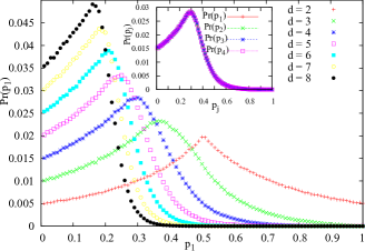
Figure 1: (color online) Probability distribution for the first component of the unbiased probability vector $\mathbf{p}=(p_{1},\cdots,p_{d})$ for one million random samples generated using the iid method. In the inset is shown the probability distribution for the components of the probability vector $\mathbf{p}=(p_{1},p_{2},p_{3},p_{4})$.

Nevertheless, we should note that the sum $\sum_{k=1}^{d}x_{k}$ shall be typically greater than one. This in turn will lead to the impossibility for the occurrence of pRPVs with one of its components equal (or even close) to one. As can be seem in Fig. 1, this problem becomes more and more important as $d$ increases. Therefore, this kind of drawback totally precludes the applicability of the iid method for the task regarded in this article.

4 The normalization method

Lets us begin our discussion of this method by considering a probability vector with dimension $d=2$, i.e., $\mathbf{p}=(p_{1},p_{2})$. If the pRNG is used to obtain $p_{1}\in[0,1]$ and we impose the normalization to get $p_{2}=1-p_{1}$, we are guaranteed to generate an uniform distribution for $p_{j}\in[0,1]$ for both $j=1$ and $j=2$.

If $d=3$ then $\mathbf{p}=(p_{1},p_{2},p_{3})$ and the pRNG is used again (two times) to obtain $p_{1}\in[0,1]$ and $p_{2}\in[0,1-p_{1}]$. Note that the interval for $p_{2}$ was changed because of the normalization of the probability distribution, which is also used to write $p_{3}=1-(p_{1}+p_{2})$. As $p_{1}$ is equiprobable in $[0,1]$, for a large number of samples of the pRPV, its mean value will be $1/2$. This shall restrict the values of the other components of $\mathbf{p}$, shifting the “center” of their probability distributions to $1/4$, biasing thus the pRPV. Of course, if one increases the dimension of the pRPV, the same effect continues to be observed, as is illustrated in the table below for $10^{6}$ pRPV generated for each value of $d$.

$d$	$\langle p_{1}\rangle$	$\langle p_{2}\rangle$	$\langle p_{3}\rangle$	$\langle p_{4}\rangle$	$\langle p_{5}\rangle$
$2$	$0.5001$	$0.4999$
$3$	$0.5000$	$0.2499$	$0.2501$
$4$	$0.4999$	$0.2503$	$0.1248$	$0.1250$
$5$	$0.4998$	$0.2501$	$0.1252$	$0.0625$	$0.0624$

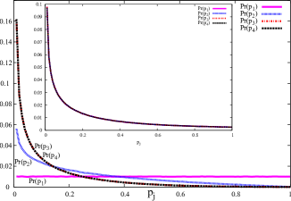
Figure 2: (color online) Probability distribution for the components of the biased probability vector $\mathbf{p}=(p_{1},p_{2},p_{3},p_{4})$ for one million random samples of it. In the inset is shown the probability distribution for the components of the unbiased probability vector $\mathbf{q}=(q_{1},q_{2},q_{3},q_{4})$.

The probability distributions for the four components of the probability vector $\mathbf{p}=(p_{1},p_{2},p_{3},p_{4})$ are shown in Fig. 2. For the sake of illustration, the spaces for the pRPV are sketched geometrically in Fig. 3 for the cases $d=2$ and $d=3$. We observe that the procedure for generating $\mathbf{p}$ as explained above is the motivation for the name of the method, the normalization method.

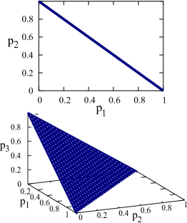
Figure 3: (color online) In blue is shown the set of possible values for the components of the probability vector in the cases of $d=2$ (figure on the top) and for $d=3$ (figure on the bottom). For higher dimensions the probability space is a hyperplane.

A simple solution for the biasing problem just discussed is shuffling the components of the pRPV in each run of the numerical experiment. This can be done, for example, by generating a random permutation of $\{1,2,\cdots,d-1,d\}$, let us call it $\{k_{1},k_{2},\cdots,k_{d-1},k_{d}\}$, and defining a new pRPV as

$$\vec{q} = (q_{1},q_{2},\cdots,q_{d-1},q_{d})$$ (5)

$$:= (p_{k_{1}},p_{k_{2}},\cdots,p_{k_{d-1}},p_{k_{d}}).$$

In the table below is presented the mean value of the components of $\mathbf{q}$ for $10^{6}$ pRPV generated.

$d$	$\langle q_{1}\rangle$	$\langle q_{2}\rangle$	$\langle q_{3}\rangle$	$\langle q_{4}\rangle$	$\langle q_{5}\rangle$
$2$	$0.5005$	$0.4995$
$3$	$0.3332$	$0.3331$	$0.3337$
$4$	$0.2494$	$0.2503$	$0.2499$	$0.2504$
$5$	$0.2001$	$0.1997$	$0.2006$	$0.1999$	$0.1997$

In the inset of Fig. 2 is shown an example with the resulting probability distributions for the four components of $\mathbf{q}=(q_{1},q_{2},q_{3},q_{4})$.

From the discussion above we see that in addition to the $d-1$ pRN needed for the biased pRPV, we have to generate more $d-1$ pRN for the shuffling used in order to obtain an unbiased pRPV (because $\sum_{j=1}^{d}j=d(d+1)/2$), resulting in a total of $2(d-1)$ pRN per pRPV.

5 The trigonometric method

As the name indicates, this method uses a trigonometric parametrization Vedral_Prob_trigo ; Fritzche4 for the components of the probability vector $\vec{p}=(p_{1},\cdots,p_{d})$:

$$p_{j}:=\sin^{2}\theta_{j-1}\prod_{k=j}^{d-1}\cos^{2}\theta_{k},$$ (6)

with $\theta_{0}=\pi/2$ (so the name trigonometric method). More explicitly,

$$p_{1}=\sin^{2}\theta_{0}\cos^{2}\theta_{1}\cos^{2}\theta_{2}\cos^{2}\theta_{3}\cdots\cos^{2}\theta_{d-1}$$

$$p_{2}=\sin^{2}\theta_{1}\cos^{2}\theta_{2}\cos^{2}\theta_{3}\cdots\cos^{2}\theta_{d-1}$$

$$p_{3}=\sin^{2}\theta_{2}\cos^{2}\theta_{3}\cos^{2}\theta_{4}\cdots\cos^{2}\theta_{d-1}$$

$$\vdots$$

$$p_{d-1}=\sin^{2}\theta_{d-2}\cos^{2}\theta_{d-1}$$

$$p_{d}=\sin^{2}\theta_{d-1}.$$ (7)

A simple application of the equality $\cos^{2}\theta_{j}+\sin^{2}\theta_{j}=1$ to this last equation shows that $p_{j}\geq 0$ and $\sum_{j=1}^{d}p_{j}=1$. Therefore this parametrization, which utilizes $d-1$ angles $\theta_{j}$, leads to a well defined probability distribution $\{p_{j}\}_{j=1}^{d}$.

Let us regard the numerical generation of an unbiased pseudo-random probability vector by starting with the parametrization in Eq. (6). Of course, this task is accomplished if the components of the pRPV are created with uniform probability distributions. Thus we can proceed as follows. We begin with $p_{d}$ and go all the way to $p_{1}$ imposing that each $p_{j}$ must be uniformly distributed in $[0,1]$. Thus we must have

$$\theta_{d-1}=\arcsin\sqrt{t_{d-1}}$$ (8)

and the other angles $\theta_{j}$, with $j=1,\cdots,d-2$, should be generated as shown in the next equation:

$$\theta_{j}=\arcsin\sqrt{\frac{t_{j}}{\prod_{k=j+1}^{d-1}\cos^{2}\theta_{k}}},$$ (9)

where $t_{j}$, with $j=1,\cdots,d-1$, are pseudo-random numbers with uniform distribution in the interval $[0,1]$. For obvious reasons, this manner of generating a pRPV is very unstable, and therefore inappropriate, for numerical implementations.

A possible way out of this nuisance is simply to ignore the squared cosines in the denominator of Eq. (9). That is to say, we may generate the angles using e.g.

$$\theta_{j}=\arccos\sqrt{t_{j}}$$ (10)

for all $j=1,\cdots,d-1$. This procedure will give us an uniform distribution for $\cos^{2}\theta_{j}$ and $\sin^{2}\theta_{j}$, but will also increase the chance for the components $p_{j}$ with more terms to have values closer to zero. Thus, there is the issue of a biased pRPV again. A possible solution for this problem is, once more, shuffling. In the next two tables are shown the average value of the components of $10^{6}$ pRPV generated via the trigonometric method before, $\langle p_{j}\rangle$, and after, $\langle q_{j}\rangle$, shuffling.

$d$	$\langle p_{1}\rangle$	$\langle p_{2}\rangle$	$\langle p_{3}\rangle$	$\langle p_{4}\rangle$	$\langle p_{5}\rangle$
$2$	$0.4999$	$0.5001$
$3$	$0.2502$	$0.2498$	$0.4999$
$4$	$0.1250$	$0.1251$	$0.2497$	$0.5003$
$5$	$0.0625$	$0.0624$	$0.1250$	$0.2496$	$0.5006$

$d$	$\langle q_{1}\rangle$	$\langle q_{2}\rangle$	$\langle q_{3}\rangle$	$\langle q_{4}\rangle$	$\langle q_{5}\rangle$
$2$	$0.5006$	$0.4994$
$3$	$0.3331$	$0.3334$	$0.3337$
$4$	$0.2502$	$0.2497$	$0.2501$	$0.2450$
$5$	$0.2005$	$0.1998$	$0.1999$	$0.2001$	$0.1997$

As was the case with the normalization method, for the trigonometric method we need to generate $2(d-1)$ pRN per pRPV, $d-1$ for the angles and $d-1$ for the random permutation. Nevertheless, because of the additional multiplications in Eq. (6), the computation time for the last method is in general a little greater than that for the former, as is shown in Fig. 4.

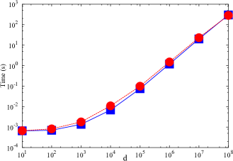
Figure 4: (color online) Log-log plot of the computation time required by the trigonometric method (blue squares) and by the normalization method (red circles) to generate a pseudo-random probability vector with dimension equal to $d$. The calculations were realized using a Processor 1.3 GHz Intel Core i5.

One may wonder if the normalization and trigonometric methods, that are at first sight distinct, lead to the same probability distributions for the pRPV’s components and also if they produce an uniform distribution for the generated points in the probability hyperplane. We provide some evidences for positive answers for both questions in Figs. 5 and 6, respectively.

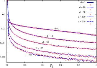
Figure 5: (color online) Semi-log plot of the probability distributions for a component of the unbiased probability vectors generated using the trigonometric (lines) and normalization (points) methods for some values of $d$. We see that the two methods yield, for all practical purposes, the same probability distributions for the components of the pRPV.

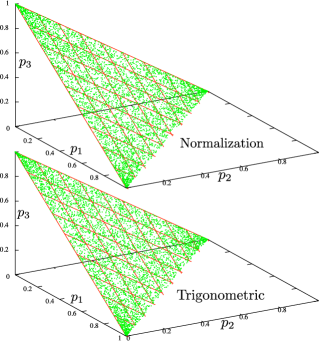
Figure 6: (color online) Sample with five thousand pRPV generated using the indicated method. We see that, in this case for which $d=3$, with exception of the slight overpopulated corners, we get a fairly uniform distribution of points in the probability space.

6 Concluding remarks

In this article we discussed thoroughly three methods for generating pseudo-random discrete probability distributions. We showed that the iid method is not a suitable choice for the problem studied here and identified some difficulties for the numerical implementation of the trigonometric method. The fact that in a direct application of both the normalization and trigonometric methods one shall generate biased probability vectors was emphasized. Then the shuffling of the pseudo-random probability vector components was shown to solve this problem at the cost of the generation of additional $d-1$ pseudo-random numbers for each pRPV.

It is worthwhile recalling that pure quantum states in $\mathbb{C}^{d}$ can be written in terms of the computational basis $\{|c_{j}\rangle\}_{j=1}^{d}$ as follows:

$$|\psi\rangle=\textstyle{\sum_{j}}c_{j}|c_{j}\rangle=\sum_{j}|c_{j}|\mathrm{e}^{\phi_{j}}|c_{j}\rangle=\sum_{j}\sqrt{p_{j}}\mathrm{e}^{\phi_{j}}|c_{j}\rangle,$$ (11)

where $c_{j}\in\mathbb{C}$ and $\phi_{j}\in\mathbb{R}$. The normalization of $|\psi\rangle$ implies that the set $\{p_{j}\}$ is a probability distribution. Thus the results reported in this article are seem to have a rather direct application for the generation of unbiased pseudo-random state vectors.

We observe however that the content presented in this article can be useful not only for the generation of pseudo-random quantum states in quantum information science, but also for stochastic numerical simulations in other areas of science. An interesting problem for future investigations is with regard to the possibility of decreasing the number of pRN, and thus the computer time, required for generating an unbiased pRPV.

- (1) D.J. Bennett, Randomness (Harvard University Press, Massachusetts, 1998)
- (2) L. Mlodinow, The Drunkard’s Walk: How Randomness Rules Our Lives (Pantheon Books, New York, 2008)
- (3) M. Bell, K. Gottfried, M. Veltman, John Bell on The Foundations of Quantum Mechanics (World Scientific, Singapore, 2001)
- (4) M.H. DeGroot, Probability and Statistics (Addison-Wesley, Massachusetts, 1975)
- (5) E.T. Jaynes, Probability Theory: The Logic of Science (Cambridge University Press, New York, 2003)
- (6) D.P. Landau, K. Binder, A Guide to Monte Carlo Simulations in Statistical Physics (Cambridge University Press, Cambridge, 2009)
- (7) T.M. Cover, J.A. Thomas, Elements of Information Theory (John Wiley & Sons, New Jersey, 2006)
- (8) M.A. Carlton, J.L. Devore, Probability with Applications in Engineering, Science, and Technology (Springer, New York, 2014)
- (9) H.V. Ribeiro, E.K. Lenzi, R.S. Mendes, G.A. Mendes, L.R. da Silva, Symbolic sequences and Tsallis entropy, Braz. J. Phys. 39, 444 (2009)
- (10) Á.L. Rodrigues, M.J. de Oliveira, Continuous time stochastic models for vehicular traffic on highways, Braz. J. Phys. 34, 1 (2004)
- (11) F.J. Resende, B.V. Costa, Using random number generators in Monte Carlo simulations, Phys. Rev. E 58, 5183 (1998)
- (12) K.C. Mundim, D.E. Ellis, Stochastic classical molecular dynamics coupled to functional density theory: Applications to large molecular systems, Braz. J. Phys. 29, 199 (1999)
- (13) M.A. Nielsen, I.L. Chuang, Quantum Computation and Quantum Information (Cambridge University Press, Cambridge, 2000)
- (14) M.M. Wilde, Quantum Information Theory (Cambridge University Press, Cambridge, 2013)
- (15) J. Maziero, R. Auccaise, L.C. Celeri, D.O. Soares-Pinto, E.R. deAzevedo, T.J. Bonagamba, R.S. Sarthour, I.S. Oliveira, R.M. Serra, Quantum discord in nuclear magnetic resonance systems at room temperature, Braz. J. Phys. 43, 86 (2013)
- (16) A. Peres, Quantum Theory: Concepts and Methods (Kluwer Academic Publishers, New York, 2002)
- (17) J.J. Sakurai, J. Napolitano, Modern Quantum Mechanics, 2nd Ed. (Pearson Education, San Francisco, 2011)
- (18) J. Grondalski, D.M. Etlinger, D.F.V. James, The fully entangled fraction as an inclusive measure of entanglement applications, Phys. Lett. A 300, 573 (2002)
- (19) R.V. Ramos, Numerical algorithms for use in quantum information, J. Comput. Phys. 192, 95 (2003)
- (20) D. Girolami, G. Adesso, Observable measure of bipartite quantum correlations, Phys. Rev. Lett 108, 150403 (2012)
- (21) D. Girolami, G. Adesso, Quantum discord for general two-qubit states: Analytical progress, Phys. Rev. A 83, 052108 (2011)
- (22) J. Batle, M. Casas, A.R. Plastino, A. Plastino, Entanglement, mixedness, and q-entropies, Phys. Lett. A 296, 251 (2002)
- (23) J. Batle, A.R. Plastino, M. Casas, A. Plastino, On the entanglement properties of two-rebits systems, Phys. Lett. A 298, 301 (2002)
- (24) J. Batle, M. Casas, A. Plastino, A.R. Plastino, Maximally entangled mixed states and conditional entropies, Phys. Rev. A 71, 024301 (2005)
- (25) M. Roncaglia, A. Montorsi, M. Genovese, Bipartite entanglement of quantum states in a pair basis, Phys. Rev. A 90, 062303 (2014)
- (26) S. Vinjanampathy, A.R.P. Rau, Quantum discord for qubit–qudit systems, J. Phys. A: Math. Theor. 45, 095303 (2012)
- (27) X.-M. Lu, J. Ma, Z. Xi, X. Wang, Optimal measurements to access classical correlations of two-qubit states, Phys. Rev. A 83, 012327 (2011)
- (28) F. M. Miatto, K. Piché, T. Brougham, R.W. Boyd, Recovering full coherence in a qubit by measuring half of its environment, arXiv:1502.07030
- (29) J. Shang, Y.-L. Seah, H.K. Ng, D. J. Nott, B.-G. Englert, Monte Carlo sampling from the quantum state space. I, New J. Phys. 17, 043017 (2015)
- (30) Y.-L. Seah, J. Shang, H.K. Ng, D. J. Nott, B.-G. Englert, Monte Carlo sampling from the quantum state space. II, New J. Phys. 17, 043018 (2015)
- (31) G.W. Stewart, The efficient generation of random orthogonal matrices with an application to condition estimators, SIAM J. Numer. Anal. 17, 403 (1980)
- (32) K. Życzkowski, M. Kuś, Random unitary matrices, J. Phys. A: Math. Gen. 27, 4235 (1994)
- (33) E. Brüning, H. Mäkelä, A. Messina, F. Petruccione, Parametrizations of density matrices, J. Mod. Opt. 59, 1 (2012)
- (34) J. Emerson. Y.S. Weinstein, M. Saraceno, S. Lloyd, D. G. Cory, Pseudo-random unitary operators for quantum information processing, Science 302, 2098 (2003)
- (35) V. Vedral and M. B. Plenio, Entanglement measures and purification procedures, Phys. Rev. A 57, 1619 (1998)
- (36) K.Życzkowski, P. Horodecki, A. Sanpera, M. Lewenstein, Volume of the set of separable states, Phys. Rev. A 58, 883 (1998)
- (37) T. Radtke, S. Fritzsche, Simulation of n-qubit quantum systems. IV. Parametrizations of quantum states, matrices and probability distributions, Comput. Phys. Comm. 179, 647 (2008)
- (38) M. Matsumoto, T. Nishimura, Mersenne Twister: A 623-dimensionally equidistributed uniform pseudorandom number generator, ACM Trans. Model. Comput. Sim. 8, 3 (1998)
- (39) M. Wahl, M. Leifgen, M. Berlin, T. Röhlicke, H.-J. Rahn, O. Benson, An ultrafast quantum random number generator with provably bounded output bias based on photon arrival time measurements, Appl. Phys. Lett. 98, 171105 (2011)
- (40) J.A. Miszczak, Employing online quantum random number generators for generating truly random quantum states in Mathematica, Comput. Phys. Comm. 184, 257 (2013)