Simulations of reflected radio signals from cosmic ray induced air showers

Abstract

We present the calculation of coherent radio pulses emitted by extensive air showers induced by ultra-high energy cosmic rays accounting for reflection on the Earth’s surface. Results have been obtained with a simulation program that calculates the contributions from shower particles after reflection at a surface plane. The properties of the radiation are discussed in detail emphasizing the effects of reflection. The shape of the frequency spectrum is shown to be closely related to the angle of the observer with respect to shower axis, becoming hardest in the Cherenkov direction. The intensity of the flux at a fixed observation angle is shown to scale with the square of the primary particle energy to very good accuracy indicating the coherent aspect of the emission. The simulation methods of this paper provide the foundations for energy reconstruction of experiments looking at the Earth from balloons and satellites. They can also be used in dedicated studies of existing and future experimental proposals.

1 Introduction

There is a renewed interest in using the radio technique for the detection of extensive air showers induced by Ultra-High Energy Cosmic Rays (UHECR). Dedicated experimental initiatives such as CODALEMA [1], LOFAR [2], AERA [3], LOPES [4] and Tunka-Rex [5], with instrumentation far superior to that used in the early days of radio detection, have stimulated an impressive progress in the field. As a result the possibility of using the radio technique, either as a complement to other techniques for the detection of extensive air showers, or even to design new UHECR detectors based on it, is now seriously considered [6].

The serendipitous discovery of 16 fast radio pulses from air showers extending up to the GHz range with the first ANITA balloon born antenna system [9] came as a surprise. This system, operating with a frequency band between 200 and 1200 MHz, had been originally conceived for detecting radio emission from neutrino interactions in the Antarctic ice sheet. However, the detected emission was strongly polarized in the direction defined by the cross product of the geomagnetic field and the shower direction, which is characteristic of radio signals from air showers due to the current induced by the Earth’s magnetic field [1, 10]. Detailed simulations of these pulses showed recently that coherent emission can extend up to and above GHz frequencies [7, 8] in spite of simple dimensional arguments suggesting the contrary [12]. This is because the varying refractive index of the atmosphere introduces a significant effect on the relative travel time of emissions originating from different locations. When these delays are accounted for, a Cherenkov like ring can appear in which the signals from a large region of the shower arrive with little time delay and thus add coherently [8]. This angle is mostly determined by the refractive index at the shower maximum, simply because that is the region with more charge and current and hence contributing most.

Fourteen out of the sixteen detected pulses were reconstructed to be coming from distinct points on the polar ice cap and showed inverted polarity with respect to the other two. This was interpreted as clear evidence that they were detected after reflection on the polar ice cap. The reflection of the radio flashes introduces several new aspects to the calculation of pulses at the detector that have not been previously addressed. Naturally reflection implies a reduction of the emission due to the Fresnel coefficients. The relative time delays with respect to detection at ground level are also altered, since the pulses propagate upwards after reflection towards the top of the atmosphere along a decreasing refractive index profile. These effects need to be taken into consideration to interpret the events detected by ANITA and to evaluate the acceptance of experiments that rely on observing radiation induced by showers from mountain tops, balloon payloads [13] such as the next ANITA flight and EVA [14] or from satellite payloads as proposed in SWORD [15].

In this article we simulate and describe the properties of radio pulses emitted from extensive air showers after reflection off a surface. Most of the calculations are performed in a configuration suited for a high altitude balloon flight over Antarctica, however the developed methods can be applied to other reflective surfaces and different detector altitudes. We modified the ZHAireS code [16] to calculate the radio emission from air showers after reflection on a flat surface. We first describe the geometry and explain the assumptions made to adapt the program to calculate the reflected radiation. After this we generate a set of simulations to investigate the signal properties as a function of off-axis angle, frequency, zenith angle, and energy of the primary particle, and stress the importance of properly accounting for the Fresnel coefficients in the reflection, as well as for the propagation of the pulses towards the top of the atmosphere. In the Appendix we use a ray tracing code and a simplified model for the emission (that displays the main features of the predicted radiation as has been justified elsewhere [8, 17]), to confirm that the effect of curved light trajectories can be neglected.

2 Geometry and scales relevant for reflected events

The appealing aspect of observing radiation of air showers after reflection is that a large atmospheric volume can be monitored with a single detector. Therefore, the most interesting geometry is given by air showers that impact Earth’s surface at large zenith angles.

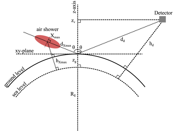
Figure 1: Basic geometry for reflected signals from air showers (see text for details, see also Fig. 2).

The basic geometry of the problem is sketched in Fig. 1. We define a rectangular coordinate system with the $z$-axis pointing upwards in the vertical direction and the $x-y$ plane tangent to the Earth’s surface. The reflective surface will be approximated by this plane. The origin of the coordinate system is the point at which the shower axis intercepts the Earth’s surface which is assumed to be at a ground altitude $z_{g}$ above sea level. The zenith angle of the shower, $\theta$, is defined with respect to the $z-$axis. We define the off-axis angle $\psi$ in Fig. 2, to describe the angular deviation of the emitted radiation with respect to the shower axis. A generic detector is positioned at a point with vertical altitude $h_{d}$. In Fig. 1 the detector is displayed in a special position such that it sees the reflected radiation which was emitted precisely along the direction of shower axis with $\psi=0^{\circ}$. The altitude at which shower maximum ($X_{\rm max}$) is reached, $h_{\rm Xmax}$, is also of relevance. Besides determining the angle at which the emission is largest [8], it also sets the scale of distances the pulse has to travel to reach the detector, $d_{\rm Xmax}+d_{d}$, where $d_{\rm Xmax}$ and $d_{d}$ respectively denote the distances from the origin of the coordinate system to shower maximum and to the detector.

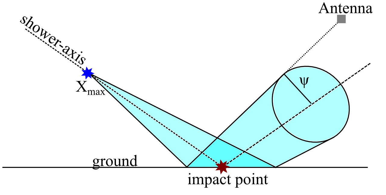
Figure 2: To describe a location of an antenna we use the “off-axis” angle $\psi$, as that between the shower axis and the line joining the location of $X_{\text{max}}$ and the position of the antenna.

We illustrate the typical scales of this geometry by showing in Fig. 3 some parameters for a high altitude balloon over Antarctica. We take a detector at a typical altitude of $h_{d}=35~{}{\rm km}$, a ground altitude of the ice cap of $z_{g}=2~{}{\rm km}$ and the Earth’s radius $R_{E}=6357~{}{\rm km}$. The distance $d_{d}$ becomes simply a function of $\theta$ which is illustrated in the top panel of Fig. 3. To estimate the distance to shower maximum, $d_{\text{Xmax}}$, we use the average slant depth of shower maximum $\langle X_{\text{max}}\rangle$ as observed by the Pierre Auger Observatory [18, 19] together with the atmospheric density profile used in the air shower simulation package AIRES [20]. Clearly the average position of $X_{\rm max}$ depends on shower energy, but the effect is accidentally small according to the measurements at the Pierre Auger Observatory which indicate little change of $X_{\rm max}$ in the energy range of $10^{17.8}$ to $10^{19.6}$ [18, 19]. The results for different primary energies are shown as a function of $\theta$ in the middle panel of Fig. 3. It should be noted that the measured RMS fluctuations of $X_{\rm max}$ are between $20$ and $60$ g cm^-2[18, 19] corresponding to variations of $d_{\rm Xmax}$ below $11\%$ ($3\%$) for a zenith angle of $60^{\circ}$ ($85^{\circ}$) degrees. The variation relative to the total distance travelled by the pulse $d_{\rm Xmax}+d_{d}$ reduces to $1.5\%$ (1.0%).

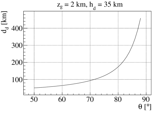
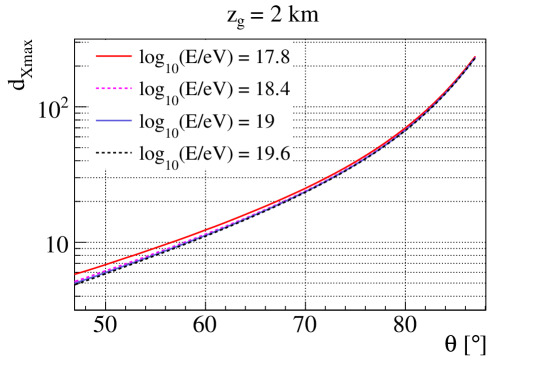
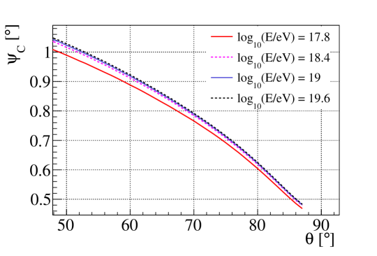
Figure 3: Top panel: distance from the reflection point to the detector ($d_{d}$ in Fig. 1); middel panel: distance to shower maximum ($d_{\rm Xmax}$ in Fig. 1); and bottom panel: the Cherenkov angle at $X_{\text{max}}$ as a function of shower zenith angle. For the location of $X_{\text{max}}$ we used the average value of $\langle X_{\text{max}}\rangle$ as a function of energy as measured by the Pierre Auger Collaboration [18, 19].

A relevant parameter is the Cherenkov angle, $\psi_{C}\approx\cos^{-1}(1/n)$, at the location of $X_{\text{max}}$ that is directly obtained using the refractive index $n$ at the corresponding altitude, $h_{Xmax}$. In the following the refractive index is approximated by a simple exponential function of altitude $h$ given by $n(h)=1+\eta_{0}\,e^{-\kappa h}$, with $\eta_{0}=325\times 10^{-6}$ and $\kappa=0.1218$ km^-1 [16]. The Cherenkov angle at $X_{\text{max}}$ is shown in Fig. 3 (bottom) for the above parameterization.

3 Introducing reflection in ZHAireS

ZHAireS [16] is a simulation program that has been developed combining the AIRES package for air shower simulations [20] with the “ZHS algorithm” which was originally developed to calculate radio emission from high energy showers in homogeneous ice [21, 22] and then extended for use in air showers [16, 23]. The contribution from each track element to the radio pulse at any given position and time is calculated in ZHAireS assuming the particle travels at a constant speed and in a rectilinear motion and also accounting for the travel times taken by the radiation to reach from each of the ends of the track [16, 24]. To calculate travel times in ZHAireS we perform a numerical integration to account for the variation of the index of refraction with altitude assuming that the emission travels in straight lines to the observer (see below). The curvature of the Earth’s atmosphere is fully accounted for in AIRES.

We have modified the ZHAireS code to deal with the reflection of air shower radio emission on a surface. For each rectilinear track element we first find the point on the reflection surface and the angle of emission of radiation with respect to the track so that the emitted ray propagates first to the reflection point and then upwards towards the observer at a fixed position. Approximating the reflection surface to a plane makes it trivial to obtain this reflection point for a ray coming from any point in the atmosphere. Once this is known, the time delay due to the refractive index is easily calculated integrating the travel time over the total path of the ray before and after the reflection. We assume that the emission travels in a straight lines to the observer. We have explored the validity of this approximation using a simple one dimensional model to produce pulses which resemble the fully simulated ones. This model allows the calculation of travel times using numerical methods to propagate signals along curved trajectories. The properties of the pulses obtained with straight ray approximation are equivalent to those accounting for curvature up to shower zenith angles $\theta\sim 85^{\circ}$ and frequencies of $\sim 1$ GHz. This study is described in detail in the Appendix.

As mentioned before, we approximate the reflection surface to the $xy$-plane defined in Section 2, assumed to be perfectly flat. The bulk of the emission has been shown to be concentrated in a cone that makes a small “off-axis” angle $\psi$ to the shower direction as shown in Fig. 2. This angle is very close to the Cherenkov angle ($0.5^{\circ}-1^{\circ}$) at an altitude at which shower maximum occurs [8]. As a consequence the illuminated region on the reflective surface is relatively small, of order $0.5~{}{\rm km}$ $\times$ $1~{}{\rm km}$ ($1.5~{}{\rm km}$ $\times$ $10~{}{\rm km}$) for a $\theta=60^{\circ}$ ($80^{\circ}$) shower. As a result it is reasonable to ignore the differences in the orientation angle and altitude of the reflecting surface at the locations of the different reflection points across the illuminated area. These differences are below $0.1^{\circ}$ and a few meters respectively even for showers of $\theta=80^{\circ}$. There are other important aspects to the flat mirror approximation. When rays are reflected on a convex and rough surface they will diverge after reflection, and therefore the power received at a given surface element will be typically less than when a flat reflector is assumed. These effects have been studied in [15] and [25], and have little impact at moderate zenith angles, however they can become significant for high zenith angles ($\theta>80^{\circ}$). Results of the simulations with the reflective surface assumed flat can be corrected “a posteriori” following the procedures outlined in  [15, 25]. Such calculation is however very detector specific, and out of the scope of this article. Despite this, we expect the simulation method presented in this work to be very suitable for that purpose.

At each reflection point the Fresnel coefficients are applied to the time-domain electric field to calculate the attenuation of the components with polarization parallel, $r_{\mathrm{\|}}$, and perpendicular, $r_{\perp}$, to the reflection plane, defined by the normal to the reflecting surface and the direction of the radiation:

$$r_{\perp}=\frac{n_{1}\cos\theta-n_{2}\sqrt{1-\left(\frac{n_{1}}{n_{2}}\sin\theta\right)^{2}}}{n_{1}\cos\theta+n_{2}\sqrt{1-\left(\frac{n_{1}}{n_{2}}\sin\theta\right)^{2}}},~{}~{}{\rm and}~{}~{}r_{\mathrm{\|}}=\frac{n_{1}\sqrt{1-\left(\frac{n_{1}}{n_{2}}\sin\theta\right)^{2}}-n_{2}\cos\theta}{n_{1}\sqrt{1-\left(\frac{n_{1}}{n_{2}}\sin\theta\right)^{2}}+n_{2}\cos\theta}.$$ (1)

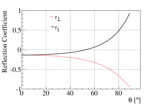
Figure 4: The Fresnel coefficients for an air-ice interface with refractive indices 1.0003 and 1.31 respectively, as a function of the zenith angle $\theta$ of the incident ray.

The Fresnel coefficients for an air-ice interface are shown in Fig. 4 as a function of zenith angle $\theta$ of the incident ray. A large fraction of the components of the field is not reflected below $\theta\sim 70^{\circ}-80^{\circ}$, and in fact at the Brewster angle at $\theta\sim 53^{\circ}$ the parallel component is not reflected at all. The coefficients change rapidly above $\theta\sim 60^{\circ}$. Clearly they have a drastic impact on the the overall amplitude, the polarization and the zenith angle dependence of the radio signal as will be shown in Section 4.

4 Simulations for a high altitude detector

4.1 Simulation set and considerations

In this section we apply the implementation of the reflection in ZHAireS to a configuration that resembles a high altitude balloon experiment over Antarctica, such as the ANITA flights, or the planned EVA mission [14].

We place antennas at a fixed altitude $h_{d}=36~{}{\rm km}$ above sea-level, and choose the reflecting surface to be at $z_{g}=2~{}{\rm km}$ above sea-level. We adopt a refractive index of $n=1.31$ [26] consistent with ANITA measurements of the reflected image of the Sun [27]. The geomagnetic field is chosen to have a typical value of 55 $\mu$T and an inclination of $-70^{\circ}$. We generated proton showers with zenith angles $\theta=\{57^{\circ},64^{\circ},71^{\circ},78^{\circ},85^{\circ}\}$ and azimuth such that they always arrive from the geomagnetic west. For each zenith angle, we generate air showers with energies $E=\{10^{17.8},10^{18.4},10^{19},10^{19.6}\}$ eV. We select simulations that have a $X_{\text{max}}$ similar to the average $\langle X_{\text{max}}\rangle_{\text{Auger}}$ observed at the Pierre Auger Observatory. To do so, we pre-simulate seven air showers per configuration with different random seeds and we select the air shower closest to $\langle X_{\text{max}}\rangle_{\text{Auger}}$. This results in an average deviation of $|X_{\text{max}}-\langle X_{\text{max}}\rangle_{\text{Auger}}|\approx 18$ g cm^-2, which is within the root mean square of the energy-dependent $X_{\text{max}}$-distributions that have been observed. The shower simulation is run with AIRES using QGSJETII.03 hadronic model interactions with a thinning level of $10^{-5}$ [20].

4.2 Results

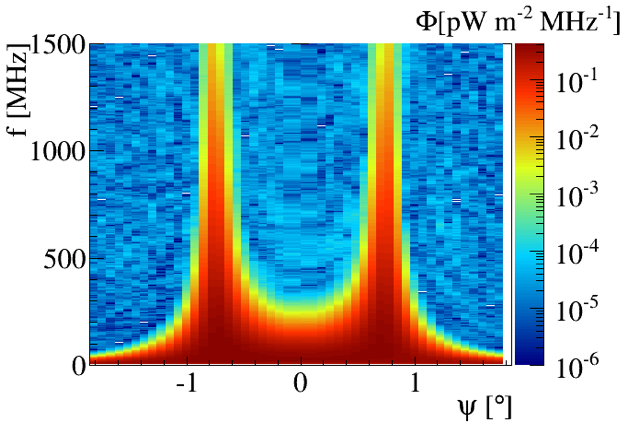
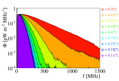
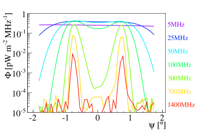
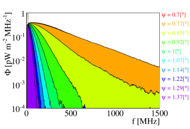
Figure 5: Top left panel: distribution of the radio signal (flux density $\Phi$) as a function of off-axis angle $\psi$ (Fig. 2) and frequency $f$ for an air shower with $\theta=71^{\circ}$ and $\log_{10}(E/\text{eV})=18.4$. In the bottom left panel we show the distribution of the radio signal as a function of off-axis angle at various frequencies. In the right panels we show the radio signal distribution as a function of frequency, in the top right panel for off-axis angles equal or smaller than the Cherenkov-angle at the $X_{\rm max}$ of the shower i.e. $\psi\leq 0.7^{\circ}$, while in the bottom right panel for $\psi\geq 0.7^{\circ}$.

To illustrate some of the typical features of the radio signal, we display in Fig. 5 the flux density $\Phi$ as a function of frequency and off-axis angle $\psi$ for an air shower with zenith angle $\theta=71^{\circ}$ and a energy $E=10^{17.8}$ eV. The flux density in this case is defined as the power spectrum at a fixed frequency $f$ averaged over a period of 10 ns, and is given in units of ${\rm pW~{}m^{-2}~{}MHz^{-1}}$ throughout this paper. In the top left panel of Fig. 5 we show the two-dimensional distribution as a function of $\psi$ and $f$ which displays coherent properties and is clearly beamed around the Cherenkov angle at $\sim 0.77^{\circ}$. This can be better appreciated in the bottom left panel where we show the off-axis distributions for different frequency components of the pulse. As the frequency increases the radiation adds coherently only within a smaller angle off the Cherenkov cone. In the right panels in Fig. 5 we show the spectral shape of the flux density for a variety of observation off-axis angles. At very low frequencies ($f<10~{}{\rm MHz}$) the flux density increases until it reaches a maximum in the range ($f\sim 10-150~{}{\rm MHz}$) and then decreases with an exponential fall-off to first order. A very important feature is illustrated in the right panels, the steepness of the fall-off has a clear dependence on the off-axis angle $\psi$ of the detector. This dependence is key to the energy determination of UHECRs with ANITA as pointed out in [28].

4.2.1 Implications of the reflection

Other efforts to simulate reflected radio signals from air showers have relied on pulses simulated at ground which were extrapolated using the attenuation of the signal with increased distance ($|\vec{E}|\propto 1/r$) after accounting for the loss of signal induced by the Fresnel coefficients [28]. In a homogeneous medium this “specular approach” can be expected to be a good approximation provided the pulse can be considered to be in the Fraunhofer limit. As a result it can be expected to work better for highly inclined showers, since the distance between the observer and air shower increases as the zenith angle rises.

In this work all track contributions to the pulse are reflected at the interface to account for attenuation with distance, for the Fresnel-reflection coefficents attenuating the parallel and perpendicular components of the field, and for the fact that reflection also alters the relative time delays of emission from different regions of the shower affecting the coherence properties of the pulses. Therefore, this method can also be applied when the reflector is not in the Fraunhofer limit.

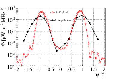
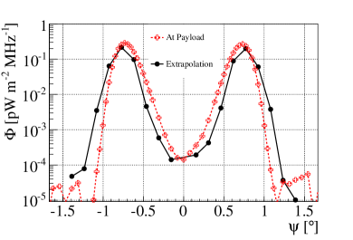
Figure 6: Flux density $\Phi$ at a frequency $f=300~{}{\rm MHz}$ as a function of off-axis angle $\psi$ as obtained extrapolating the ZHAireS simulated signal at ground to the detector (black dots and solid line), and simulating the reflection as explained in the text (red crosses and dashed line). The flux density is shown for showers of $E=10^{18.4}$ eV and two zenith angles $\theta=57^{\circ}$ (left panel) and $\theta=71^{\circ}$ (right panel). The Fresnel-reflection coefficients are accounted for in all cases.

We compare the specular approximation to the results of the full ZHAireS simulation including reflection to illustrate the difference between the two methods. For this comparison we evaluate the flux density at $f=300~{}{\rm MHz}$ at a few ground locations scaling it to account for the distance from ground to the location of the high altitude balloon. In Fig. 6 we display the flux density as a function of $\psi$ for two different zenith angles. We note that for $\theta=57^{\circ}$ (Fig. 6 left) the distribution in $\psi$ is significantly wider what can lead to orders of magnitude of over-estimation of the flux density for the larger off-axis angles. For $\theta=71^{\circ}$ (Fig. 6 right) we still see relevant deviations between the two methods, but they are significantly reduced compared to the lower zenith angle case. Significant deviations are also found at other frequencies. Moreover, the shapes of the frequency spectra obtained with the two methods also differ appreciably.

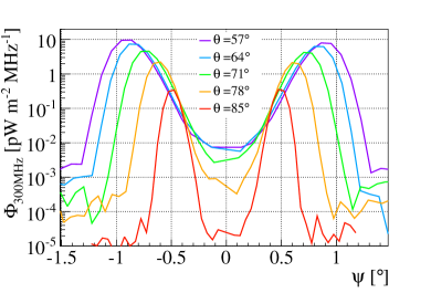
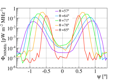
Figure 7: Comparison of the flux density $\Phi$ at a frequency $f=300~{}{\rm MHz}$ as a function of the off-axis angle $\psi$ before (left) and after applying Fresnel reflection coefficients (right). Different sets of curves correspond to different shower zenith angles $\theta$ as labeled. The simulated showers have an energy $E=10^{18.4}$ eV.

It is interesting to explore how the radiation changes with zenith angle for a primary particle with fixed energy. As the zenith angle increases the flux density $\Phi$ decreases. This can be seen in the left panel of Fig. 7, displaying $\Phi$ at $f=300~{}{\rm MHz}$ as a function of $\psi$ for an air shower induced by a primary particle with energy $E=10^{18.4}$ eV. The dominant effect in the decrease is the increasing overall distance to the detector with $\theta$ (see Fig. 3). Other effects however compensate the decrease in $\Phi$. The angle $\alpha$ of the shower axis to the Earth’s magnetic field at the South Pole increases in the range of $\theta$ shown in Fig. 7, and the geomagnetic contribution is known to scale with $\sin\alpha$. Also showers of increasing $\theta$ develop in a less dense atmosphere where the geomagnetic contribution to the electric field is expected to be increasingly larger [30]. The net result, including other more subtle effects [29], is a decrease of $\Phi$ with $\theta$.

To illustrate the importance of accounting for the Fresnel reflection coefficients they were artificially set to 1 in the simulations shown in the left panel of Fig. 7, while in the right panel they are taken into account. Comparing both panels, the peak value of the flux density is largest at relatively high zenith angles ($\theta\sim 80^{\circ}$) when the Fresnel coefficients are accounted for, contrary to what is seen in the left panel where the peak value of $\Phi$ is achieved at the smallest zenith angles. This suggests that detection can be expected to be most favorable for $\theta$ around $80^{\circ}$. A thorough calculation of the acceptance integrating over area and solid angle [13] should also account for the reduction of the Cherenkov angle as the zenith angle rises (see Fig. 3), and for the directionality of the detection system. Such calculation is out of the scope of this article.

4.2.2 Energy dependence

From the set of simulations we have examined the energy dependence of the radio signal. As before, we use the flux density at a reference frequency $f=300~{}{\rm MHz}$ for a shower of $\theta=71^{\circ}$.

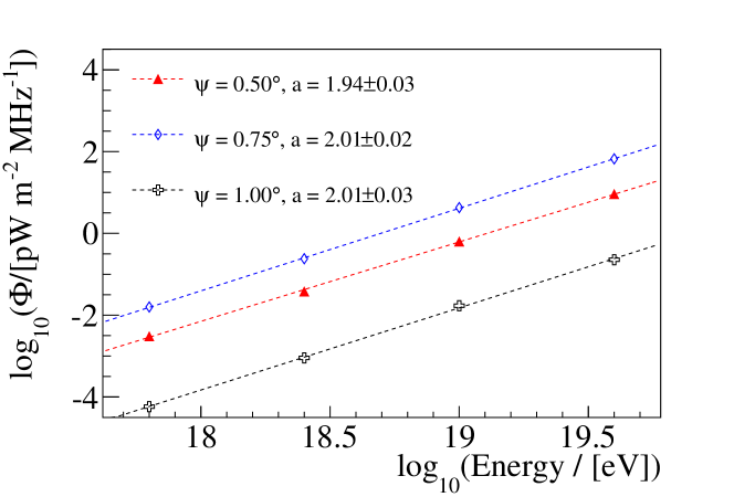
Figure 8: The flux density $\Phi$ at frequency $f=$300 MHz as a function of the energy of the primary particle for three off-axis angles in a shower of $\theta=71^{\circ}$. The results of fitting a straight line $\log_{10}\Phi=a\log_{10}(E/\text{eV})+b$ are shown.

In Fig. 8 we select three off-axis angles and plot the flux density as a function of the primary particle energy. We fit a simple linear function to the dependence of $\log_{10}\Phi$ on $\log_{10}(E)$ and find a slope that is consistent with 2. This confirms that the received flux density scales quadratically with the primary energy and the amplitude of the electric field scales linearly with it. This is not surprising since for a coherent signal it is expected that the amplitude of the electric field scales with the number of electrons in the shower which is proportional to the energy of the primary particle. We verified that the quadratic relation between flux density and energy of primary cosmic ray particle holds for all the zenith angles and all considered frequencies in our simulation set. This has important consequences since measuring the flux density at a given off-axis angle provides a measurement of the energy of the air shower. In practice the off-axis angle can be related to the exponential fall-off of the flux density as can be seen in Fig. 5. This relation is key to the energy determination of UHECRs with ANITA [28]. This means that it is in principle possible to deduce the primary energy from a single location as long as the exponential fall-off of the spectrum can be determined.

5 Conclusions

In this paper we implemented the treatment of surface reflection for radio signals from air showers, upgrading existing ZHAireS simulations.

As a case study we simulated radiation from a set of air showers at a high altitude position over Antarctica inspired by the ANITA experiment which has provided the only measurements of reflected radio pulses from air showers up to now. We described and explained the flux density distributions as a function of frequency, energy and zenith angle of the primary cosmic ray particle. We have stressed the importance of accounting for the Fresnel-reflection coefficients attenuating the components of the field, as well as accounting for the fact that reflection also alters the relative time delays of emission from different regions of the shower affecting the coherence properties of the pulses.

A clear quadratic correlation between the radio observable (flux density) and the shower energy has been observed in ZHAireS simulations with reflection. The intercept of the correlation depends on the off-axis angle which can be related to the exponential fall-off of the spectral distribution of the flux density. This provides the basis for the determination of shower energy from a single location [28].

Several approximations were made in the implementation of the reflection in the ZHAireS code. The reflective surface is assumed to be a plane and we argued that this is a good approximation as long as the shower zenith angle is $\theta\lesssim 80^{\circ}$. Also the emitted radiation is assumed to travel along straight lines to the ground and then to the detector, an approximation that has been extensively verified in Appendix A.

Finally, we foresee many applications of this code to the design and feasibility studies of future large exposure cosmic ray detectors based on the radio technique applied to air showers [15, 13].

Appendix A Appendix

A.1 Straight vs curved ray propagation

The variation with altitude of the index of refraction of the atmosphere is known to induce curvature in the path of the radio waves when propagating. It has been shown that the effects are negligible for most shower geometries and observers on ground [31], for which the propagation along straight paths is a good approximation. In the case of showers at large zenith angles and especially when accounting for reflection, the involved distances from emission to the detector become large (see Figs. 1 and 3), and the curvature of the rays can be expected to increase.

To evaluate if the approximation of straight light ray propagation still holds in the typical geometries involved in reflection, we have developed a simple ray tracing code. We divide the atmosphere in many layers with constant distance between them. The layers are taken sufficiently narrow so that the ray can be approximated as traveling in a straight line along a constant refractive index $n$ in each layer given by the exponential model in Section 2. The ray is refracted at each interface, taking into account the different refractive index at each layer. The travel time of the ray is calculated as the sum of the times it takes to cross each layer. When accounting for reflection on the ground, the ray is also propagated upwards through a decreasing refractive index profile until it reaches the detector. The arrival time assuming straight line propagation to ground and then to the same detector position is also calculated. The reflection surface is assumed to be at sea level for these calculations. Since the gradient of an exponential atmosphere is largest at sea level, it can be expected that curvature effects for reflection from surfaces at higher altitudes will have less impact than estimated here.

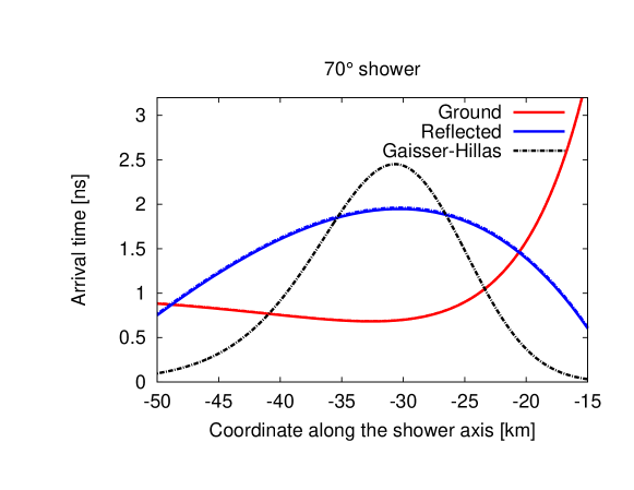
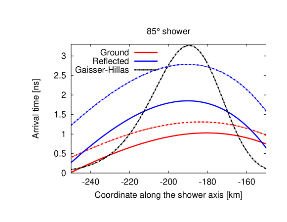
Figure 9: Top: Relative arrival time of rays emitted along the axis of a $\theta=70^{\circ}$ shower at two particular antenna locations: one located on the ground (red lines) and another after reflection towards a high altitude balloon (blue lines) both at an off-axis angle close to the Cherenkov angle $\psi\sim 0.77^{\circ}$ (see Fig. 2). The straight ray approximation (dashed lines) and the curved ray propagation (solid lines) are shown (see text for details). A $10^{19}$ eV, $\theta=70^{\circ}$ Gaisser-Hillas shower profile is superimposed (black line). Bottom: the same as in the top panel, but now for a $\theta=85^{\circ}$ shower viewed at an off-axis angle $\psi\sim 0.40^{\circ}$.

In Fig. 9 (top panel) we show the relative arrival times of radio signals emitted from different positions along the shower axis of a $\theta=70^{\circ}$ shower. They have been calculated with the straight and curved ray approximations for two particular observer positions such that the radiation arriving from shower maximum makes an off-axis angle $\psi\sim 0.77^{\circ}$. One observer is located on the ground and receives the rays directly, the other observer is placed at an altitude $h_{d}\simeq 33~{}{\rm km}$ and receives the rays after reflection on the ground (see Fig. 1). The difference in the arrival times between curved and straight ray propagation is hardly noticeable in the scale of Fig. 9. It is in fact below $\sim 50$ ps, which corresponds to a frequency of $\sim 5$ GHz when using a quarter wavelength criterion for coherence. As a result we expect the straight ray approximation to be valid below this frequency.

Similarly in Fig. 9 (bottom panel) we show the arrival times of the pulses for a $\theta=85^{\circ}$ shower and observation at an off-axis angle $\psi=0.4^{\circ}$. Although in this case the difference between curved and straight ray propagation is sizable, it is an almost constant offset along shower development of $\sim 0.3$ ns for the observer on the ground and $\sim 0.9$ ns for the observer at high altitude $h_{d}=50~{}{\rm km}$. This global offsets induce unobservable phase shifts in the field at the detector. When accounting for these offsets, the relative differences between the straight and curved propagations are $\sim 200$ ps for the observer at ground level corresponding to a frequency of $\sim 1.25$ GHz using a quarter wavelength criterion, while for the observer at $h_{d}=50~{}{\rm km}$ altitude the differences are below $\sim 20$ ps ($\sim 12$ GHz frequency).

In the top and bottom panels of Fig. 9 the relative arrival times at ground and at the high altitude observer are approximately flat within a large region ($\sim 10~{}{\rm km}$) around shower maximum. As a result the emission from this region is coherent up to GHz frequencies. An interesting feature in the top panel of Fig. 9 is the inversion of the arrival times at the high altitude observer position. The radio signal emitted in the Cherenkov angle (in this particular case from the region around shower maximum) arrives last at the high altitude location, contrary to what could be expected in a homogeneous medium. The time inversion is also seen for the observer on the ground for the $85^{\circ}$ shower in Fig. 9 (bottom). The effect does not seem to have relevant implications for detection.

A.2 A simple model to describe the pulses

The comparison of the travel times for the straight and curved ray calculations already sheds light onto the validity of the straight ray approximation. However a comparison between the pulses obtained with the straight and curved approaches in a simplified calculation will give us an estimate of the quantitative uncertainty in the properties of the signal at the detector when using the straight path approximation.

For that purpose, we model a shower with zenith angle $\theta$ as a one-dimensional charge distribution varying with time $N(t)$ as the shower propagates along a given direction at the speed of light $c$ [17]. In the Fraunhofer approximation [23], the electric field induced by this line of charge is proportional to the charge $N(t)$, to $r^{-1}(t)$, with $r(t)$ the distance between the emission point and the observer position, and carries a phase factor to account for the time delay between the arrival of the signal emitted from different positions along the line:

$$E\sim\int\mathrm{d}t\ N(t)\frac{e^{i\omega t_{a}(t)}}{r(t)}$$ (2)

Here $\omega$ is the angular frequency and $t_{a}$ is the arrival time at the observer of a signal emitted at time $t$, where

$$t_{a}(t)=t+\frac{n}{c}~{}r(t)$$ (3)

This approximation was developed for a homogeneous, isotropic and non-conductive medium but it can be extended to the atmosphere accounting for the time delays from propagation of the rays in the altitude-dependent index of refraction [16].

In Fig. 10 the pulses obtained in the full ZHAireS simulation modified for reflection are compared to those obtained with Eq. (2) using as input a one-dimensional Gaisser-Hillas distribution, $N(t)$, with the same depth of shower maximum as the simulated shower. The amplitude of the reflected field is shown for observers at a high altitude located at different off-axis angles $\psi$ (see Fig. 2) and constant overall path distance. The results have been normalized to the peak of the electric field as predicted with Eq. (2). The shape of the angular distribution is well described by the simple model in a wide frequency range. It should be noted here that, being one-dimensional, the approach can not fully reproduce the frequency spectrum as obtained in the full simulations near the Cherenkov angle, where the lateral spread is of utmost importance [16]. We are however confident that the approximation is sufficient to test the validity of the straight ray approximation.

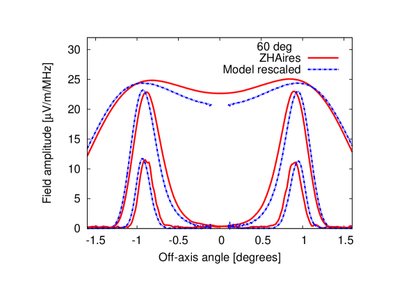
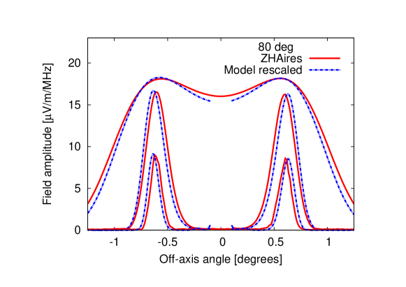
Figure 10: Top: amplitude of the Fourier transformed electric field as a function of the off-axis angle for different frequencies. Results from full ZHAireS simulations and the model in Eq. (2) are shown. The shower has $E=10^{19}$ eV, $\theta=60^{\circ}$ and a height of $X_{\rm max}$ above ground $h_{\rm Xmax}\sim 4.4~{}{\rm km}$. The observers are placed at a constant distance from $X_{\rm max}$ of $\sim 83.3~{}{\rm km}$. From top to bottom the observation frequencies are $50$, $300$ and $900~{}{\rm MHz}$. Bottom: Same as in the top panel, but for a $\theta=80^{\circ}$ shower with $h_{\rm Xmax}\sim 13.5~{}{\rm km}$ and with the observers placed at a constant distance of $\sim 276.9~{}{\rm km}$.

A.3 Validity of the straight ray approximation

We used the simplified one-dimensional model described above to test the straight ray approximation. The arrival times $t_{a}$ at the detector to be used in Eq. (2) are calculated integrating the travel time along both straight and curved paths using the ray tracing algorithm explained above. The electric field is obtained numerically, discretizing the integral in Eq. (2) in such a way that the time intervals correspond to regions of the shower with approximately constant $N(t)$, $r(t)$ and $t_{a}(t)$.

The results using the straight and curved ray calculations are compared in Fig. 11 where we plot the modulus of the electric field as a function of the offset angle of the antenna $\psi$ for showers of $\theta=70^{\circ}$ (top) and $\theta=85^{\circ}$ (bottom). As anticipated from arguments concerning the travel times discussed at the beginning of this Appendix, the difference in the angular distribution of the electric field between the straight and curved ray propagation is negligible for the $\theta=70^{\circ}$ shower at all the frequencies we probed. It can be appreciated that even for $\theta=85^{\circ}$, the effect is still negligible up to a frequency of $900~{}{\rm MHz}$. This justifies the straight ray approximation for the calculation of the angular distribution of the field, even at high zenith angles and up to GHz frequencies.

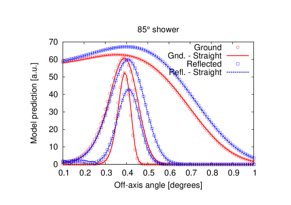
Figure 11: Top: Electric field modulus as obtained with the simple model in Eq. (2), as a function of the off-axis angle $\psi$ for three frequencies. The observers are located at different $\psi$ angles on the ground (red solid lines) and at an overall distance $\sim 130~{}{\rm km}$ to $X_{\rm max}$ after reflection (blue dashed lines). The shower has $\theta=70^{\circ}$ and $X_{\rm max}$ at an altitude above ground $h_{\rm Xmax}\sim 10.4~{}{\rm km}$. The results of curved (points) and straight (lines) rays calculation are shown. From top to bottom, the observation frequencies are $50$, $300$ and $900~{}{\rm MHz}$. Bottom: the same as in the top panel with the observers located on the ground and at an overall path distance of $\sim 648.5~{}{\rm km}$. The shower has $\theta=85^{\circ}$ and $h_{\rm Xmax}\sim 16.5~{}{\rm km}$. In both panels the fields on the ground are rescaled with the corresponding ratio of the distance to the ground and the total distance to the detector for visibility.

References

- [1] D. Ardouin et al. [CODALEMA Collaboration], Astropart. Phys. 31 (2009) 192.
- [2] P. Schellart et al. [LOFAR Collaboration], Astron. & Astrophys. 560 (2013) A98.
- [3] F.G. Schröder for the Pierre Auger Collaboration, Proceedings of the ICRC, Rio de Janeiro, Brazil (2013), #0899.
- [4] H. Falcke et al. [LOPES Collaboration], Nature 435 (2005) 313.
- [5] F.G. Schröder for the Tunka-Rex Collaboration, Proceedings of the ICRC, Rio de Janeiro, Brazil (2013), #0452.
- [6] T. Huege, Proceedings of the ICRC, Rio de Janeiro, Brazil (2013), Braz. J. Phys. 44 (2014) 520, also available as arXiv:1310.6927 [astro-ph].
- [7] R. Šmída et al. [CROME collaboration], Phys. Rev. Lett. 113 (2014) 221101
- [8] J. Alvarez-Muñiz, W.R. Carvalho, A. Romero-Wolf, M. Tueros and E. Zas, Phys. Rev. D 86 (2012) 123007
- [9] S. Hoover et al., Phys. Rev. Lett. 105 (2010) 151001.
- [10] F.D Kahn, I. Lerche, Proc. R. Soc. Lond. A 289, 1417 (1966) 206
- [11] F. Halzen, E. Zas, T. Stanev, Phys. Lett. B 257 (1991) 432.
- [12] J. Alvarez-Muñiz, R.A. Vázquez and E. Zas, Phys. Rev. D 61 (1999) 023001.
- [13] P. Motloch, N. Hollon, P. Privitera, Astropart. Phys. 54 (2014) 40.
- [14] P. W. Gorham, et al. Astropart. Phys. 35 (2011) 242.
- [15] A. Romero-Wolf et al, arXiv:1302.1263 [astro-ph].
- [16] J. Alvarez-Muñiz, W.R. Carvalho and E. Zas, Astropart. Phys., 35, 325, (2012).
- [17] J. Alvarez-Muñiz, R.A. Vázquez and E. Zas, Phys. Rev. D 62 (2000) 063001.
- [18] P. Abreu et al. [The Pierre Auger Collaboration], Phys. Rev. Lett. 104 (2010) 091101.
- [19] A. Aab et al. [The Pierre Auger Collaboration], arXiv1409.4809 [astro-ph].
- [20] S. J. Sciutto, arXiv 99.11.331, (1999), http://www2.fisica.unlp.edu.ar/auger/aires.
- [21] E. Zas, F. Halzen, T. Stanev, Phys. Rev. D 45, 362 (1992).
- [22] J. Alvarez-Muñiz, A. Romero-Wolf, E. Zas, Phys. Rev. D 81 (2010) 123009.
- [23] D. García-Fernández, J. Alvarez-Muñiz, W.R. Carvalho, A. Romero-Wolf and E. Zas, Phys. Rev. D 87 (2013) 023003.
- [24] J. Alvarez-Muñiz, A. Romero-Wolf, E. Zas, Phys. Rev. D 81 (2010) 123009.
- [25] A. Romero-Wolf, S. Vance, F. Maiwald, E. Heggy, P. Ries, K. Liewer, arXiv:1404.1876 [astro-ph].
- [26] I. Kravchenko, D. Besson, J. Meyers, Journal of Glaciology, 50 (2004) 171.
- [27] D. Z. Besson, et al. Radio Science (in press) arXiv:1301.4423 [astro-ph].
- [28] K. Belov for the ANITA collaboration, AIP Conf. Proc. 1535 (2013) 209.
- [29] J. Alvarez-Muñiz, W.R. Carvalho Jr., A. Romero-Wolf, M. Tueros, E. Zas, AIP Conf. Proc. 1535 (2013) 143.
- [30] O. Scholten, K. Werner, F. Rusdyi, Astropart. Phys. 29 (2008) 94.
- [31] K. Werner, O. Scholten, Astropart. Phys. 29 (2008) 393.