Phase diagram of the Kohn-Luttinger superconducting state for bilayer graphene

Abstract

The effect of the intersite and interplane Coulomb interactions between the Dirac fermions on the formation of the Kohn-Luttinger superconductivity in bilayer doped graphene is studied disregarding the effects of the van der Waals potential of the substrate and both magnetic and non-magnetic impurities. The phase diagram determining the boundaries of superconductive domains with different types of symmetry of the order parameter is built using the extended Hubbard model in the Born weak-coupling approximation with allowance for the intratomic, interatomic, and interlayer Coulomb interactions between electrons. It is shown that the Kohn-Luttinger polarization contributions up to the second order of perturbation theory in the Coulomb interaction inclusively and an account for the long-range intraplane Coulomb interactions significantly affect the competition between the superconducting $f-$, $p+ip-$, and $d+id-$wave pairings. It is demonstrated that the account for the interplane Coulomb interaction enhances the critical temperature of the transition to the superconducting phase.

1 Introduction

In recent years, there has been an increased interest in the possibility of the development of the Cooper instability in graphene under appropriate experimental conditions. Although so far this possibility has not been confirmed, it was experimentally shown Heersche07 ; Shailos07 ; Du08 ; Ojeda09 ; Kanda10 ; Han14 that graphene becomes superconducting when it is in a contact with ordinary superconductors. This fact stimulated theoretical studies on possible implementation of the superconducting phase in an idealized monolayer and bilayer graphene where the authors did not take into account the effect of nonmagnetic impurities and van der Waals potential of the substrate.

Along with the numerous studies of this problem using the electron-phonon mechanism Kopnin08 ; Basko08 ; Lozovik10 ; Einenkel11 ; Classen14 , pairing mechanisms caused by electron correlations Black07 ; Honerkamp08 ; Vucicevic12 ; Milovanovic12 , and other exotic superconductivity mechanisms Hosseini12a ; Hosseini12b , some authors widely discuss the possibility of the development of Cooper instability in the above-mentioned systems using the Kohn-Luttinger mechanism Kohn65 , which suggests the emergence of superconducting pairing in the systems with the purely repulsive interaction Fay68 ; Kagan88 ; Kagan89 ; Baranov92 ; Kagan14a .

As it was shown in Gonzalez08 , the Cooper instability can occur in an idealized graphene single layer due to the strong anisotropy of the Fermi contour for Van Hove filling $n_{VH}$, which, in fact, originates from the Kohn-Luttinger mechanism. According to the results obtained in Gonzalez08 , this Cooper instability in graphene evolves predominantly in the $d-$wave channel and can be responsible for the critical superconducting transition temperatures up to $T_{c}\sim 10\,K$, depending on the proximity of the chemical potential level to the Van Hove singularity. The theoretical analysis of the competition between the ferromagnetic and superconducting instabilities showed McChesney10 that the tendency to superconductivity due to strong modulation of the effective interaction along the Fermi contour, i.e., due to electron-electron interactions alone, prevails. In this case, the superconducting instability evolves predominantly in the $f$-wave channel.

The competition between the Kohn-Luttinger superconducting phase and the spin density wave phase at the Van Hove filling and near it in the graphene single layer was analyzed in Nandkishore12 ; Kiesel12 using the functional renormalization group method. It was found that superconductivity with the $d+id-$wave symmetry of the order parameter prevails in a large domain near the Van Hove singularity, and a change in the calculated parameters may lead to a transition to the phase of the spin density wave. According to Kiesel12 , far away from the Van Hove singularity, the long-range Coulomb interactions change the form of the $d+id-$wave function of a Cooper pair and can facilitate superconductivity with the $f-$wave symmetry of the order parameter. The competition between the superconducting phases with different symmetry types in the wide electron density range $1<n\leq n_{VH}$ in the graphene single layer was studied in Kagan14 ; Nandkishore14 . It was demonstrated that at intermediate electron densities the long-range Coulomb interactions facilitate implementation of superconductivity with the $f-$wave symmetry of the order parameter, while at approaching the Van Hove singularity, the superconducting pairing with the $d+id-$symmetry type evolves Kagan14 ; Nandkishore14 .

The conditions for the Kohn-Luttinger superconducting pairing was analyzed also in graphene bilayer Vafek10a ; Vafek10b ; Guinea12 ; Vafek14 . According to the results of Gonzalez13 , the ferromagnetic instability near the Van Hove singularities dominates over the Kohn-Luttinger pairing in graphene bilayer. It should be noted, however, that in these calculations only the Coulomb repulsion of electrons on one site was taken into account. Authors of Hwang08 calculated the screening function of Coulomb interaction in the doped and undoped bilayer graphene in the random phase approximation (RPA). They established that the static polarization operator in the doped regime contains the singular part (the Kohn anomaly) that significantly exceeds one calculated for monolayer or 2D electron gas. As it is known, the Kohn anomaly Migdal58 ; Kohn59 facilitates the effective attraction between two particles, inducing a contribution that always exceeds the repulsive contribution connected with the regular part of the polarization operator for the angular momenta $l\neq 0$ of two particles Kohn65 . Therefore, one can expect that the critical superconducting temperature $T_{c}$ in an idealized bilayer can exceed the corresponding value for graphene monolayer.

Additionally, it was shown in papers Kagan91 ; KaganValkov11a that the value of $T_{c}$ can be increased in the framework of the Kohn-Luttinger mechanism even for low carrier densities if the spin-polarized two-band situation or a multilayer system is considered. In this situation, the role of the pairing spins ”up” is played by electrons of one band (layer), while the role of the screening spins ”down” is played by electrons of another band (layer). Coupling between the electrons from the two bands occurs owing to the interband (interlayer) Coulomb interaction. In this case, the following mechanism is possible: electrons of one sort form a Cooper pair by polarizing the electrons of another sort Kagan91 ; KaganValkov11a . This mechanism can be realized also in quasi-2D systems.

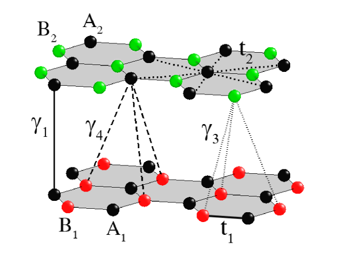
Figure 1: Crystalline structure of bilayer graphene. Atoms $A_{1}$ and $B_{1}$ in the lower monolayer are shown by red and black circles; black and green circles in the upper layer correspond to atoms $A_{2}$ and $B_{2}$. Intraplane electron hoppings are labeled by $t_{1}$ and $t_{2}$; $\gamma_{1},\,\gamma_{3}$ and $\gamma_{4}$ show the interlayer hoppings.

In this paper, in the Born weak-coupling approximation, we consider the Kohn-Luttinger superconducting pairing in an idealized graphene bilayer. We calculate the phase diagram, which reflects the competition between the superconducting phases with different types of the symmetry of the order parameter, taking into account the second-order contributions in the Coulomb interaction to the effective interaction of electrons in the Cooper channel. We analyze modification of the phase diagram with allowance for the Coulomb repulsion between electrons of the same, of the nearest, and of the next-to-nearest carbon atoms in a single layer, as well as the interlayer Coulomb interactions. We demonstrate the importance of taking into account the Coulomb repulsion of electrons on different crystal lattice sites and in different layers of bilayer graphene. The account of Coulomb repulsion changes the phase diagram of the superconducting state and, under certain conditions, increases the critical temperature.

2 Theoretical model

We consider an idealized graphene bilayer, assuming that two layers are arranged in accordance with the $AB$ type, i.e., one layer is rotated on 60^o relative to the other one McCann06 ; McCann13 . Let us choose the arrangement of the sublattices in the layers in such a way that the sites from different layers located one above another belong to the sublattices $A_{1}$ and $A_{2}$ respectively, while the other sites belong to the sublattices $B_{1}$ and $B_{2}$ (Fig. 1). In the Shubin-Vonsovsky (extended Hubbard) model Shubin34 , the Hamiltonian for the graphene bilayer which takes into account electron hoppings between the nearest and next-to-nearest atoms, as well as the Coulomb repulsion between electrons of the same and of the adjacent atoms and the interlayer Coulomb interaction of electrons, in the Wannier representation has the form:

$$\hat{H} = \hat{H}_{0}+\hat{H}_{int},$$ (1)

$$\hat{H}_{0} = (\varepsilon-\mu)\Biggl{(}\sum_{if\sigma}\hat{n}^{A}_{if\sigma}+\sum_{ig\sigma}\hat{n}^{B}_{ig\sigma}\Biggr{)}$$ (2)

$$- t_{1}\sum_{f\delta\sigma}(a^{{\dagger}}_{1f\sigma}b_{1,f+\delta,\sigma}+a^{{\dagger}}_{2f\sigma}b_{2,f-\delta,\sigma}+\textrm{h.c.})$$

$$- t_{2}\sum_{i\sigma}\Biggl{(}\sum_{\langle\langle fm\rangle\rangle}a^{{\dagger}}_{if\sigma}a_{im\sigma}+\sum_{\langle\langle gn\rangle\rangle}b^{{\dagger}}_{ig\sigma}b_{in\sigma}+\textrm{h.c.}\Biggr{)}$$

$$- \gamma_{1}\sum_{f\sigma}(a^{{\dagger}}_{1f\sigma}a_{2f\sigma}+\textrm{h.c.})$$

$$- \gamma_{3}\sum_{g\delta\sigma}(b^{{\dagger}}_{1g\sigma}b_{2,g+\delta,\sigma}+\textrm{h.c.})$$

$$- \gamma_{4}\sum_{f\delta\sigma}(a^{{\dagger}}_{1f\sigma}b_{2,f-\delta,\sigma}+a^{{\dagger}}_{2f\sigma}b_{1,f+\delta,\sigma}+\textrm{h.c.}),$$

$$\hat{H}_{int} = U\biggl{(}\sum_{if}\hat{n}^{A}_{if\uparrow}\hat{n}^{A}_{if\downarrow}+\sum_{ig}\hat{n}^{B}_{ig\uparrow}\hat{n}^{B}_{ig\downarrow}\biggr{)}+$$ (3)

$$+ V_{1}\sum_{f\delta\sigma\sigma^{\prime}}\Bigl{(}\hat{n}^{A}_{1f\sigma}\hat{n}^{B}_{1,f+\delta,\sigma^{\prime}}+\hat{n}^{A}_{2f\sigma}\hat{n}^{B}_{2,f-\delta,\sigma^{\prime}}\Bigr{)}+$$

$$+ \frac{V_{2}}{2}\sum_{i\sigma\sigma^{\prime}}\Biggl{(}\sum_{\langle\langle fm\rangle\rangle}\hat{n}^{A}_{if\sigma}\hat{n}^{A}_{im\sigma^{\prime}}+\sum_{\langle\langle gn\rangle\rangle}\hat{n}^{B}_{ig\sigma}\hat{n}^{B}_{in\sigma^{\prime}}\Biggr{)}+$$

$$+ G_{1}\sum_{f\sigma\sigma^{\prime}}\hat{n}^{A}_{1f\sigma}\hat{n}^{A}_{2f\sigma^{\prime}}+G_{3}\sum_{g\delta\sigma\sigma^{\prime}}\hat{n}^{B}_{1g\sigma}\hat{n}^{B}_{2,g+\delta,\sigma^{\prime}}+$$

$$+ G_{4}\sum_{f\delta\sigma\sigma^{\prime}}\Bigl{(}\hat{n}^{A}_{1f\sigma}\hat{n}^{B}_{2,f-\delta,\sigma^{\prime}}+\hat{n}^{A}_{2f\sigma}\hat{n}^{B}_{1,f+\delta,\sigma^{\prime}}\Bigr{)}.$$

In (1)–(3), the operators $a^{{\dagger}}_{1f\sigma}(a_{1f\sigma})$ create (annihilate) an electron with the spin projection $\sigma=\pm 1/2$ at site $f$ of the sublattice $A_{1}$; $\hat{n}^{A}_{1f\sigma}=a^{{\dagger}}_{1f\sigma}a_{1f\sigma}$ denotes the operators of the numbers of fermions at the $f$ site of the sublattice $A_{1}$ (analogous notations are used for the sublattices $A_{2}$, $B_{1}$, and $B_{2}$). Vector $\delta(-\delta)$ connects the nearest atoms of the hexagonal lattice of the lower (upper) layer. Index $i=1,2$ in Hamiltonian (1) denotes the number of layer. We assume that the one-site energies are identical ($\varepsilon_{Ai}=\varepsilon_{Bi}=\varepsilon$) and the position of the chemical potential $\mu$ and number of carriers $n$ in graphene bilayer can be controlled by a gate electric field. In the Hamiltonian, $t_{1}$ is the hopping integral between the neighboring atoms (hoppings between different sublattices), $t_{2}$ is the hopping integral between the next-to-nearest neighboring atoms (hoppings in the same sublattice), $U$ is the parameter of Coulomb repulsion between electrons of the same atom with the opposite spin projections (Hubbard repulsion), and $V_{1}$ and $V_{2}$ are the Coulomb interactions between electrons of the nearest and the next-to-nearest carbon atoms in a single layer. The symbol $\langle\langle~{}\rangle\rangle$ indicates that summation is made only over next-to-nearest neighbors; the symbols $\gamma_{1},\,\gamma_{3},\,\gamma_{4}$ denote the parameters of the interlayer electron hoppings (Fig. 1), and $G_{1}$, $G_{3}$ and $G_{4}$ are the interlayer Coulomb interactions between electrons.

We diagonalize the Hamiltonian $\hat{H}_{0}$ using the Bogolyubov transformation

$$\alpha_{i\vec{k}\sigma} = w_{i1}(\vec{k}){a_{1\vec{k}\sigma}}+w_{i2}(\vec{k}){a_{2\vec{k}\sigma}}$$

$$+ w_{i3}(\vec{k}){b_{1\vec{k}\sigma}}+w_{i4}(\vec{k}){b_{2\vec{k}\sigma}},\quad i=1,2,3,4.$$

As a result, $\hat{H}_{0}$ acquires the form

$$\hat{H}_{0}=\sum\limits_{i=1}^{4}\sum\limits_{\vec{k}\sigma}E_{i\vec{k}}{\alpha_{i\vec{k}\sigma}^{{\dagger}}\alpha_{i\vec{k}\sigma}}.$$ (5)

Since the results of ab initio calculations for graphite Dresselhaus02 ; Brandt88 showed a very small value of the interlayer hopping parameter $\gamma_{4}$, hereinafter we assume that $\gamma_{4}=0$. Then, the four-band energy spectrum of the graphene bilayer is described by the expressions

$$E_{i\vec{k}}=\varepsilon\pm\sqrt{A_{\vec{k}}\pm\sqrt{B_{\vec{k}}}}-t_{2}f_{\vec{k}},$$ (6)

$$A_{\vec{k}}=\frac{1}{4}\Bigl{(}2a^{2}+4|b_{\vec{k}}|^{2}+2|d_{\vec{k}}|^{2}\Bigr{)},$$

$$B_{\vec{k}}=\frac{1}{4}\Bigl{(}|d_{\vec{k}}|^{2}(|d_{\vec{k}}|^{2}-2a^{2}+4|b_{\vec{k}}|^{2})+a^{4}+4a^{2}|b_{\vec{k}}|^{2}$$

$$\qquad+4ab^{2}_{\vec{k}}d_{\vec{k}}+4ab_{\vec{k}}^{*2}d^{*}_{\vec{k}}\Bigr{)},$$

$$a=\gamma_{1},\quad b_{\vec{k}}=t_{1}u_{\vec{k}},\quad d_{\vec{k}}=\gamma_{3}u_{\vec{k}},$$

where the following notation has been introduced:

$$f_{\vec{k}}=2\cos(\sqrt{3}k_{y})+4\cos\biggl{(}\frac{\sqrt{3}}{2}k_{y}\biggr{)}\cos\biggl{(}\frac{3}{2}k_{x}\biggr{)},$$ (7)

$$u_{\vec{k}}=\displaystyle\sum_{\delta}e^{i\vec{k}\delta}=e^{-ik_{x}}+2e^{\frac{i}{2}k_{x}}\cos\biggl{(}\frac{\sqrt{3}}{2}k_{y}\biggr{)},$$ (8)

$$|u_{\vec{k}}|=\sqrt{3+f_{\vec{k}}}.$$ (9)

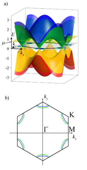
Figure 2: (a) Energy bands of graphene bilayer in the vicinity of the Dirac points and (b) formation of the Fermi contour at $t_{2}=0,\,\gamma_{1}=0.12,\,\gamma_{3}=0.1$, and $\mu=0.7$ (all the parameters are given in units of $|t_{1}|$).

In this paper, the conditions for the implementation of the Kohn-Luttinger superconductivity are analyzed by considering the situation when upon doping of the graphene bilayer the chemical potential falls into the two upper energy bands $E_{1\vec{k}}$ and $E_{2\vec{k}}$ (Fig. 2a). Then, if $\gamma_{1}\neq 0$ and the inequality $\mu>\gamma_{1}$ is valid, the Fermi contour will consist of two lines (Fig. 2b) in the vicinity of each Dirac point for the electron densities $1<n<n_{VH}$, where $n$ is the electron density calculated per atoms of one layer.

The coefficients of the Bogolyubov transformation can be found from the system of homogeneous equations

$$\left(\begin{array}[]{cccc}x_{i}&a&b^{*}_{\vec{k}}&0\\ a&x_{i}&0&b_{\vec{k}}\\ b_{\vec{k}}&0&x_{i}&d^{*}_{\vec{k}}\\ 0&b^{*}_{\vec{k}}&d_{\vec{k}}&x_{i}\\ \end{array}\right)\left(\begin{array}[]{c}w_{i1}\\ w_{i2}\\ w_{i3}\\ w_{i4}\\ \end{array}\right)=0,$$ (18)

where $x_{i}=E_{i\vec{k}}-\varepsilon+t_{2}f_{\vec{k}}$.

In the Bogolyubov representation, the Hamiltonian $\hat{H}_{int}$ (3) in terms of the operators $\alpha_{1\vec{k}\sigma},\,\alpha_{2\vec{k}\sigma},\,\alpha_{3\vec{k}\sigma}$ and $\alpha_{4\vec{k}\sigma}$ reads as follows:

$$\hat{H}_{int} = \frac{1}{N}\sum\limits_{ijlm\sigma\atop\vec{k}\vec{p}\vec{q}\vec{s}}\Gamma_{ij;lm}^{||}(\vec{k},\vec{p}|\vec{q},\vec{s})\alpha_{i\vec{k}\sigma}^{\dagger}\alpha_{j\vec{p}\sigma}^{\dagger}\alpha_{l\vec{q}\sigma}\alpha_{m\vec{s}\sigma}$$

$$\times \delta(\vec{k}+\vec{p}-\vec{q}-\vec{s})$$

$$+ \frac{1}{N}\sum\limits_{ijlm\atop\vec{k}\vec{p}\vec{q}\vec{s}}\Gamma_{ij;lm}^{\bot}(\vec{k},\vec{p}|\vec{q},\vec{s})\alpha_{i\vec{k}\uparrow}^{\dagger}\alpha_{j\vec{p}\downarrow}^{\dagger}\alpha_{l\vec{q}\downarrow}\alpha_{m\vec{s}\uparrow}$$

$$\times \delta(\vec{k}+\vec{p}-\vec{q}-\vec{s}),$$

where $\delta(x)$ is the Dirac delta-function and $\Gamma_{ij;lm}^{||}(\vec{k},\vec{p}|\vec{q},\vec{s})$ and $\Gamma_{ij;lm}^{\bot}(\vec{k},\vec{p}|\vec{q},\vec{s})$ are the initial amplitudes. The quantity

$$\Gamma_{ij;lm}^{||} (\vec{k},\vec{p}|\vec{q},\vec{s})$$ (20)

$$=\frac{1}{2}\Bigl{(}V_{ij;lm}(\vec{k},\vec{p}|\vec{q},\vec{s})+V_{ji;ml}(\vec{p},\vec{k}|\vec{s},\vec{q})$$

$$+G^{(1)}_{ij;lm}(\vec{k},\vec{p}|\vec{q},\vec{s})+G^{(1)}_{ji;ml}(\vec{p},\vec{k}|\vec{s},\vec{q})$$

$$+G^{(3)}_{ij;lm}(\vec{k},\vec{p}|\vec{q},\vec{s})+G^{(3)}_{ji;ml}(\vec{p},\vec{k}|\vec{s},\vec{q})$$

$$+G^{(4)}_{ij;lm}(\vec{k},\vec{p}|\vec{q},\vec{s})+G^{(4)}_{ji;ml}(\vec{p},\vec{k}|\vec{s},\vec{q})\Bigr{)},$$

$$V_{ij;lm} (\vec{k},\vec{p}|\vec{q},\vec{s})=V_{1}\Bigl{(}u_{\vec{q}-\vec{p}}w_{i1}(\vec{k})w_{j3}(\vec{p})w^{*}_{l3}(\vec{q})w^{*}_{m1}(\vec{s})$$ (21)

$$+u_{\vec{q}-\vec{p}}^{*}w_{i2}(\vec{k})w_{j4}(\vec{p})w^{*}_{l4}(\vec{q})w^{*}_{m2}(\vec{s})\Bigr{)}$$

$$+\frac{V_{2}}{2}\sum_{r=1}^{4}f_{\vec{q}-\vec{p}}w_{ir}(\vec{k})w_{jr}(\vec{p})w^{*}_{lr}(\vec{q})w^{*}_{mr}(\vec{s}),$$

$$G^{(1)}_{ij;lm} (\vec{k},\vec{p}|\vec{q},\vec{s})=G_{1}w_{i1}(\vec{k})w_{j2}(\vec{p})w^{*}_{l2}(\vec{q})w^{*}_{m1}(\vec{s}),$$ (22)

$$G^{(3)}_{ij;lm} (\vec{k},\vec{p}|\vec{q},\vec{s})$$ (23)

$$=G_{3}u_{\vec{q}-\vec{p}}w_{i3}(\vec{k})w_{j4}(\vec{p})w^{*}_{l4}(\vec{q})w^{*}_{m3}(\vec{s}),$$

$$G^{(4)}_{ij;lm} (\vec{k},\vec{p}|\vec{q},\vec{s})=G_{4}\Bigl{(}u_{\vec{q}-\vec{p}}^{*}w_{i1}(\vec{k})w_{j4}(\vec{p})w^{*}_{l4}(\vec{q})w^{*}_{m1}(\vec{s})$$ (24)

$$+u_{\vec{q}-\vec{p}}w_{i2}(\vec{k})w_{j3}(\vec{p})w^{*}_{l3}(\vec{q})w^{*}_{m2}(\vec{s})\Bigr{)}$$

corresponds to the intensity of the interaction of fermions with parallel spin projections, while the quantity

$$\Gamma_{ij;lm}^{\bot} (\vec{k},\vec{p}|\vec{q},\vec{s})=U_{ij;lm}(\vec{k},\vec{p}|\vec{q},\vec{s})$$ (25)

$$+V_{ij;lm}(\vec{k},\vec{p}|\vec{q},\vec{s})+V_{ji;ml}(\vec{p},\vec{k}|\vec{s},\vec{q})$$

$$+G^{(1)}_{ij;lm}(\vec{k},\vec{p}|\vec{q},\vec{s})+G^{(1)}_{ji;ml}(\vec{p},\vec{k}|\vec{s},\vec{q})$$

$$+G^{(3)}_{ij;lm}(\vec{k},\vec{p}|\vec{q},\vec{s})+G^{(3)}_{ji;ml}(\vec{p},\vec{k}|\vec{s},\vec{q})$$

$$+G^{(4)}_{ij;lm}(\vec{k},\vec{p}|\vec{q},\vec{s})+G^{(4)}_{ji;ml}(\vec{p},\vec{k}|\vec{s},\vec{q}),$$

$$U_{ij;lm} (\vec{k},\vec{p}|\vec{q},\vec{s})$$ (26)

$$=U\sum_{r=1}^{4}w_{ir}(\vec{k})w_{jr}(\vec{p})w^{*}_{lr}(\vec{q})w^{*}_{mr}(\vec{s})$$

describes the interaction of fermions with antiparallel spin projections. Indices ${i,j,l,m}$ correspond to the number of the energy band and acquire the values 1, 2, 3, or 4.

3 Effective interaction and equation for the superconducting order parameter

In this paper, we use the Born weak-coupling approximation, in which the hierarchy of model parameters has the form

$$W>U>V_{1}>V_{2}>G_{1}>G_{3},\,G_{4},$$ (27)

where $W$ is the bandwidth in graphene bilayer (6). In the calculation of the scattering amplitude in the Cooper channel, the condition (27) allows us to limit the consideration to only the second-order diagrams in the effective interaction of two electrons with opposite values of the momentum and spin and use the quantity $\widetilde{\Gamma}(\vec{p},\vec{k})$ for it. Figure 3 depicts the sum of diagrams which determines $\widetilde{\Gamma}(\vec{p},\vec{k})$. Here, solid lines correspond to Green’s functions for the electrons with opposite spin projections $+\frac{1}{2}$ (light arrows) and $-\frac{1}{2}$ (black arrows). The first diagram describes the initial interaction of two electrons in the Cooper channel. Here, the wavy lines correspond to the initial interaction. The next four diagrams in Fig. 3 correspond to the second-order scattering processes $\delta\widetilde{\Gamma}(\vec{p},\vec{k})$ and describe the polarization effects of the filled Fermi sphere. In the diagrams, the presence of solid lines without arrows means the summation over the spin projections values.

The possibility of the Cooper pairing is determined by the features of the energy structure and the effective interaction of electrons near the Fermi level Gor'kov61 . If we assume that the chemical potential in doped graphene bilayer is located in the two upper bands $E_{1\vec{k}}$ and $E_{2\vec{k}}$ (Fig. 2a), we can consider the situation in which the initial and final momenta of electrons in the Cooper channel also belong to the two upper bands and analyze the conditions for the Kohn-Luttinger superconducting pairing. At that, indices $i$ and $j$ in the diagrams (Fig. 3) will acquire the values of 1 or 2.

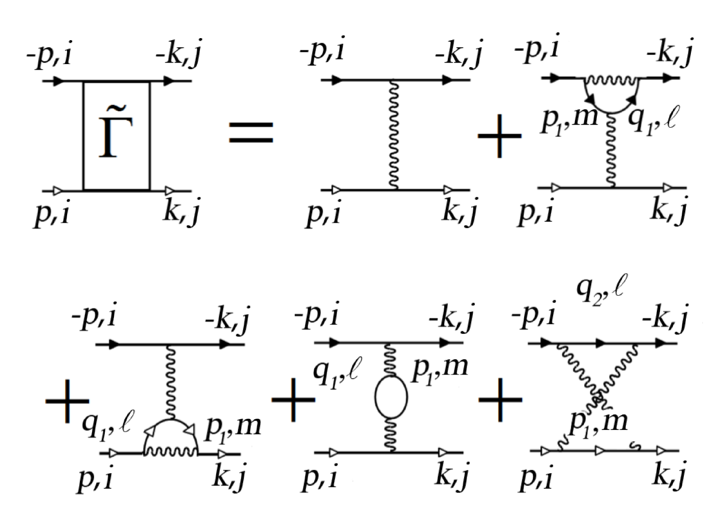
Figure 3: The sum of diagrams for the effective interaction of electrons in the Cooper channel for graphene bilayer. Solid lines correspond to Green’s functions for electrons with spin projections $+{\textstyle{1\over 2}}$ and $-{\textstyle{1\over 2}}$ and energies corresponding to the energy bands $E_{i}$, $E_{j}$, $E_{l}$, and $E_{m}$. Subscripts $i$ and $j$ acquire the values of 1 or 2, whereas $l$ and $m$ acquire the values of 1, 2, 3, or 4. Momenta $\vec{q}_{1}$ and $\vec{q}_{2}$ are defined by (32).

Introducing the analytical expressions for the diagrams, we get the effective interaction in the form

$$\widetilde{\Gamma}(\vec{p},\vec{k})=\widetilde{\Gamma}_{0}(\vec{p},\vec{k})+\delta\widetilde{\Gamma}(\vec{p},\vec{k}),$$ (28)

$$\widetilde{\Gamma}_{0}(\vec{p},\vec{k})=\Gamma^{\bot}_{ii;jj}(\vec{p},-\vec{p}|-\vec{k},\vec{k}),$$ (29)

$$\delta\tilde{\Gamma}(\vec{p},\vec{k})=\frac{1}{N}\sum\limits_{l,m,\vec{p}_{1}}\Gamma^{\bot}_{il;jm}(\vec{p},\vec{q}_{2}|-\vec{k},\vec{p}_{1})$$ (30)

$$\times\Gamma^{\bot}_{mi;lj}(\vec{p}_{1},-\vec{p}|\vec{q}_{2},\vec{k})\chi_{l,m}(\vec{q}_{2},\vec{p}_{1})$$

$$+\frac{2}{N}\sum\limits_{l,m,\vec{p}_{1}}\Bigl{\{}\Gamma^{\bot}_{im;lj}(\vec{p},\vec{p}_{1}|\vec{q}_{1},\vec{k})$$

$$\times\left[\Gamma^{||}_{li;mj}(\vec{q}_{1},-\vec{p}|\vec{p}_{1},-\vec{k})-\Gamma^{||}_{li;jm}(\vec{q}_{1},-\vec{p}|-\vec{k},\vec{p}_{1})\right]\Bigr{.}$$

$$+\Bigl{.}\Gamma^{\bot}_{li;jm}(\vec{q}_{1},-\vec{p}|-\vec{k},\vec{p}_{1})$$

$$\times\left[\Gamma^{||}_{im;jl}(\vec{p},\vec{p}_{1}|\vec{k},\vec{q}_{1})-\Gamma^{||}_{im;lj}(\vec{p},\vec{p}_{1}|\vec{q}_{1},\vec{k})\right]\Bigr{\}}\chi_{l,m}(\vec{q}_{1},\vec{p}_{1}).$$

Here, we use the notations for the generalized susceptibilities

$$\chi_{l,m}(\vec{k},\vec{p})=\frac{f(E_{l\vec{k}})-f(E_{m\vec{p}})}{E_{m\vec{p}}-E_{l\vec{k}}},$$ (31)

where $f(x)=(\exp(\frac{x-\mu}{T})+1)^{-1}$ is the Fermi-Dirac function and the energies $E_{i\vec{k}}$ are defined by the expressions (6). Additionally, we have introduced the following notations for the combinations of the momenta

$$\vec{q}_{1}=\vec{p}_{1}+\vec{p}-\vec{k},\qquad\vec{q}_{2}=\vec{p}_{1}-\vec{p}-\vec{k}.$$ (32)

The renormalized expression for the effective interaction allows us to analyze the conditions for the occurrence of superconductivity in the system. It is known Gor'kov61 that the development of the Cooper instability can be established from the consideration of the homogeneous part of the Bethe-Salpeter equation. At that, the dependence of the scattering amplitude $\Gamma(\vec{p},\vec{k})$ on momentum $\vec{k}$ is factorized and we get the integral equation for the superconducting order parameter $\Delta(\vec{p})$. After the integration over the isoenergetic contours, the problem of the Cooper instability can be reduced to the eigenvalue problem Scalapino86 ; Baranov92 ; Hlubina99 ; Raghu10 ; Alexandrov11

$$\frac{3\sqrt{3}}{8\pi^{2}}\oint\limits_{\varepsilon_{\vec{q}}=\mu}\frac{d\hat{\vec{q}}}{v_{F}(\hat{\vec{q}})}\widetilde{\Gamma}(\hat{\vec{\vec{p}}},\hat{\vec{q}})\Delta(\hat{\vec{q}})=\lambda\Delta(\hat{\vec{p}}),$$ (33)

where the eigenvector is the superconducting order parameter $\Delta(\hat{\vec{q}})$ and the eigenvalues $\lambda$ satisfy the relation $\lambda^{-1}\simeq\ln(T_{c}/W)$. Here, the momenta $\hat{\vec{p}}$ and $\hat{\vec{q}}$ belong to the Fermi surface and $v_{F}(\hat{\vec{q}})$ is the Fermi velocity. Equation (33) is solved in accordance with the common scheme described in Kagan14 ; Kagan14a . The integration is fulfilled with the allowance for the fact that the Fermi contour near each Dirac point consists of two lines (Fig. 2b).

4 Results and discussion

Let us consider the phase diagram of the superconducting state of the graphene bilayer and the modifications of this diagram in the different regimes obtained by solving Eq. (33). When building the phase diagram, we divided the multisheet Fermi contour into 180 intervals and the Brillouin zone of the graphene bilayer, into $5\cdot 10^{4}$ cells. It was established that the chosen method of division is sufficient for the correct description of the dependence of the effective coupling constant $\lambda$ on the electron density $n$ Kagan14 . Based on the obtained dependences $\lambda(n)$ for different values of the intersite $V_{1}$ and interplane $G_{1},\,G_{3}$ and $G_{4}$ Coulomb interactions, we built the phase diagrams of the Shubin-Vonsovsky model for bilayer graphene, which reflect the competition between the superconducting phases with different types of symmetry of the order parameter.

So far, there has been no agreement regarding the values of parameters of the intra- and interplanar Coulomb interactions in the graphene bilayer. The ab initio calculations for graphite Wehling11 showed that the value of Hubbard repulsion is $U=8.0\,\textrm{eV}$, which is consistent with the estimation made in Levin74 and contradicts the intuitively expected small value of $U$ and weak-coupling limit $U<W$ (it is known Reich02 that $t_{1}\approx 2.8\,\textrm{eV}$). The authors of Wehling11 calculated the parameters of Coulomb repulsion between electrons of the nearest and the next-to-nearest carbon atoms: $V_{1}=3.9\,\textrm{eV}$ and $V_{2}=2.4\,\textrm{eV}$, respectively. At the same time, the other authors (see, for example, Perfetto07 ) consider these parameters to be much smaller. The authors of Milovanovic12 mentioned that the estimation of the parameters of Coulomb interaction, including the Hubbard repulsion, in the graphene bilayer strongly depends on the calculation scheme which is used. In our calculation, we apply the parameter hierarchy (27), which allows us to use the Born weak-coupling approximation. For interlayer hopping parameters $\gamma_{1}$ and $\gamma_{3}$, we use the values similar to those determined in Dresselhaus02 ; Brandt88 for graphite.

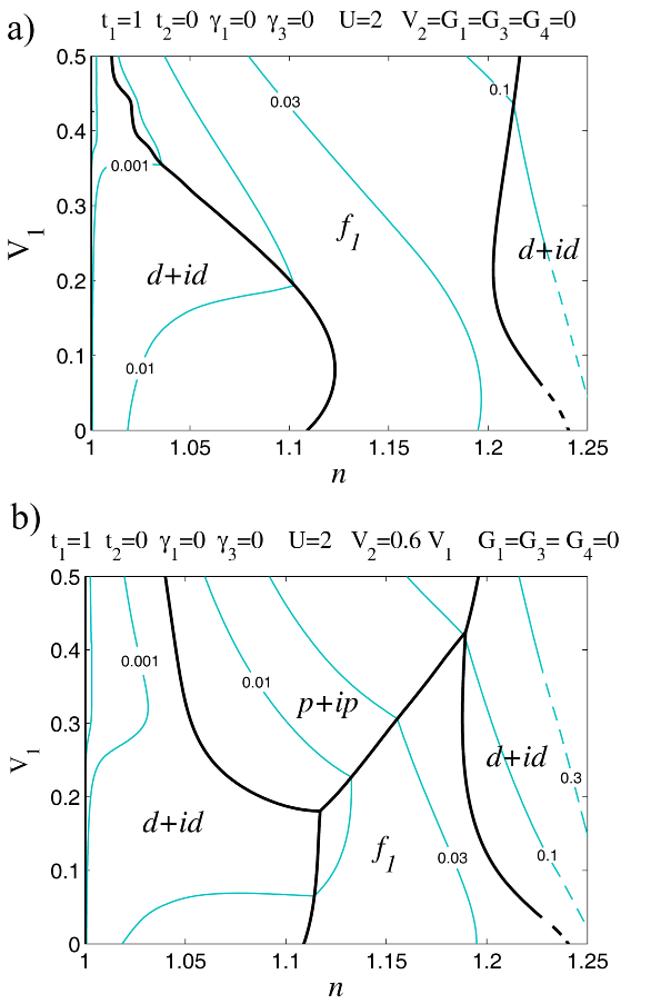
Figure 4: Phase diagram of the superconducting state of the graphene bilayer shown as a function of the variables ”$n-V_{1}$” at $t_{2}=0,\,\gamma_{1}=\gamma_{3}=0,\,U=2,\,G_{1}=G_{3}=G_{4}=0$ for (a) $V_{2}=0$ and (b) $V_{2}=0.6V_{1}$ (all the parameters are in units of $|t_{1}|$). For all the points on the same thin blue line, the value of $|\lambda|$ is constant and marked with the corresponding number.

First, let us consider the limiting case when the bilayer energy spectrum is described by the only one hopping parameter ($t_{1}\neq 0,\,t_{2}=\gamma_{1}=\gamma_{3}=0$). The Hubbard repulsion is also taken into account $U=2$ (hereinafter, all the parameters are given in units of $|t_{1}|$). The Coulomb repulsion between electrons ($V_{1}\neq 0$) of the neighboring carbon atoms in the same layer is taken into account as well. At the same time, the interlayer Coulomb interactions are not taken into account ($G_{1}=G_{3}=G_{4}=0$). Thus, in the chosen regime, the graphene bilayer consists of two isolated single layers. The phase diagram of the superconducting state shown as a function of the variables ”$n-V_{1}$” for this case is presented in Fig. 4a. It can be seen that the phase diagram comprises three regions. At low electron densities $n$, the ground state of the system corresponds to the superconductivity with the $d+id-$wave symmetry of the order parameter, which is described by the 2D representation $E_{2}$, the contribution to which is determined by the harmonics

$$g_{m}^{(d+id)}(\phi)=\frac{1}{\sqrt{\pi}}\,(A\,\textrm{sin}\,(2m+2)\phi+B\,\textrm{cos}\,(2m+2)\phi),$$

where subscripts $m$ run over the values for which the coefficients $(2m+2)$ are not multiples of 3. At the intermediate electron densities, the superconducting $f-$wave pairing is implemented, the contribution to which is determined by the harmonics $g_{m}^{(f_{1})}(\phi)=\displaystyle\frac{1}{\sqrt{\pi}}\,\textrm{sin}\,(6m+3)\phi$ (here $m\in[\,0,\infty)$), while the contribution of the harmonics $g_{m}^{(f_{2})}(\phi)=\displaystyle\frac{1}{\sqrt{\pi}}\,\textrm{cos}\,(6m+3)\phi$ is absent. At the large values of $n$, the domain of the superconducting $d+id-$wave pairing occurs Nandkishore12 . With the increase of the parameter $V_{1}$ of the intersite Coulomb interaction, in the region of small values of $n$, the $d+id-$wave pairing is suppressed and the pairing with the $f-$wave symmetry of the order parameter is implemented. Thin blue lines in Fig. 4 are the lines of the equal values of the effective coupling constant $|\lambda|$. It can be seen that in this case in the proximity of the Van Hove filling $n_{VH}$ (solid curve in Fig. 5) the effective coupling constant attains the values $|\lambda|=0.1$.

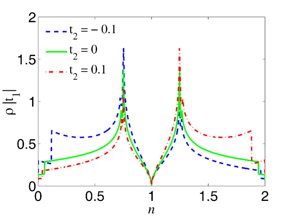
Figure 5: Modification of the dependence of the density of electron states of the graphene bilayer from electron density calculated for atoms in the same layer with respect to electron hoppings to the next-to-nearest neighboring atoms.

It should be noted that to avoid the summation of the parquet diagrams Dzyaloshinskii88a ; Dzyaloshinskii88b ; Zheleznyak97 , we do not analyze here the electron density regions that are very close to the Van Hove singularity in the density of electron states of bilayer graphene (Fig. 5). For this reason, the boundaries between different domains of the implementation of the Kohn-Luttinger superconducting pairing, as well as the lines of the equal value of $|\lambda|$ that are very close to the Van Hove singularity are indicated in the phase diagram by the dashed lines.

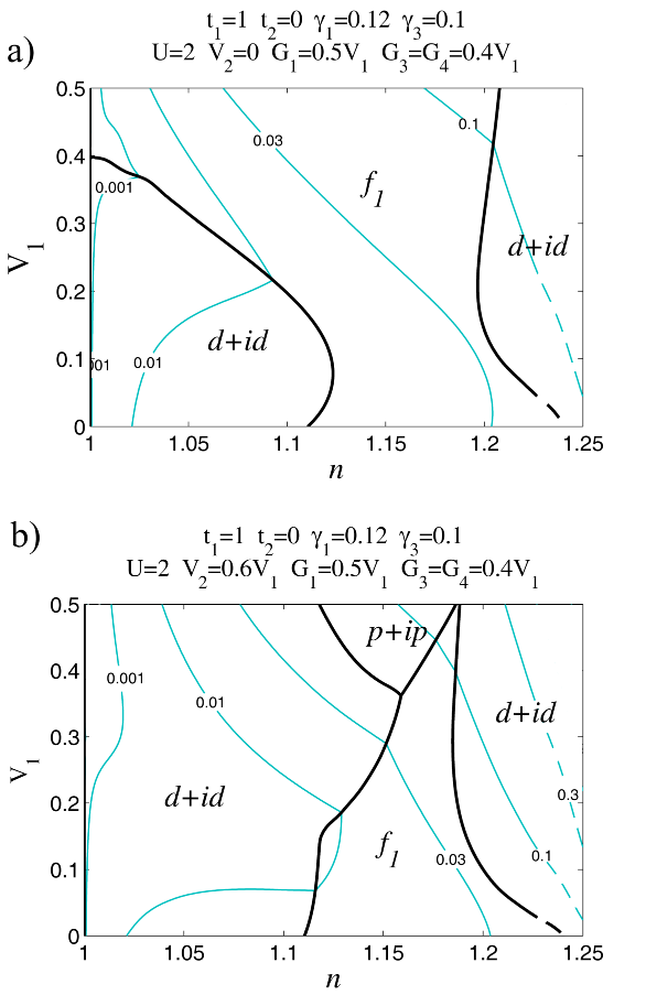
Figure 6: Phase diagram of the superconducting state of the graphene bilayer shown as a function of the variables ”$n-V_{1}$” for $t_{2}=0,\,\gamma_{1}=0.12,\,\gamma_{3}=0.1,\,U=2,\,G_{1}=0.5V_{1},\,G_{3}=G_{4}=0.4V_{1}$, at (a) $V_{2}=0$ and (b) $V_{2}=0.6V_{1}$ (all the parameters are given in units of $|t_{1}|$). Thin blue curves are the lines of the constant values of $|\lambda|$.

Thus, in the numerical calculation for the graphene bilayer for the chosen parameters, we made the limiting transition to the results obtained by us previously for the graphene monolayer Kagan14 ; Kagan14a .

Let us consider the modification of the phase diagram for the isolated graphene single layers with regard to the long-range intraplane Coulomb interactions between electrons $V_{2}$. It can be seen in Fig. 4b for the fixed ratio between the parameters of the long-range Coulomb interactions $V_{2}=0.6V_{1}$ that when $V_{2}$ is taken into account, the phase diagram changes qualitatively. This change involves the suppression of a large domain of the superconducting state with the $f-$wave symmetry at the intermediate electron densities and the implementation of the superconducting pairing with the $p+ip-$wave symmetry of the order parameter. In addition, when $V_{2}$ is taken into account, the effective coupling constant increases to the value $|\lambda|=0.3$.

Now, let us consider the modification of the phase diagram of the superconducting state with respect to the interplanar interactions. When the interlayer electron hoppings $\gamma_{1}=0.12$ and $\gamma_{3}=0.1$ are taken into account while the other parameters being the same as in Fig. 4, the phase diagram of the graphene bilayer remains nearly unchanged.

Inclusion of the Coulomb interaction $G_{1}$ in the consideration weakly shifts the boundaries of the $f_{1}-$wave and $d+id-$wave pairing in the phase diagram in Fig. 4 and does not affect the absolute values of $\lambda$. Figure 6 shows the effect of taking into account the interlayer Coulomb interactions $G_{3}$ and $G_{4}$. Figure 6a shows the phase diagram of the Shubin-Vonsovsky model for the graphene bilayer for the set of parameters $t_{2}=0,\,\gamma_{1}=0.12,\,\gamma_{3}=0.1,\,U=2$ and $V_{2}=0$ for the chosen ratios between the interlayer and intersite Coulomb interactions $G_{1}=0.5V_{1},\,G_{3}=G_{4}=0.4V_{1}$, according to the hierarchy of the parameters (27). The calculation shows that the separate increase of the parameters $G_{3}$ and $G_{4}$ suppresses the $d+id-$wave pairing and, at the same time, broadens the $f-$wave pairing region at small electron densities. The superconducting $d+id-$phase is suppressed the most effectively by enhancing the parameter $G_{4}$ of the interlayer Coulomb interaction. When the interactions $G_{3}$ and $G_{4}$ are simultaneously taken into account (Fig. 6a), then along with the intensive suppression of the superconducting $d+id-$wave pairing at small electron densities and the implementation of the superconductivity with the $f-$wave symmetry of the order parameter, the growth of the absolute values of effective coupling constant $\lambda$ is also observed.

Figure 6b depicts the phase diagram of the graphene bilayer calculated for the same parameters as in Fig. 6a but with respect to the long-range intraplane Coulomb repulsion between electrons $V_{2}$. Comparison of Figs. 6b and  4b shows that the account for $G_{3}\neq 0$ and $G_{4}\neq 0$ leads to the strong competition between the $d+id-$wave and $p+ip-$wave pairings with the significant suppression of the $p+ip-$wave pairing in the region of the intermediate electron densities. In this case, in the remained region of the $p+ip-$wave pairing, $|\lambda_{p+ip}|$ slightly exceeds $|\lambda_{f}|$.

The account for electron hoppings to the next-to-nearest carbon atoms $t_{2}$ does not qualitatively affects the competition between the superconducting phases (Fig. 6). Figure 7 depicts the phase diagram of the graphene bilayer obtained for the parameters $t_{2}=0.1,\,\gamma_{1}=0.12,\,\gamma_{3}=0.1,\,U=2,\,G_{1}=0.5V_{1}$ and $G_{3}=G_{4}=0.4V_{1}$. Such a behavior of the system is explained by the fact that switching on of the hoppings $t_{2}>0$ or $t_{2}<0$ for the graphene bilayer, similarly to the case of the monolayer investigated by us in Kagan14 ; Kagan14a , does not significantly modify the density of electron states in the carrier concentration regions between the Dirac point and both points $n_{VH}$ (Fig. 5). However, it can be seen in Fig. 7 that the account for the hoppings $t_{2}$ leads to an increase of the effective interaction in the absolute values and, consequently, to the higher superconducting transition temperatures in an idealized graphene bilayer.

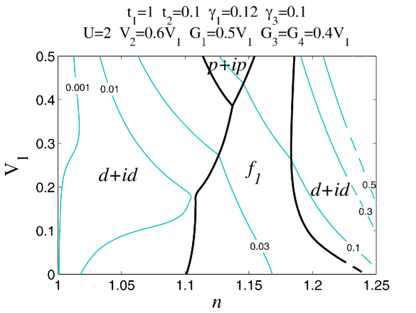
Figure 7: Phase diagram of the superconducting state of the graphene bilayer shown as a function of the variables ”$n-V_{1}$” at $t_{2}=0.1,\,\gamma_{1}=0.12,\,\gamma_{3}=0.1,\,U=2,\,G_{1}=0.5V_{1},\,G_{3}=G_{4}=0.4V_{1}$ (all the parameters are in units of $|t_{1}|$). Thin blue curves are the lines of the constant values of $|\lambda|$.

It should be noted that the Kohn–Luttinger superconductivity in the graphene single layer and bilayer never develops near the Dirac points. The calculations show that in the vicinity of these points, where the linear approximation for the energy spectrum of the graphene single layer and the parabolic approximation for the spectrum of the graphene bilayer work pretty well, the density of states is very low and the effective coupling constant $|\lambda|<10^{-2}$. The higher values of $|\lambda|$, which are indicative of the development of the Cooper instability, arise at the electron densities $n>1.15$. However, at such densities, the energy spectrum of the bilayer along the direction $KM$ of the Brillouin zone (Fig. 2b) already significantly differs from the Dirac approximation.

5 Conclusions

In the work, we have analyzed the conditions for the Kohn-Luttinger superconductivity in a semimetal with the Dirac spectrum using as an example an idealized graphene bilayer, disregarding the van der Waals potential of the substrate and both magnetic and non-magnetic impurities. The electronic structure of graphene bilayer is described in the Shubin-Vonsovsky model taking into account not only the Coulomb repulsion of electrons of the same carbon atom, but also the intersite and interlayer Coulomb interactions. It was shown that in such a system, the Kohn-Luttinger polarization contributions lead to the effective attraction between electrons in the Cooper channel. The constructed superconducting phase diagram of the system determines the Cooper pairing domains with the different types of the symmetry of the order parameter, depending on the intersite Coulomb interactions and the electron densities. The analysis of the phase diagram showed that the inclusion of the Kohn-Luttinger renormalizations up to the second order of perturbation theory inclusively and the allowance for the long-range Coulomb interactions $V_{1}$ and $V_{2}$ determine, to a considerable extent, the competition between the superconducting phases with the $f-$wave, $p+ip-$wave, and $d+id$-wave types of the symmetry of the order parameter. They also lead to a significant increase in the absolute values of the effective interaction. It was shown that the allowance for the interlayer Coulomb interactions $G_{3}$ and $G_{4}$, as well as for the distant electron hoppings $t_{2}$, leads to an additional increase in the effective interaction and, hence, to the higher superconducting transition temperatures in an idealized graphene bilayer.

Our calculation showed that the Kohn-Luttinger mechanism can lead to the superconducting transition temperatures $T_{c}\sim 20\div 40~{}K$ in an idealized graphene bilayer. Contrary to these rather optimistic estimations, in real graphene, as it was mentioned in Introduction, superconductivity has not been found yet. This material is only close to superconductivity.

For a few reasons, the results of the theoretical calculations reported here can differ from the experimental situation. First, we did not take into account the effect of the van der Waals potential of the substrate Gomez09 ; Bostrom12 ; Klimchitskaya13 . It seems that the effect of this potential should be weakened with the increase of number of layers. However, even in the multilayer systems the van der Waals forces can degrade the conditions for the development of the Cooper instability.

Second, as we mentioned in Section 4, there has been no agreement regarding the values of the parameters of the intraplane and interplanar Coulomb interactions in the graphene bilayer in the literature. In this work, we used the values of the intraplane Coulomb interactions that are close to those obtained from the ab initio calculation in Wehling11 for graphite. The values of the interplanar Coulomb interactions were chosen to satisfy the hierarchy of the parameters of the Born weak-coupling approximation.

Third, in our calculations, we considered a pure graphene bilayer with the ideal structure, whereas the real material contains numerous impurities and structural defects. It is well known that, in contrast to the traditional $s-$wave pairing, for the anomalous pairing with the $f$-wave, $p+ip$-wave, and $d+id$-wave symmetries of the order parameter, nonmagnetic impurities and structural defects can destroy the superconducting order Black14b .

In addition, we should mention one more possible reason for the discrepancy between the theoretical calculations on superconductivity in graphene and the experimentally observed situation. In recent paper Kats14 , the effect of quantum fluctuations ($T=0$) on the graphene layers was investigated. It was shown that these fluctuations initiate the logarithmic corrections to the moduli of elasticity and bending of the layers. In other words, according to Kats14 , the quantum fluctuations connected with the bending vibrations of the graphene layers can lead to the situation when the electrons do not move along the atomically smooth layers but along the strongly curved string-like trajectories, as in quantum chromodynamics. This situation requires further investigations, although in this case the superconductivity is not at all excluded and even can be enhanced by the exchange of bending vibration quanta between the pairing electrons.

We thank V.V. Val’kov for useful discussions. This work is supported by the Russian Foundation for Basic Research (projects nos. 14-02-00058 and 14-02-31237). One of the authors (M. Yu. K.) gratefully acknowledges support from the Basic Research Program of the National Research University Higher School of Economics. Another one (M. M. K.) thanks the scholarship SP-1361.2015.1 of the President of the Russian Federation and the Dynasty foundation.

References

- (1) H. B. Heersche, P. Jarillo-Herrero, J. B. Oostinga, L. M. K. Vandersypen, A. F. Morpurgo, Nature (London) 446, 56 (2007)
- (2) A. Shailos, W. Nativel, A. Kasumov, C. Collet, M. Ferrier, S. Gueron, R. Deblock, H. Bouchiat, Europhys. Lett. 79, 57008 (2007)
- (3) X. Du, I. Skachko, E. Y. Andrei, Phys. Rev. B 77, 184507 (2008)
- (4) C. Ojeda-Aristizabal, M. Ferrier, S. Guéron, H. Bouchiat, Phys. Rev. B 79, 165436 (2009)
- (5) A. Kanda, T. Sato, H. Goto, H. Tomori, S. Takana, Y. Ootuka, K. Tsukagoshi, Physica C 470, 1477 (2010)
- (6) Z. Han, A. Allain, H. Arjmandi-Tash, K. Tikhonov, M. Feigel’man, B. Sacépé, V. Bouchiat, Nature Phys. 10, 380 (2014)
- (7) N. B. Kopnin, E. B. Sonin, Phys. Rev. Lett. 100, 246808 (2008)
- (8) D. M. Basko, I. L. Aleiner, Phys. Rev. B 77, 041409(R) (2008)
- (9) Yu. E. Lozovik, A. A. Sokolik, Eur. Phys. J. B 73, 195 (2010)
- (10) M. Einenkel, K. B. Efetov, Phys. Rev. B 84, 214508 (2011)
- (11) L. Classen, M. M. Scherer, C. Honerkamp, Phys. Rev. B 90, 035122 (2014)
- (12) A. M. Black-Schaffer, S. Doniach, Phys. Rev. B 75, 134512 (2007)
- (13) C. Honerkamp, Phys. Rev. Lett. 100, 146404 (2008)
- (14) J. Vučičević, M. O. Goerbig, M. V. Milovanović, Phys. Rev. B 86, 214505 (2012)
- (15) M. V. Milovanović, S. Predin, Phys. Rev. B 86, 195113 (2012)
- (16) M. V. Hosseini, M. Zareyan, Phys. Rev. Lett. 108, 147001 (2012)
- (17) M. V. Hosseini, M. Zareyan, Phys. Rev. B 86, 214503 (2012)
- (18) W. Kohn, J. M. Luttinger, Phys. Rev. Lett. 15, 524 (1965)
- (19) D. Fay, A. Layzer, Phys. Rev. Lett. 20, 187 (1968)
- (20) M. Yu. Kagan, A. V. Chubukov, J. Exp. Theor. Phys. Lett. 47, 614 (1988)
- (21) M. Yu. Kagan, A. V. Chubukov, J. Phys.: Condens. Matter 1, 3135 (1989)
- (22) M. A. Baranov, A. V. Chubukov, M. Yu. Kagan, Int. J. Mod. Phys. B 6, 2471 (1992)
- (23) M. Yu. Kagan, V. V. Val’kov, V. A. Mitskan, M. M. Korovushkin, J. Exp. Theor. Phys. 118, 995 (2014)
- (24) J. González, Phys. Rev. B 78, 205431 (2008)
- (25) J. L. McChesney, A. Bostwick, T. Ohta, T. Seyller, K. Horn, J. González, E. Rotenberg, Phys. Rev. Lett. 104, 136803 (2010)
- (26) R. Nandkishore, L. S. Levitov, A. V. Chubukov, Nature Phys. 8, 158 (2012)
- (27) M. L. Kiesel, C. Platt, W. Hanke, D. A. Abanin, R. Thomale, Phys. Rev. B 86, 020507(R) (2012)
- (28) M. Yu. Kagan, V. V. Val’kov, V. A. Mitskan, M. M. Korovushkin, Solid State Commun. 188, 61 (2014)
- (29) R. Nandkishore, R. Thomale, A. V. Chubukov, Phys. Rev. B 89, 144501 (2014)
- (30) O. Vafek and K. Yang, Phys. Rev. B 81, 041401(R) (2010).
- (31) O. Vafek, Phys. Rev. B 82, 205106 (2010)
- (32) F. Guinea, B. Uchoa, Phys. Rev. B 86, 134521 (2012)
- (33) J. M. Murray, O. Vafek, Phys. Rev. B 89, 205119 (2014)
- (34) J. González, Phys. Rev. B 88, 125434 (2013)
- (35) E. H. Hwang, S. Das Sarma, Phys. Rev. Lett. 101, 156802 (2012)
- (36) A. B. Migdal, J. Exp. Theor. Phys. 7, 996 (1958)
- (37) W. Kohn, Phys. Rev. Lett. 2, 393 (1959)
- (38) M. Yu. Kagan, Phys. Lett. A 152, 303 (1991)
- (39) M. Yu. Kagan, V. V. Val’kov, J. Exp. Theor. Phys. 113, 156 (2011)
- (40) E. McCann, D. S. L. Abergel, V. I. Fal ko, Eur. Phys. J. Special Topics 148, 91 (2007)
- (41) E. McCann, M. Koshino, Rep. Prog. Phys. 76, 056503 (2013)
- (42) S. Shubin, S. Vonsovsky, Proc. Roy. Soc. A 145, 159 (1934)
- (43) M. S. Dresselhaus, G. Dresselhaus, Adv. Phys. 51, 1 (2002)
- (44) N. B. Brandt, S. M. Chudinov, Y. G. Ponomarev, in Modern Problems in Condensed Matter Sciences, edited by V. M. Agranovich and A. A. Maradudin (North-Holland, Amsterdam, 1988) Vol 20.1
- (45) L. P. Gor’kov, T. K. Melik-Barkhudarov, J. Exp. Theor. Phys. 13, 1018 (1961)
- (46) D. J. Scalapino, E. Loh, Jr., J. E. Hirsch, Phys. Rev. B 34, 8190 (1986)
- (47) R. Hlubina, Phys. Rev. B 59, 9600 (1999)
- (48) S. Raghu, S. A. Kivelson, D. J. Scalapino, Phys. Rev. B 81, 224505 (2010)
- (49) A. S. Alexandrov, V. V. Kabanov, Phys. Rev. Lett. 106, 136403 (2011)
- (50) T. O. Wehling, E. Şaşıoğlu, C. Friedrich, A. I. Lichtenstein, M. I. Katsnelson, S. Blugel, Phys. Rev. Lett. 106, 236805 (2011)
- (51) A. A. Levin, Solid State Quantum Chemistry (McGraw-Hill, New York, 1977)
- (52) S. Reich, J. Maultzsch, C. Thomsen, P. Ordejón, Phys. Rev. B 66, 035412 (2002)
- (53) E. Perfetto, M. Cini, S. Ugenti, P. Castrucci, M. Scarselli, M. De Crescenzi, F. Rosei, M. A. El Khakani, Phys. Rev. B 76, 233408 (2007)
- (54) I. E. Dzyaloshinskii, V. M. Yakovenko, J. Exp. Theor. Phys. 67, 844 (1988)
- (55) I. E. Dzyaloshinskii, I. M. Krichever, Ya. Khronek, J. Exp. Theor. Phys. 67, 1492 (1988)
- (56) A. T. Zheleznyak, V. M. Yakovenko, I. E. Dzyaloshinskii, Phys. Rev. B 55, 3200 (1997)
- (57) G. Gómez-Santos, Phys. Rev. B 80, 245424 (2009)
- (58) M. Boström, B. E. Sernelius, Phys. Rev. A 85, 012508 (2012)
- (59) G. L. Klimchitskaya, V. M. Mostepanenko, Phys. Rev. B 87, 075439 (2013)
- (60) T. Löthman, A. M. Black-Schaffer, Phys. Rev. B 90, 224504 (2014)
- (61) E. I. Kats, V. V. Lebedev, Phys. Rev. B 89, 125433 (2014)