Horoball packings
related to hyperbolic $24$ cell

Abstract

In this paper we study the horoball packings related to the hyperbolic 24 cell in the extended hyperbolic space $\overline{\mathbf{H}}^{4}$ where we allow horoballs in different types centered at the various vertices of the 24 cell.

We determine, introducing the notion of the generalized polyhedral density function, the locally densest horoball packing arrangement and its density with respect to the above regular tiling. The maximal density is $\approx 0.71645$ which is equal to the known greatest ball packing density in hyperbolic 4-space given in [13].

1 Introduction

We consider horospheres and their bodies, the horoballs. A horoball packing $\mathcal{B}$ of $\overline{\mathbf{H}}^{n}$ is an arrangement of non-overlapping horoballs ${B}$ in $\overline{\mathbf{H}}^{n}$.

The definition of packing density is critical in hyperbolic space as shown by Böröczky [4]. For standard examples also see [21]. The most widely accepted notion of packing density considers the local densities of balls with respect to their Dirichlet-Voronoi cells (cf. [4] and [9]). In order to consider horoball packings in $\overline{\mathbb{H}}^{n}$ we use an extended notion of such local density.

Let $B$ be a horoball in packing $\mathcal{B}$, and $P\in\overline{\mathbb{H}}^{n}$ be an arbitrary point. Define $d(P,B)$ to be the perpendicular distance from point $P$ to the horosphere $S=\partial B$, where $d(P,B)$ is taken to be negative when $P\in B$. The Dirichlet–Voronoi cell $\mathcal{D}(B,\mathcal{B})$ of a horoball $B$ of packing $\mathcal{B}$ is defined as the convex body

$$\mathcal{D}(B,\mathcal{B})=\{P\in\mathbb{H}^{n}|d(P,B)\leq d(P,B^{\prime}),\leavevmode\nobreak\ \forall B^{\prime}\in\mathcal{B}\}.$$

Both $B$ and $\mathcal{D}$ are of infinite volume, so the usual notion of local density is modified as follows. Let $Q\in\partial{\mathbb{H}}^{n}$ denote the ideal center of $B$ at infinity, and take its boundary $S$ to be the one-point compactification of Euclidean $(n-1)$-space. Let $B_{C}^{n-1}(r)\subset S$ be an $(n-1)$-ball with center $C\in S\setminus\{Q\}$. Then $Q\in\partial{\mathbb{H}^{n}}$ and $B_{C}^{n-1}(r)$ determine a convex cone $\mathcal{C}^{n}(r)=cone_{Q}(B_{C}^{n-1}(r))\in\overline{\mathbb{H}}^{n}$ with apex $Q$ consisting of all hyperbolic geodesics passing through $B_{C}^{n-1}(r)$ with limit point $Q$. The local density $\delta_{n}(B,\mathcal{B})$ of $B$ to $\mathcal{D}$ is defined as

$$\delta_{n}(\mathcal{B},B)=\varlimsup\limits_{r\rightarrow\infty}\frac{vol(B\cap\mathcal{C}^{n}(r))}{vol(\mathcal{D}\cap\mathcal{C}^{n}(r))}.$$

This limit is independent of the choice of center $C$ for $B^{n-1}_{C}(r)$.

For periodic ball or horoball packings the local density defined above can be extended to the entire hyperbolic space. This local density is related to the simplicial density function that was generalized in [34] and [35]. In this paper we will use the generalization of this definition of packing density.

In [34] we have refined the notion of the ,,congruent” horoballs in a horoball packing to the horoballs of the ,,same type” because the horoballs are always congruent in the hyperbolic space $\overline{\mathbf{H}}^{n}$, in general.

Two horoballs in a horoball packing are in the ,,same type”, or ,,equipacked”, if and only if the local densities of the horoballs to the corresponding cell (e.g. D-V cell; or ideal regular polytop, later on) are equal.

If we assume that the ,,horoballs belong to the same type”, then by analytical continuation, the well known simplicial density function on $\overline{\mathbf{H}}^{n}$ can be extended from $n$-balls of radius $r$ to the case $r=\infty$, too. Namely, in this case consider $n+1$ horoballs which are mutually tangent and let $B$ be one of them. The convex hull of their base points at infinity will be a totally asymptotic or ideal regular simplex $T_{reg}^{\infty}\in\overline{\mathbf{H}}^{n}$ of finite volume. Hence, in this case it is legitimated to write

$$d_{n}(\infty)=(n+1)\frac{vol(B\cap T_{reg}^{\infty})}{vol(T_{reg}^{\infty})}.$$

Then for a horoball packing $\mathcal{B}$, there is an analogue of ball packing, namely (cf. [4], Theorem 4)

$$\delta_{n}(\mathcal{B},B)\leq d_{n}(\infty),\leavevmode\nobreak\ \forall B\in\mathcal{B}.$$

Remark 1.1

The upper bound $d_{n}(\infty)$ $(n=2,3)$ is attained for a regular horoball packing, that is, a packing by horoballs which are inscribed in the cells of a regular honeycomb of $\overline{\mathbf{H}}^{n}$. For dimensions $n=2$, there is only one such packing. It belongs to the regular tessellation $\{\infty,3\}$ . Its dual $\{3,\infty\}$ is the regular tessellation by ideal triangles all of whose vertices are surrounded by infinitely many triangles. This packing has in-circle density $d_{2}(\infty)=\frac{3}{\pi}\approx 0.95493$.

In $\overline{\mathbf{H}}^{3}$ there is exactly one horoball packing with horoballs in same type whose Dirichlet–Voronoi cells give rise to a regular honeycomb described by the Schläfli symbol $\{6,\leavevmode\nobreak\ 3,\leavevmode\nobreak\ 3\}$ . Its dual $\{3,3,6\}$ consists of ideal regular simplices $T_{reg}^{\infty}$ with dihedral angle $\frac{\pi}{3}$ building up a 6-cycle around each edge of the tessellation. The density of this packing is $\delta_{3}^{\infty}\approx 0.85328$

If horoballs of different types at the various ideal vertices are allowed i.e the horoballs are differently packed, then we generalized the notion of the simplicial density function [34]. In [12] we proved that the optimal ball packing arrangement in $\mathbb{H}^{3}$ mentioned above is not unique. We gave several new examples of horoball packing arrangements based on totally asymptotic Coxeter tilings that yield the Böröczky–Florian upper bound [5].

Furthermore, in [34], [35] we found that by admitting horoballs of different types at each vertex of a totally asymptotic simplex and generalizing the simplicial density function to $\overline{\mathbf{H}}^{n}$ for $(n\geq 2)$, the Böröczky-type density upper bound is no longer valid for the fully asymptotic simplices for $n\geq 3$. For example, in $\overline{\mathbb{H}}^{4}$ the locally optimal packing density was found to be $0.77038\dots$ which is higher than the Böröczky-type density upper bound $0.73046\dots$. However these ball packing configurations are only locally optimal and cannot be extended to the entirety of the hyperbolic spaces $\mathbb{H}^{n}$.

In [13] we have continued our investigations on ball packings in hyperbolic 4-space. Using horoball packings, allowing horoballs of different types, we find seven counterexamples with density $\approx 0.71645$ (which are realized by allowing up to three horoball types) to one of L. Fejes-Tóth’s conjectures.

Several extremal properties relate to the regular hyperbolic 24-cell and the corresponding Coxeter honeycomb concerning the right angled polytops and hyperbolic 4-manifolds.

A. Kolpakov in [11] has shown that the hyperbolic 24-cell has minimal volume and minimal facet number among all ideal right-angled polytopes in $\overline{\mathbf{H}}^{4}$.

J. G. Ratcliffe and S. T. Tschantz in [22] have constructed complete, open, hyperbolic 4-manifolds of smallest volume by gluing together the sides of a regular ideal 24-cell in hyperbolic 4-space. They also showed that the volume spectrum of hyperbolic 4-manifolds is the set of all positive integral multiples of $4\pi^{2}/3$.

L. Slavich has constructed in [24], using the hyperbolic 24-cell, two new examples of non-orientable, noncompact, hyperbolic 4-manifolds. The first has minimal volume $V_{m}=4\pi^{2}/3$ and two cusps. This example has the lowest number of cusps among known minimal volume hyperbolic 4-manifolds. The second has volume $2\cdot V_{m}$ and one cusp. It has lowest volume among known one-cusped hyperbolic 4-manifolds.

In this paper we study a new extremal property of the hyperbolc regular 24-cell and the corresponding regular $4$-dimensional honeycomb described by the Schläfli symbol $\{3,\leavevmode\nobreak\ 4,\leavevmode\nobreak\ 3,\leavevmode\nobreak\ 4\}$ relating to horoball packings.

We determine, introducing the notion of the generalized polyhedral density function, the locally densest horoball packing arrangements and their densities with respect to the above 4-dimensional regular tiling. The maximal density is $\approx 0.71645$ which is equal to the known greatest ball packing density in hyperbolic 4-space given in [13].

2 Formulas in the projective model

We use the projective model in Lorentzian $(n+1)$-space $\mathbb{E}^{1,n}$ of signature $(1,n)$, i.e. $\mathbb{E}^{1,n}$ is the real vector space $\mathbf{V}^{n+1}$ equipped with the bilinear form of signature $(1,n)$

$$\langle\leavevmode\nobreak\ \mathbf{x},\leavevmode\nobreak\ \mathbf{y}\rangle=-x^{0}y^{0}+x^{1}y^{1}+\dots+x^{n}y^{n}$$ (2.1)

where the non-zero real vectors $\mathbf{x}=(x^{0},x^{1},\dots,x^{n})\in\mathbf{V}^{n+1}$ and $\mathbf{y}=(y^{0},y^{1},\dots,$ $y^{n})\in\mathbf{V}^{n+1}$ represent points in projective space $\mathcal{P}^{n}(\mathbb{R})$. $\mathbb{H}^{n}$ is represented as the interior of the absolute quadratic form

$$Q=\{[\mathbf{x}]\in\mathcal{P}^{n}|\langle\leavevmode\nobreak\ \mathbf{x},\leavevmode\nobreak\ \mathbf{x}\rangle=0\}=\partial\mathbb{H}^{n}$$ (2.2)

in real projective space $\mathcal{P}^{n}(\mathbf{V}^{n+1},\mbox{\boldmath$V$}\!_{n+1})$. All proper interior points $\mathbf{x}\in\mathbb{H}^{n}$ are characterized by $\langle\leavevmode\nobreak\ \mathbf{x},\leavevmode\nobreak\ \mathbf{x}\rangle<0$.

The boundary points $\partial\mathbb{H}^{n}$ in $\mathcal{P}^{n}$ represent the absolute points at infinity of $\mathbb{H}^{n}$. Points $\mathbf{y}$ satisfying $\langle\leavevmode\nobreak\ \mathbf{y},\leavevmode\nobreak\ \mathbf{y}\rangle>0$ lie outside $\partial\mathbb{H}^{n}$ and are called the outer points of $\mathbb{H}^{n}$. Take $P([\mathbf{x}])\in\mathcal{P}^{n}$, point $[\mathbf{y}]\in\mathcal{P}^{n}$ is said to be conjugate to $[\mathbf{x}]$ relative to $Q$ when $\langle\leavevmode\nobreak\ \mathbf{x},\leavevmode\nobreak\ \mathbf{y}\rangle=0$. The set of all points conjugate to $P([\mathbf{x}])$ form a projective (polar) hyperplane

$$pol(P):=\{[\mathbf{y}]\in\mathcal{P}^{n}|\langle\leavevmode\nobreak\ \mathbf{x},\leavevmode\nobreak\ \mathbf{y}\rangle=0\}.$$ (2.3)

Hence the bilinear form $Q$ in (2.1) induces a bijection or linear polarity $\mathbf{V}^{n+1}\rightarrow\mbox{\boldmath$V$}\!_{n+1}$ between the points of $\mathcal{P}^{n}$ and its hyperplanes. Point $X[\mathbb{x}]$ and hyperplane $\alpha[\mbox{\boldmath$a$}]$ are incident if the value of linear form $a$ evaluated on vector $\mathbb{x}$ is zero, i.e. $\mathbb{x}\mbox{\boldmath$a$}=0$ where $\mathbf{x}\in\ \mathbf{V}^{n+1}\setminus\{\mathbf{0}\}$, and $\ \mbox{\boldmath$a$}\in\mbox{\boldmath$V$}_{n+1}\setminus\{\mbox{\boldmath$0$}\}$. Similarly, lines in $\mathcal{P}^{n}$ are characterized by 2-subspaces of $\mathbf{V}^{n+1}$ or $(n-1)$-spaces of $\ \mbox{\boldmath$V$}\!_{n+1}$ [Mol97].

Let $P\subset\mathbb{H}^{n}$ denote a polyhedron bounded by a finite set of hyperplanes $H^{i}$ with unit normal vectors $\mbox{\boldmath$b$}^{i}\in\mbox{\boldmath$V$}\!_{n+1}$ directed towards the interior of $P$:

$$H^{i}:=\{\mathbf{x}\in\mathbb{H}^{d}|\langle\leavevmode\nobreak\ \mathbf{x},\leavevmode\nobreak\ \mbox{\boldmath$b$}^{i}\rangle=0\}\ \ \text{with}\ \ \langle\mbox{\boldmath$b$}^{i},\mbox{\boldmath$b$}^{i}\rangle=1.$$ (2.4)

In this paper $P$ is assumed to be an acute-angled polyhedron with proper or ideal vertices. The Grammian matrix $G(P):=(\langle\mbox{\boldmath$b$}^{i},\mbox{\boldmath$b$}^{j}\rangle)_{i,j}\leavevmode\nobreak\ {i,j\in\{0,1,2\dots n\}}$ is an indecomposable symmetric matrix of signature $(1,n)$ with entries $\langle\mbox{\boldmath$b$}^{i},\mbox{\boldmath$b$}^{i}\rangle=1$ and $\langle\mbox{\boldmath$b$}^{i},\mbox{\boldmath$b$}^{j}\rangle\leq 0$ for $i\neq j$ where

$$\langle\mbox{\boldmath$b$}^{i},\mbox{\boldmath$b$}^{j}\rangle=\left\{\begin{aligned} &0&&\text{if}\leavevmode\nobreak\ H^{i}\perp H^{j},\\ &-\cos{\alpha^{ij}}&&\text{if}\leavevmode\nobreak\ H^{i},H^{j}\leavevmode\nobreak\ \text{intersect \ along an edge of $P$ \ at \ angle}\ \alpha^{ij},\\ &-1&&\text{if}\leavevmode\nobreak\ \ H^{i},H^{j}\leavevmode\nobreak\ \text{are parallel in the hyperbolic sense},\\ &-\cosh{l^{ij}}&&\text{if}\leavevmode\nobreak\ H^{i},H^{j}\leavevmode\nobreak\ \text{admit a common perpendicular of length}\ l^{ij}.\end{aligned}\right.$$

This is visualized using the weighted graph or scheme of the polytope $\sum(P)$. The graph nodes correspond to the hyperplanes $H^{i}$ and are connected if $H^{i}$ and $H^{j}$ not perpendicular ($i\neq j$). If they are connected we write the positive weight $k$ where $\alpha_{ij}=\pi/k$ on the edge, and unlabeled edges denote an angle of $\pi/3$.

In this paper we set the sectional curvature of $\mathbb{H}^{n}$, $K=-k^{2}$, to be $k=1$. The distance $d$ of two proper points $[\mathbf{x}]$ and $[\mathbf{y}]$ is calculated by the formula

$$\cosh{{d}}=\frac{-\langle\leavevmode\nobreak\ \mathbf{x},\leavevmode\nobreak\ \mathbf{y}\rangle}{\sqrt{\langle\leavevmode\nobreak\ \mathbf{x},\leavevmode\nobreak\ \mathbf{x}\rangle\langle\leavevmode\nobreak\ \mathbf{y},\leavevmode\nobreak\ \mathbf{y}\rangle}}.$$ (2.5)

The perpendicular foot $Y[\mathbf{y}]$ of point $X[\mathbf{x}]$ dropped onto plane $[\mbox{\boldmath$u$}]$ is given by

$$\mathbf{y}=\mathbf{x}-\frac{\langle\mathbf{x},\mathbf{u}\rangle}{\langle\mathbf{u},\mathbf{u}\rangle}\mathbf{u},$$ (2.6)

where $[\mathbf{u}]$ is the pole of the plane $[\mbox{\boldmath$u$}]$.

A horosphere in $\mathbb{H}^{n}$ ($n\geq 2)$ is a hyperbolic $n$-sphere with infinite radius centered at an ideal point on $\partial\mathbb{H}^{n}$. Equivalently, a horosphere is an $(n-1)$-surface orthogonal to the set of parallel straight lines passing through a point of the absolute quadratic surface. A horoball is a horosphere together with its interior.

We consider the usual Beltrami-Cayley-Klein ball model of $\mathbb{H}^{n}$ centered at $O(1,0,0,$ $\dots,0)$ with a given vector basis $\mathbb{a}_{i}\ (i=0,1,2,\dots,n)$ and set an arbitrary point at infinity to lie at $T_{0}=(1,0,\dots,0,1)$. The equation of a horosphere with center $T_{0}=(1,0,\dots,1)$ passing through point $S=(1,0,\dots,s)$ is derived from the equation of the the absolute sphere $-x^{0}x^{0}+x^{1}x^{1}+x^{2}x^{2}+\dots+x^{n}x^{n}=0$, and the plane $x^{0}-x^{n}=0$ tangent to the absolute sphere at $T_{0}$. The general equation of the horosphere is in projective coordinates ($s\neq\pm 1$):

$$(s-1)\left(-x^{0}x^{0}+\sum_{i=1}^{n}(x^{i})^{2}\right)-(1+s){(x^{0}-x^{n})}^{2} =0,$$ (2.7)

and in cartesian coordinates setting $h_{i}=\frac{x^{i}}{x^{0}}$ it becomes

$$\frac{2\left(\sum_{i=1}^{n}h_{i}^{2}\right)}{1-s}+\frac{4\left(h_{d}-\frac{s+1}{2}\right)^{2}}{(1-s)^{2}}=1.$$ (2.8)

In $n$-dimensional hyperbolic space any two horoballs are congruent in the classical sense. However, it is often useful to distinguish between certain horoballs of a packing. We use the notion of horoball type with respect to the packing as introduced in [34].

Two horoballs of a horoball packing are said to be of the same type or equipacked if and only if their local packing densities with respect to a given cell (in our case hyperbolic 24 cells) are equal. If this is not the case, then we say the two horoballs are of different type.

In order to compute volumes of horoball pieces, we use János Bolyai’s classical formulas from the mid 19-th century:

1. The hyperbolic length $L(x)$ of a horospheric arc that belongs to a chord segment of length $x$ is

   $$L(x)=2\sinh{\left(\frac{x}{2}\right)}.$$ (2.9)

2. The intrinsic geometry of a horosphere is Euclidean, so the $(n-1)$-dimensional volume $\mathcal{A}$ of a polyhedron $A$ on the surface of the horosphere can be calculated as in $\mathbb{E}^{n-1}$. The volume of the horoball piece $\mathcal{H}(A)$ determined by $A$ and the aggregate of axes drawn from $A$ to the center of the horoball is

   $$Vol(\mathcal{H}(A))=\frac{1}{n-1}\mathcal{A}.$$ (2.10)

3 On hyperbolic 24 cell

An $n$-dimensional honeycomb $\mathcal{P}$, also referred to as a solid tessellation or tiling, is an infinite collection of congruent polyhedra (polytopes) that fit together face-to-face to fill the entire geometric space $(at\leavevmode\nobreak\ present\leavevmode\nobreak\ \mathbb{H}^{n}\leavevmode\nobreak\ (d\geqq 2))$ exactly once. We take the cells to be congruent regular polyhedra. A honeycomb with cells congruent to a given regular polyhedron $P$ exists if and only if the dihedral angle of $P$ is a submultiple of $2\pi$ (in the hyperbolic plane zero angles are also permissible). A complete classification of honeycombs with bounded cells was first given by Schlegel in $1883$. The classification was completed by including the polyhedra with unbounded cells, namely the fully asymptotic ones by Coxeter in 1954 [6]. Such honeycombs (Coxeter tilings) exist only for $d\leq 5$ in hyperbolic $d$-space $\mathbb{H}^{d}$.

An alternative approach to describing honeycombs involves analysis of their symmetry groups. If $\mathcal{P}$ is a Coxeter honeycomb, then any rigid motion moving one cell into another maps the entire honeycomb onto itself. The symmetry group of a honeycomb is denoted by $Sym\mathcal{P}$. The characteristic simplex $\mathcal{F}$ of any cell $P\in\mathcal{P}$ is a fundamental domain of the symmetry group $Sym\mathcal{P}$ generated by reflections in its facets which are $(d-1)$-dimensional hyperfaces.

The scheme of a regular polytope $P$ is a weighted graph (diagram) characterizing $P\subset\mathbb{H}^{d}$ up to congruence. The nodes of the scheme, numbered by $0,1,\dots,d$, correspond to the bounding hyperplanes of $\mathcal{F}$. Two nodes are joined by an edge if the corresponding hyperplanes are non-orthogonal. Let the set of weights $(n_{1},n_{2},$ $n_{3},\dots,n_{d-1})$ be the Schläfli symbol of $P$, and $n_{d}$ be the weight describing the dihedral angle of $P$, such that the dihedral angle is equal to $\frac{2\pi}{n_{d}}$. In this case $\mathcal{F}$ is the Coxeter simplex with the scheme:

Figure 1: Coxeter-Schläfli simplex scheme

The Schl$\ddot{a}$fli symbol of the honeycomb $\mathcal{P}$ is the ordered set $(n_{1},n_{2},n_{3},\dots,$ $n_{d-1},n_{d})$ above. A $(d+1)\times(d+1)$ symmetric matrix $(b^{ij})$ is constructed for each scheme in the following manner: $b^{ii}=1$ and if $i\neq j\in\{0,1,2,\dots,d\}$ then $b^{ij}=-\cos{\frac{\pi}{n_{ij}}}$. For all angles between the facets $i$,$j$ of $\mathcal{F}$ holds then $n_{k}=n_{k-1,k}$. Reversing the numbering of the nodes of scheme $\mathcal{P}$ while keeping the weights, leads to the scheme of the dual honeycomb $\mathcal{P}^{*}$ whose symmetry group coincides with $Sym\mathcal{P}$.

If $Sym\mathcal{P}$ denotes the symmetry group of a honeycomb then one tile $P$ of the Coxeter tiling $\mathcal{P}_{n_{1}n_{2}\dots n_{d}}$ can be derived by the above symmetry group and its characteristic simplex $\mathcal{F}$:

$$P_{n_{1}n_{2}\dots n_{d}}=\Big{\{}\bigcup_{\gamma\leavevmode\nobreak\ \in\leavevmode\nobreak\ Sym\mathcal{P}_{n_{1}n_{2}\dots n_{d-1}}}\gamma(\mathcal{F}_{n_{1}n_{2}\dots n_{d}})\Big{\}}.$$

Every $n$-dimensional totally asymptotic regular polytope $P$ has a hyperbolic ideal presentation obtained by normalising the coordinates of its vertices so that they lie on the unit sphere $\mathbb{S}^{n-1}$ and by interpreting $\mathbb{S}^{n-1}$ as the ideal boundary of $\overline{\mathbf{H}}^{n}$ in Beltrami-Cayley-Klein’s ball model. Therefore the ideal regular hyperbolic 24-cell $P_{24}$ can be derived from the Euclidean 24-cell as the convex hull of the points

$$\begin{gathered}A_{1}(1,\frac{1}{\sqrt{2}},\frac{1}{\sqrt{2}},0,0);\quad\quad\quad\quad A_{13}(1,-\frac{1}{\sqrt{2}},-\frac{1}{\sqrt{2}},0,0);\\ A_{2}(1,\frac{1}{\sqrt{2}},-\frac{1}{\sqrt{2}},0,0);\quad\quad\quad\quad A_{14}(1,-\frac{1}{\sqrt{2}},\frac{1}{\sqrt{2}},0,0);\\ A_{3}(1,\frac{1}{\sqrt{2}},0,\frac{1}{\sqrt{2}},0);\quad\quad\quad\quad A_{15}(1,-\frac{1}{\sqrt{2}},0,-\frac{1}{\sqrt{2}},0);\\ A_{4}(1,-\frac{1}{\sqrt{2}},0,\frac{1}{\sqrt{2}},0);\quad\quad\quad\quad A_{16}(1,\frac{1}{\sqrt{2}},0,-\frac{1}{\sqrt{2}},0);\\ A_{5}(1,\frac{1}{\sqrt{2}},0,0,\frac{1}{\sqrt{2}});\quad\quad\quad\quad A_{17}(1,-\frac{1}{\sqrt{2}},0,0,-\frac{1}{\sqrt{2}});\\ A_{6}(1,-\frac{1}{\sqrt{2}},0,0,\frac{1}{\sqrt{2}});\quad\quad\quad\quad A_{18}(1,\frac{1}{\sqrt{2}},0,0,-\frac{1}{\sqrt{2}});\\ A_{7}(1,0,\frac{1}{\sqrt{2}},\frac{1}{\sqrt{2}},0);\quad\quad\quad\quad A_{19}(1,0,-\frac{1}{\sqrt{2}},-\frac{1}{\sqrt{2}},0);\\ A_{8}(1,0,-\frac{1}{\sqrt{2}},\frac{1}{\sqrt{2}},0);\quad\quad\quad\quad A_{20}(1,0,\frac{1}{\sqrt{2}},-\frac{1}{\sqrt{2}},0);\\ A_{9}(1,0,\frac{1}{\sqrt{2}},0,\frac{1}{\sqrt{2}});\quad\quad\quad\quad A_{21}(1,0,-\frac{1}{\sqrt{2}},0,-\frac{1}{\sqrt{2}});\\ \end{gathered}$$ (3.1)

$$\begin{gathered}A_{10}(1,0,-\frac{1}{\sqrt{2}},0,\frac{1}{\sqrt{2}});\quad\quad\quad\quad A_{22}(1,0,\frac{1}{\sqrt{2}},0,-\frac{1}{\sqrt{2}});\\ A_{11}(1,0,0,\frac{1}{\sqrt{2}},\frac{1}{\sqrt{2}});\quad\quad\quad\quad A_{23}(1,0,0,-\frac{1}{\sqrt{2}},-\frac{1}{\sqrt{2}});\\ A_{12}(1,0,0,-\frac{1}{\sqrt{2}},\frac{1}{\sqrt{2}});\quad\quad\quad\quad A_{24}(1,0,0,\frac{1}{\sqrt{2}},-\frac{1}{\sqrt{2}});\end{gathered}$$

where the points (vertices) are described in a projective coordinate system given in Section 1.

The 24-cell is the unique regular four-dimensional polytope having cubical vertex figure because the vertex figure of the other five regular four-dimensional polytopes are other Platonic solids, and therefore their dihedral angles are not sub-multiples of $\pi$ thus only the regular 24-cell may be used as a building block in order to construct cusped hyperbolic 4-manifolds.

3.1 The structure of the hyperbolic 24-cell $P_{24}$

$P_{24}$ is a tile of the 4-dimensional regular honeycomb $\mathcal{P}_{24}$ with Schläfli symbol $\{3,4,3,4\}$. It has 24 octahedral facets, 96 triangular faces, 96 edges and 24 cubical vertex figures. A hyperbolic 24 cell contain $24\cdot 48=1152$ characteristic simplex $\mathcal{F}_{24}$ and the volume of such a Coxeter simplex with Schläfli symbol $\{3,4,3,4\}$ is $Vol(\mathcal{F}_{24})=\frac{\pi^{2}}{864}$ (see [8]) therefore the volume of the hyperbolic 24-cell is $Vol(\mathcal{P}_{24})=\frac{4}{3}\pi^{2}$.

The vertices of $P_{24}$ are denoted by $A_{i}$ $(i\in\{1,2,\dots,24\})$ and they coordinates are given in (3.1).

We introduce the notion of the $k$-neighbouring points $(k\in\{1,2,3,4\})$ related to the vertices of $P_{24}$:

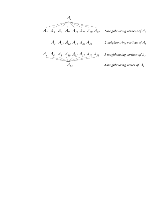
Figure 2: The ”neighborhood structure” of $P_{24}$

Definition 3.1

1. The $1$-neighbouring vertices of $A_{i}$ $(i\in\{1,2,\dots,24\})$ among the vertices of $P_{24}$ are the vertices $A_{j}$ where $A_{i}A_{j}$ is an edge of $P_{24}$.

2. The $2$-neighbouring vertices of $A_{i}$ $(i\in\{1,2,\dots,24\})$ among the vertices of $P_{24}$ are $A_{j}$ where $A_{i}A_{j}$ is a diagonal of an octahedral facet of $P_{24}$.

3. The $4$-neighbouring vertex of $A_{i}$ $(i\in\{1,2,\dots,24\})$ among the vertices of $P_{24}$ is it opposite vertex $A_{j}$ regarding $P_{24}$.

4. The $3$-neighbouring vertices of $A_{i}$ $(i\in\{1,2,\dots,24\})$ among the vertices of $P_{24}$ are the vertices $A_{j}$ that are not $k$-neighbouring $(k=1,2,4)$ vertices of $A_{i}$.

The Fig. 2 shows the $k$-neighbouring vertices $(k=1,2,3,4)$ of $A_{1}$.

Definition 3.2

Two horoballs $B_{i}$ and $B_{j}$ (or horospheres $B_{i}^{s}$ and $B_{j}^{s}$ $(i,j\in\{1,2,\dots,24\},\ \ i\neq j)$ among the horoballs centered at the vertices $P_{24}$ are $k$-neighbouring $(k\in\{1,2,3,4\})$ if their centres $A_{i}$ and $A_{j}$ are $k$-neighbouring vertices regarding $P_{24}$.

We choose a characteristic simplex (orthoscheme) of $P_{24}$ with vertices $T_{0}=A_{1}\Big{(}1,\frac{1}{\sqrt{2}},\frac{1}{\sqrt{2}},$ $0,0\Big{)}$, $T_{1}$, $T_{2}$, $T_{3}$ and $T_{4}=O$ where $T_{4}(1,0,0,0,0)$ is the centre of $P_{24}$ (coincides with the center of the model), $T_{3}\Big{(}1,\frac{1}{2\sqrt{2}},\frac{1}{2\sqrt{2}},\frac{1}{2\sqrt{2}},\frac{1}{2\sqrt{2}}\Big{)}$ is the centre of the facet-polyhedron $A_{1}A_{3}A_{5}A_{7}A_{9}A_{11}$ (octahedron), the centre of its regular face-polygon $A_{1}A_{3}A_{7}$ (regular triangle) is denoted by $T_{2}\Big{(}1,\frac{2}{3\sqrt{2}},\frac{2}{3\sqrt{2}},\frac{2}{3\sqrt{2}},0\Big{)}$ and $T_{1}\Big{(}1,\frac{1}{\sqrt{2}},\frac{1}{2\sqrt{2}},\frac{1}{2\sqrt{2}},0\Big{)}$ is the centre of the edge $A_{1}A_{3}$ of this face. Moreover, we denote by $T\Big{(}1,\frac{1}{2\sqrt{2}},$ $\frac{1}{2\sqrt{2}},\frac{1}{\sqrt{2}},0\Big{)}$ the center of the edge $A_{3}A_{7}$. This point is coincide with the orthogonal projection of $A_{1}$ onto its adjacent octahedral facet $A_{3}A_{4}A_{7}A_{8}A_{11}A_{24}$ (see Fig. 3).

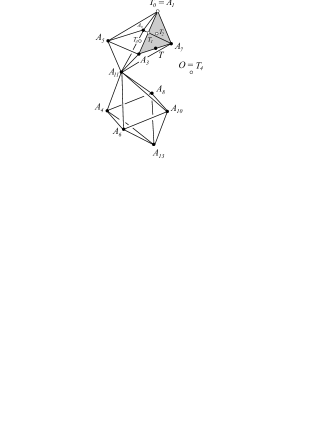
Figure 3: A part of $P_{24}$

4 Horoball packings and polyhedral density function

Similarly to the above section let $P_{24}$ be a tile of the 4-dimensional regular honeycomb $\mathcal{P}_{24}$ with Schläfli symbol $\{3,4,3,4\}$. We study the horoball packings $\mathcal{B}$ with horoballs centred at the infinite vertices of $\mathcal{P}_{24}$. The horospheres and horoball centred at the vertex $A_{i}$ are denoted by $B_{i}^{s}$ and $B_{i}$. The density $\delta(\mathcal{B})$ of the horoball packing $\mathcal{B}$ relating to the above Coxeter tiling can be defined as the extension of the local density related to the polytop $P_{24}$. It is well known that for periodic ball or horoball packings the local density can be extended to the entire hyperbolic space.

Definition 4.1

We consider the polytop $P_{24}$ with vertices $A_{i}$ $(i=1,\dots,24)$ in $4$-dimensional hyperbolic space $\overline{\mathbf{H}}^{4}$. Centres of horoballs lie at vertices of $P_{24}$. We allow horoballs $(B_{i},\leavevmode\nobreak\ i=0,1,2,\dots,24)$ of different types at the various vertices and require to form a packing, moreover we assume that

$$card\Big{[}B_{i}\cap int\Big{\{}\cup_{j=1}^{18}\mathcal{O}_{i_{j}}\Big{\}}\Big{]}=0,$$

where the hyperplanes $\mathcal{O}_{i_{j}}$ $(j=1,\dots,18)$ do not contain the vertex $A_{i}$. The generalized polyhedral density function for the above polytop and horoballs is defined as

$$\delta(\mathcal{B})=\frac{\sum_{i=0}^{24}Vol(B_{i}\cap P_{24})}{Vol(P_{24})}.$$

The aim of this section is to determine the optimal packing arrangements $\mathcal{B}_{opt}$ and their densities for the regular honeycomb $\mathcal{P}_{24}$ in $\overline{\mathbf{H}}^{4}$. We vary the types of the horoballs so that they satisfy our constraints of non-overlap. The packing density is obtained by the above definition.

We will use the consequences of the following Lemma (see [35]):

Lemma 4.2

Let $B_{1}$ and $B_{2}$ denote two horoballs with ideal centers $C_{1}$ and $C_{2}$, respectively, in the $n$-dimensional hyperbolic space $(n\geq 2)$. Take $\tau_{1}$ and $\tau_{2}$ to be two congruent $n$-dimensional convex piramid-like regions, with vertices $C_{1}$ and $C_{2}$. Assume that these horoballs $B_{1}(x)$ and $B_{2}(x)$ are tangent at point $I(x)\in{C_{1}C_{2}}$ and ${C_{1}C_{2}}$ is a common edge of $\tau_{1}$ and $\tau_{2}$. We define the point of contact $I(0)$ (the so-called ,,midpoint”)such that the following equality holds for the volumes of horoball sectors:

$$V(0):=2vol(B_{1}(0)\cap\tau_{1})=2vol(B_{2}(0)\cap\tau_{2}).$$

If $x$ denotes the hyperbolic distance between $I(0)$ and $I(x)$, then the function

$$V(x):=vol(B_{1}(x)\cap\tau_{1})+vol(B_{2}(x)\cap\tau_{2})=\frac{V(0)}{2}(e^{(n-1)x}+e^{-(n-1)x})$$

strictly increases as $x\rightarrow\pm\infty$.

We consider the following four basic horoball configurations $\mathcal{B}_{i}$, $(i=0,1,2,3,4)$:

1. All $24$ horoballs are of the same type and the adjacent horoballs touch each other at the ,,midpoints” of each edge. This horoball arrangement is denoted by $\mathcal{B}_{0}$.

2. We allow horoballs of different types and the opposite horoballs e.g. $B_{1}$ and $B_{13}$ touch their common 2-neighbouring horoballs $B_{i}$ $(i=2,11,12,14,23,$ $24)$ (see Fig. 2) at the centres of the corresponding octahedral facets e.g. the horoball $B_{1}$ touches the horoball $B_{11}$ at the facet center $T_{3}$ and $B_{13}$ tangent $B_{11}$ at the centre of octahedral facet $A_{4}A_{6}A_{8}A_{10}A_{11}A_{13}$ (see Fig. 3). The other ”smaller” horoballs are in the same type regarding $P_{24}$ and touch their 1-neighbouring ”larger” horoballs e.g. the ”larger” horoballs $B_{1}$ and $B_{11}$ touch the ”smaller” horoballs $B_{3},B_{5},B_{7},B_{9}$. At this horoball arrangement let the point $A_{1}A_{3}\cap B_{1}^{s}$ be denoted by $C=I_{1}$ (see Fig. 4.a) ($B_{i}^{s}$ is the corresponding horosphere of horoball $B_{i}$.)

   This horoball arrangement is denoted by $\mathcal{B}_{1}$.

3. We set out from the $\mathcal{B}_{1}$ ball configuration and we expand the horoballs $B_{1}$ and $B_{13}$ until they comes into contact with their adjacent facets regarding $P_{24}$ while keeping their $1$ and $2$-neighbouring horoballs tangent to them. At this configuration which is denoted by $\mathcal{B}_{2}$ the horoballs are included on $3$ classes related to $P_{24}$. The horoballs $B_{1}$ and $B_{13}$ are in the same type and they touch their corresponding $1$-neighbouring horoballs that form the second class. The remaining $8$ horoballs are also in same type and are included on the $3$. type.

   For example the horoball $B_{1}$ touches its neighbouring facet at the point $T$ (see Fig. 3, and Fig. 4.b) and touches its $1$-neighbouring horoballs e.g. $B_{3},B_{5},B_{7},B_{9}$ and its $2$-neighbouring horoballs e.g. $B_{11}$. At this horoball arrangement let the point $A_{1}A_{11}\cap B_{1}^{s}$ be denoted by $E=I_{3}$ (see Fig. 4.b).

4. We set out also from the $\mathcal{B}_{1}$ ball configuration and we expand the horoball $B_{1}$ until they comes into contact with their adjacent facets regarding $P_{24}$ while keeping their $1$ and $2$-neighbouring horoballs tangent to them. Moreover, we ”blow up” the $3$-neighbouring horoballs of $B_{1}$ while their $1$-neighbouring horoballs touch them. At this configuration e.g. the horoball $B_{1}$ touches its neighbouring facet $A_{3}A_{4}A_{7}A_{8}A_{11}A_{24}$ at the point $T$ (see Fig. 3, and Fig. 4.b) and touch its $1$-neighbouring horoballs e.g. $B_{3},B_{5},B_{7},B_{9}$ and its $2$-neighbouring horoballs e.g. $B_{11}$. Furthermore, the ”expanded” horoballs e.g. $B_{4},B_{6},B_{8},B_{10}$ touch the ”shrunk” horoballs $B_{11}$ and $B_{13}$.

   This horoball arrangement is denoted by $\mathcal{B}_{3}$.

5. Now we start from the configuration $\mathcal{B}_{0}$ and we choose three arbitrary, mutually $3$-neighbouring horoballs and expand them until they comes into contact with each other while keeping their $1$-neighbouring horoballs tangent to them. We note here that this horoball configuration can be realized in $\mathbf{H}^{4}$ (see the subsection 4.2.4). At this configuration which is denoted by $\mathcal{B}_{4}$ the horoballs are included on $2$ classes related to $P_{24}$, e.g. the horoballs $B_{1}$, $B_{10}$, $B_{17}$ are in same type touching each other and their ”smaller” $1$-neighbouring horoballs that are also in same type.

4.1 Optimal horoball packings with horoballs in same type

In this Section we consider the packings of horoballs where $Vol(B_{i}\cap P_{24})=Vol(B_{j}\cap P_{24})$ for all $i,j\in\{1,2,\dots,24\}$ thus the horoballs $B_{i}$ are in the same type regarding $P_{24}$.

It is clear that in this case the maximal density can be achieved if the neighbouring horoballs touch each other at the centres of the edges of $P_{24}$ and the density of this densest packing $\mathcal{\mathcal{B}}_{0}$ is equal to the maximal density of the horoball packings related to the Coxeter simplex tiling $\{3,4,3,4\}$. For example in this case two horoballs $B_{1}$ and $B_{3}$ touch at the ”midpoint” $T_{1}$ of edge $A_{1}A_{3}$ as projection of the polyhedron centre on it (see Fig. 3). These ball packings were investigated by the author in [27]:

$$\begin{gathered}V_{0}:=Vol(B_{i}\cap\mathcal{F}_{24})=\frac{1}{216}\sqrt{2}\sinh{\Big{(}\frac{1}{2}\mathrm{arcosh}{\Big{(}\frac{11}{8}\Big{)}}\Big{)}}\approx 0.00694,\\ Vol(\mathcal{F}_{24})=\frac{\pi^{2}}{864},\ \ \delta(\mathcal{B}_{0})=\frac{Vol(B_{i}\cap\mathcal{F}_{24})}{Vol(\mathcal{F}_{24})}\approx 0.60793.\end{gathered}$$ (4.1)

4.2 Optimal horoball packings with horoballs in different types

The type of a horoball is allowed to expand until either the horoball comes into contact with other horoballs or with a adjacent facet of the honeycomb. These conditions are satisfactory to ensure that the balls form a non-overlapping horoball arrangement, as such the collection of all horoballs is a well defined packing in $\mathbb{H}^{4}$.

4.2.1 Horoball packings $\mathcal{B}_{0}^{1}$ and their densities between the horoball arrangements $\mathcal{B}_{0}$ and $\mathcal{B}_{1}$

We set out from the $\mathcal{B}_{0}$ ball configuration (see above Section) and consider two $1$-neighbouring horoballs e.g. $B_{1}$ and $B_{3}$ from it. Let $I_{0}=I(0)=T_{1}$ be their point of tangency on side $A_{1}A_{3}$ (see Fig. 3 and Fig. 4.a). Moreover, consider the point $I(x)$ on the segment $A_{1}A_{3}$ where the modified horoballs $B_{i}(x),\ (i=1,3)$ are tangent to each other and $x$ is the hyperbolic distance between $I(0)$ and $I(x)$ (the value of $x$ can also be negative if $I(x)$ is on the segment $T_{1}A_{1}$).

We blow up the horoballs $B_{1}(0)$ and $B_{11}(0)$ (and also the horoballs $B_{2}$, $B_{12}$, $B_{14}$, $B_{23}$, $B_{24}$ and $B_{13}$ to achieve the $\mathcal{B}_{1}$ horoball configuration) until they come into contact with each other at the centre $T_{3}$ of octahedral facet $A_{1}A_{3}A_{5}A_{7}A_{9}A_{11}$. At this situation (see Fig. 3) the horoball centered at $A_{1}$ is denoted, by $B_{1}(\rho_{1})$ where $\rho_{1}$ is the hyperbolic distance between $I_{0}$ and $I_{1}$ (see Fig. 4.a).

The foot-point of the perpendicular from $T_{3}$ onto the staight line $A_{1}A_{3}$ is $I_{0}=T_{1}$ which is the common point of the horoballs $B_{1}(0)\in\mathcal{B}_{0}$ and $B_{3}(0)\in\mathcal{B}_{0}$ centered at $A_{1}$ and $A_{3}$, respectively. The hyperbolic distance $s_{1}=T_{1}T_{3}$ between the points $T_{1}[\mathbf{t}_{1}]$ and $T_{3}[\mathbf{t}_{3}]$ can be computed by the formula (2.5) (see Fig. 4.a):

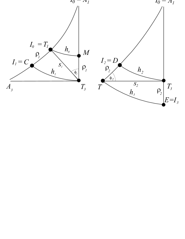
a.                                             b.

Figure 4: Computations of hyperbolic distances $\rho_{1}=I_{0}I_{1}$ and $\rho_{2}=I_{2}T=I_{3}T_{3}$

The parallel distance of the angle $\phi_{1}=T_{1}T_{3}A_{1}\angle$ is $s_{1}$ therefore we obtain by the classical formula of J. Bolyai and by formula (2.5) the following equation (see Fig. 4.a).

$$\frac{1}{\sin{(\phi_{1}})}=\cosh{s_{1}}=\sqrt{2}.$$ (4.2)

We consider two horocycles $\mathcal{H}_{0}$ and $\mathcal{H}_{1}$ through the points $I_{0}$ and $I_{1}$ with center $A_{1}$ in the plane $A_{1}A_{3}T_{3}$ and the point $\mathcal{H}_{1}\cap A_{1}T_{3}$ is denoted by $M$. The horocyclic distances between points $I_{0}$, $M$ and $I_{1}$, $T_{3}$ are denoted by $h_{0}$ and $h_{1}$. By means of formula of J. Bolyai and of (4.2), we have

$$\begin{gathered}\frac{h_{1}}{h_{0}}=e^{\rho_{1}}=\frac{1}{\sin(\phi_{1})}\ \Rightarrow\rho_{1}=\log(\sqrt{2})\approx 0.34657.\end{gathered}$$ (4.3)

We extend the above modifications and denotations for all horoballs of packings between horoball arrangements $\mathcal{B}_{0}$ and $\mathcal{B}_{1}$ i.e. the horoballs are denoted by $B_{i}(x)$ $(i\in[0,\rho_{1}])$. If $x=0$ then we get the $\mathcal{B}_{0}$ horoball packing and if $x=\rho_{1}$ then the $\mathcal{B}_{1}$ one.

We obtain using the results of the former computations and of Lemma 4.2 the next

Lemma 4.3

The density of packings $\mathcal{B}_{0}^{1}$ (see Fig. 5.a) between the main horoball arrangements $\mathcal{B}_{0}$ and $\mathcal{B}_{1}$ can be computed by the formula

$$\begin{gathered}\delta(\mathcal{B}_{0}^{1}(x))=\frac{\sum_{i=0}^{24}Vol(B_{i}(x)\cap P_{24})}{Vol(P_{24})}=\frac{384\cdot V_{0}\leavevmode\nobreak\ (e^{3x}+2\cdot e^{-3x})}{\frac{4}{3}\pi^{2}},\leavevmode\nobreak\ \leavevmode\nobreak\ x\in[0,\rho_{1}]\end{gathered}$$

and the maxima of function $\delta(\mathcal{B}_{0}^{1}(x))$ (see Fig. 5.a) are realized at $x=\rho_{1}\leavevmode\nobreak\ \approx 0.34657$ where the horoball packing density is $\delta(\mathcal{B}_{0}^{1}(\rho_{1}))\approx 0.71645$.

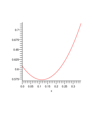
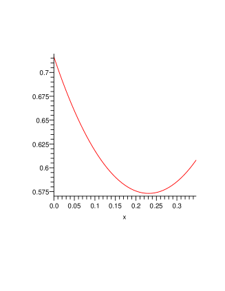
a.                                             b.

Figure 5: The graphs of functions $\delta(\mathcal{B}_{0}^{1}(x))$ and $\delta(\mathcal{B}_{1}^{2}(x))$ where $x\in[0,\rho_{1}]$.

Remark 4.4

We note, here that the above optimal density $\delta(\mathcal{B}_{0}^{1}(\rho_{1}))\approx 0.71645$ is equal to the density of known densest ball and horoball packings in $\mathbb{H}^{4}$.

4.2.2 Horoball packings $\mathcal{B}_{1}^{2}$ and their densities between the horoball arrangements $\mathcal{B}_{1}$ and $\mathcal{B}_{2}$

We start our investigation from the $\mathcal{B}_{1}$ ball configuration. Here e.g. the horoballs $B_{1}$ and $B_{3}$ touch each other at the point $I_{1}$ (see Fig. 4.a) and $B_{1}$ touch $B_{11}$ at the point $T_{3}$ (see Fig. 3 and Fig. 4.b) etc. Furthermore, in $\mathcal{B}_{1}$ the common point of horosphere $B_{1}^{s}$ with the line segment $A_{1}T$ is denoted by $I_{2}=I^{*}(0)=D$ (see Fig. 4.b). We consider the point $I^{*}(x)$ on the segment $A_{1}T$ where a modified horosphere $B_{1}^{s}(x)$ intersects the line segment $A_{1}T$ and $x$ is the hyperbolic distance between $I^{*}(0)$ and $I^{*}(x)$ (the value of $x$ can also be negative if $I^{*}(x)$ is on the segment $A_{1}I^{*}(0)$). Corresponding to the above notions we introduce the notations $B_{13}(0)$ and $B_{13}(x)$.

We blow up the horoballs $B_{1}(0)$ and $B_{13}(0)$ while keeping their $1$-neighbouring horoballs tangent to them until they comes into contact with their adjacent facets of $P_{24}$ e.g. upto the horoball $B_{1}(x)$ touches the octahedral facet $A_{3}A_{4}A_{7}A_{8}A_{11}A_{24}$. At this arrangement relating to Fig. 4.b the horoball centered at $A_{1}$ is denoted, by $B_{1}(\rho_{2})$ where $\rho_{2}$ is the hyperbolic distance between $I^{*}(0)$ and $T$.

The foot-point of the perpendicular from $T$ onto the staight line $A_{1}A_{11}$ is $T_{3}$. The hyperbolic distance $s_{2}=TT_{3}$ between the point $T[\mathbf{t}]$ and $T_{3}[\mathbf{t}_{1}]$ can be computed by the formula (2.5) (see Fig. 4.b): The parallel distance of the angle $\phi_{2}=A_{1}TT_{3}\angle$ is $s_{2}$ therefore we obtain by the classical formula of J. Bolyai and by formula (2.5) the following equation (see Fig. 4.b):

$$\frac{1}{\sin{(\phi_{2}})}=\cosh{s_{2}}=\sqrt{2}.$$ (4.4)

We consider two horocycles $\mathcal{H}_{2}$ and $\mathcal{H}_{3}$ through the points $I_{2}$ and $T$ with center $A_{1}$ in the plane $A_{1}TT_{3}$ and the point $\mathcal{H}_{3}\cap A_{1}T_{3}$ is denoted by $E=I_{3}$. The horocyclic distances between points $I_{2}$, $T_{3}$ and $T$, $E$ are denoted by $h_{2}$ and $h_{3}$. Similarly to (4.3) we obtain that $\rho_{2}=\log(\sqrt{2})\approx 0.34657$.

We extend the above modifications and denotations for all horoballs of packings between horoball arrangements $\mathcal{B}_{1}$ and $\mathcal{B}_{2}$ i.e. the horoballs are denoted by $B_{i}(x)$ $(i\in[0,\rho_{2}])$. If $x=0$ then we get the $\mathcal{B}_{1}$ horoball packing and if $x=\rho_{2}$ then the $\mathcal{B}_{2}$ one.

We obtain using the results of the former computations and of Lemma 4.2 the next

Lemma 4.5

The density of packings $\mathcal{B}_{1}^{2}$ (see Fig. 5.b) between the main horoball arrangements $\mathcal{B}_{1}$ and $\mathcal{B}_{2}$ can be computed by the formula

$$\begin{gathered}\delta(\mathcal{B}_{1}^{2}(x))=\frac{\sum_{i=0}^{24}Vol(B_{i}(x)\cap P_{24})}{Vol(P_{24})}=\\ =\frac{48\cdot V_{0}\leavevmode\nobreak\ (2\leavevmode\nobreak\ e^{3(\rho_{1}+x)}+6\cdot e^{-3(-\rho_{1}+x)}+16\cdot e^{-3(\rho_{1}+x)})}{\frac{4}{3}\pi^{2}},\leavevmode\nobreak\ \leavevmode\nobreak\ x\in[0,\rho_{2}]\end{gathered}$$

and the maxima of function $\delta(\mathcal{B}_{1}^{2}(x))$ (see Fig. 5.b) are realized at $x=0$ i.e. at the $\mathcal{B}_{1}$ ball packing (see Lemma 4.3).

Remark 4.6

The density $\delta(\mathcal{B}_{1}^{2}(\rho_{2}))$ is equal to the maximal density of packing with horoballs in same types: $\delta(\mathcal{B}_{1}^{2}(\rho_{2}))=\delta(\mathcal{B}_{0})\approx 0.60793$.

4.2.3 Horoball packings $\mathcal{B}_{1}^{3}$ and their densities between the horoball arrangements $\mathcal{B}_{1}$ and $\mathcal{B}_{3}$

Similarly to the above subsection we set out from the $\mathcal{B}_{1}$ ball configuration and we will use the notations of subsection 4.2.2. Now, we expand the horoball $B_{1}(0)$ until they comes into contact with their adjacent facets regarding $P_{24}$ while keeping their $1$ and $2$-neighbouring horoballs tangent to them. Moreover, we ”blow up” the $3$-neighbouring horoballs of $B_{1}(0)$ while their $1$-neighbouring horoballs touch them. At this procedure this horoball is denoted by $B_{1}(x)$. If we achieved the endpoint of this extension then e.g. the horoball $B_{1}(\rho_{2})$ touches its neighbouring facet $A_{3}A_{4}A_{7}A_{8}A_{11}A_{24}$ at the point $T$ (see Fig. 3, and Fig. 4) and touch its $1$-neighbouring horoballs e.g. $B_{3},B_{5},B_{7},B_{9}$ and its $2$-neighbouring horoballs e.g. $B_{11}$. Furthermore, the ”expanded” horoballs e.g. $B_{4},B_{6},B_{8},B_{10}$ touch the ”shrunk” horoballs $B_{11}$ and $B_{13}$.

We extend the above modifications and notations for all horoballs of packings between horoball arrangements $\mathcal{B}_{1}$ and $\mathcal{B}_{3}$ i.e. the horoballs are denoted by $B_{i}(x)$ $(i\in[0,\rho_{2}])$. If $x=0$ then we get the $\mathcal{B}_{1}$ horoball packing and if $x=\rho_{2}$ then the $\mathcal{B}_{3}$ one. Finally, we obtain the next

Lemma 4.7

The density of packings $\mathcal{B}_{1}^{3}$ between the main horoball arrangements $\mathcal{B}_{1}$ and $\mathcal{B}_{3}$ can be computed by the formula

$$\begin{gathered}\delta(\mathcal{B}_{1}^{3}(x))=\frac{\sum_{i=0}^{24}Vol(B_{i}(x)\cap P_{24})}{Vol(P_{24})}=\\ =\frac{48\cdot V_{0}\leavevmode\nobreak\ (e^{3(\rho_{1}+x)}+7\cdot e^{-3(-\rho_{1}+x)}+8\cdot e^{-3(\rho_{1}+x)}+8\cdot e^{-3(\rho_{1}-x)})}{\frac{4}{3}\pi^{2}},\leavevmode\nobreak\ x\in[0,\rho_{2}]\end{gathered}$$

and the maxima of function $\delta(\mathcal{B}_{1}^{3}(x))$ are realized at $x=0$ i.e. at the $\mathcal{B}_{1}$ ball packing (see Lemma 4.3).

Remark 4.8

The function $\delta(\mathcal{B}_{1}^{3}(x))$ is the same with $\delta(\mathcal{B}_{1}^{2}(x))$ $(x\in[0,\rho_{2}])$ (see Fig. 5.b).

4.2.4 Horoball packings $\mathcal{B}_{0}^{4}$ and their densities between the horoball arrangements $\mathcal{B}_{0}$ and $\mathcal{B}_{4}$

Here we consider the horoball configuration $\mathcal{B}_{0}$ and we choose three arbitrary, mutually $3$-neighbouring horoballs e.g. $B_{1}$, $B_{10}$ and $B_{17}$ and let $I_{6}=I_{*}(0)$ be the point of intersection of horosphere $B_{1}^{s}(0)$ with the segment $TA_{1}$. Moreover, consider the point $I_{*}(x)$ on the segment $I_{6}T$ where the expanded horosphere $B_{1}^{s}(x)$ intersects the segment $I_{6}T$ and $x$ is the hyperbolic distance between $I_{*}(0)$ and $I_{*}(x)$ (see Fig. 6.a). We have seen in former subsections that the hyperbolic distance between $I_{0}$ and $T$ is $2\rho_{1}=2\rho_{2}$ (see Fig. 5a and Fig. 5b). We consider a horocycles $\mathcal{H}_{5}$ through the point $T$ with center $A_{1}$ in the plane $A_{1}A_{10}T$ and the point $\mathcal{H}_{5}\cap A_{1}A_{10}$ is denoted by $K=I_{5}$.

The foot-point of the perpendicular from $T$ onto the staight line $A_{1}A_{10}$ is called by $Q$ whose coordinates are $Q\Big{(}1,\frac{5}{7\sqrt{2}},\frac{3}{7\sqrt{2}},0,\frac{2}{7\sqrt{2}}\Big{)}$.

We obtain by in the subsections 4.2.1 and 4.2.2 described method that the hyperbolic distance $\rho_{3}$ of the points $Q$ and $K$ is $\rho_{3}=\log{\frac{10}{3}}$.

The centre (”midpoint”) of segment $A_{1}A_{10}$ is denoted by $H$ (see Fig. 6.a) (in our model this is Euclidean midpoint of segment $A_{1}A_{10}$, as well) whose distance $\rho_{4}$ to $Q$ can be computed by the formula (2.5): $\rho_{4}={\text{arccosh}}\Big{(}\frac{7\sqrt{2}}{4\sqrt{5}}\Big{)}$. The point $H$ lie on the line segment $QK$ because $0.60199\approx\rho_{3}>\rho_{4}\approx 0.45815$.

Finally, we obtain using the results of the former computations and of Lemma 4.2 the next

Lemma 4.9

The density of packings $\mathcal{B}_{0}^{4}$ (see Fig. 5.b) between the main horoball arrangements $\mathcal{B}_{0}$ and $\mathcal{B}_{4}$ can be computed by the formula

$$\begin{gathered}\delta(\mathcal{B}_{0}^{4}(x))=\frac{\sum_{i=0}^{24}Vol(B_{i}(x)\cap P_{24})}{Vol(P_{24})}=\\ =\frac{48\cdot V_{0}\leavevmode\nobreak\ (3\cdot e^{3x}+21\cdot e^{-3x})}{\frac{4}{3}\pi^{2}},\leavevmode\nobreak\ \leavevmode\nobreak\ x\in[0,2\rho_{1}+\rho_{4}-\rho_{3}\approx 0.54931]\end{gathered}$$

and the maxima of function $\delta(\mathcal{B}_{0}^{4}(x))$ (see Fig. 6.b) are realized at $x=0$ where the horoball packing density is $\delta(\mathcal{B}_{0}^{4}(0))\approx 0.60793$.

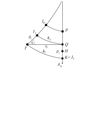
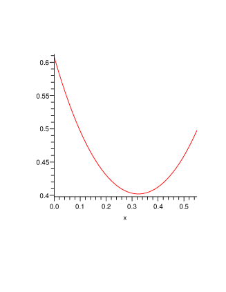
a.                                             b.

Figure 6: a. The computation of hyperbolic distance $\rho_{3}=I_{4}T$ and $\rho_{4}=QH$.  b.  The graph of function $\delta(\mathcal{B}_{0}^{4}(x))$ $x\in[0,2\rho_{1}+\rho_{3}-\rho_{4}]$.

Remark 4.10

The density $\delta(\mathcal{B}_{0}^{4}(0))$ is equal to the maximal density of packings with horoballs in same types: $\delta(\mathcal{B}_{0}^{4}(\rho_{2}))=\delta(\mathcal{B}_{0})\approx 0.60793$.

4.3 Optimal horoball packings to hyperbolic $24$-cell

The main result of this paper is summarized in the following

Theorem 4.11

The horoball arrangement $\mathcal{B}_{1}$ (see 4.2.1) provide the maximal horoball packing density related to the hyperbolic tiling $\mathcal{P}_{24}$ with Schläfli symbol $\{3,4,3,4\}$ and its density is $\delta_{opt}(\mathcal{B})\approx 0.71645$ if horoballs of different types are allowed at each asymptotic vertex of the tiling.

Remark 4.12

The optimal horoball packing described and determined in this paper is a new horoball configuration which provide the known maximal density of realizable packings of the entire hyperbolic space $\mathbb{H}^{4}$.

Proof

It is well known that a packing is optimal, then it is locally stable i.e. each ball is fixed by the other ones so that no ball of packing can be moved alone without overlapping another ball of the given ball packing.

The packings of horoballs can be easily classified by the type of ”maximally large” horoball regarding the horoball packing to $\mathcal{P}_{24}$. If we fix the ”maximally large” horoball related to the above tiling then all possible horoball packing can be modified to achieve one of the above horoball configurations $\mathcal{B}_{i}^{j}(x)$ $(i,j\in{\{0,1,2,3,4\}},\leavevmode\nobreak\ i<j)$ without decrease of the packing density.

A horoball $B_{i}(x)$ is ”maximally large” if $Vol(B_{i}(x)\cap P_{24})$ $(i\in 1\dots 24)$ is maximal. Here the maximal volume is denoted by $Vol(B_{i}^{max})$.

1. If $\frac{1}{48}Vol(B_{i}^{max})\leq V_{0}$ then the maximal density can be computed by Sect. 4.1 where the maximal density is $\delta(\mathcal{B}_{0})\approx 0.60793$.

2. If $V_{0}<\frac{1}{48}\cdot Vol(B_{i}^{max})\leq V_{0}\cdot e^{3\rho_{1}}$ then the optimal density can be computed by Sections 4.2.1, here the optimal density is $\delta(\mathcal{B}_{0}^{1}(\rho_{1}))\approx 0.71645$.

3. If $V_{0}\cdot e^{3\rho_{1}}<\frac{1}{48}\cdot Vol(B_{i}^{max})\leq V_{0}\cdot e^{6\rho_{1}}$ then the densities can be computed by Sections 4.2.2, 4.2.3 and 4.2.4 where the maximal density is $\delta(\mathcal{B}_{0})\approx 0.60793$.

The volume of the ”largest horoball” $Vol(B_{i}^{max})\leq V_{0}\cdot e^{6\rho_{1}}$ therefore we proved the above Theorem. $\square$

The above results also show, that the discussion of the densest horoball packings and coverings in the $n$-dimensionalen hyperbolic space with horoballs of different types has not been settled yet. Similarly to these, the problems of the densest hypersphere (or hyperball) packings and coverings are open, as well.

Optimal sphere packings in other homogeneous Thurston geometries form also a class of open mathematical problems (see [28], [29], [30], [31], [32], [33], [16], [17], [18]). Detailed studies are the objective of ongoing research.

References

- [1] Bezdek, K. Sphere Packings Revisited, European Journal of Combinatorics (2006) 27/6 , 864–883.
- [2] Bowen, L. - Radin, C. Optimally Dense Packings of Hyperbolic Space, Geometriae Dedicata, (2004) 104 , 37–59.
- [3] Böhm, J. - Hertel, E. Polyedergeometrie in -dimensionalen Räumen konstanter Krümmung, Birkhäuser, Basel (1981).
- [4] Böröczky, K. Packing of spheres in spaces of constant curvature, Acta Math. Acad. Sci. Hungar., (1978) 32 , 243–261.
- [5] Böröczky, K. - Florian, A. Über die dichteste Kugelpackung im hyperbolischen Raum, Acta Math. Acad. Sci. Hungar., (1964) 15 , 237–245.
- [6] Coxeter, H. S. M. Regular honeycombs in hyperbolic space, Proceedings of the International Congress of Mathematicians, Amsterdam, (1954) III , 155–169.
- [7] Fejes Tóth, G. - Kuperberg, G. - Kuperberg, W. Highly Saturated Packings and Reduced Coverings, Monatshefte für Mathematik, (1998) 125/2, 127–145.
- [8] Johnson, N. W. – Kellerhals, R. – Ratcliffe, J. G. and Tschantz, S. T. The size of a hyperbolic Coxeter simplex, Transformation Groups (1999) 4/4 , 329–353.
- [9] Kellerhals, R. Ball packings in spaces of constant curvature and the simplicial density function, Journal für reine und angewandte Mathematik, (1998) 494 , 189–203.
- [10] Kellerhals, R. Regular simplices and lower volume bounds for hyperbolic -manifolds, Ann. Global Anal. Geom., (1995) 13 , 377–392.
- [11] Kolpakov, A. On the optimality of the ideal right-angled 24 cell, Algebr. Geom. Topol., (2012) 12/4 , 1941–1960.
- [12] Kozma, T. R. - Szirmai, J. Optimally dense packings for fully asymptotic Coxeter tilings by horoballs of different types, Monatshefte für Mathematik, (2012) 168 , 27–47, DOI: 10.1007/s00605-012-0393-x.
- [13] Kozma, T. R. - Szirmai, J. New Lower Bound for the Optimal Ball Packing Density of Hyperbolic 4-space, Discrete Comput. Geom., (2015) 53, 182–198, DOI: 10.1007/s00454-014-9634-1.
- [14] Molnár, E. The projective interpretation of the eight 3-dimensional homogeneous geometries, Beitr. Algebra Geom., (1997) 38/2, 261–288.
- [15] Molnár, E. - Prok, I. - Szirmai, J. Classification of tile-transitive 3-simplex tilings and their realizations in homogeneous spaces. A. Prékopa and E. Molnár, (eds.). Non-Euclidean Geometries, János Bolyai Memorial Volume, Mathematics and Its Applications, Springer (2006) Vol. 581, 321-363.
- [16] Molnár, E. – Szirmai, J. Volumes and geodesic ball packings to the regular prism tilings in space. Publ. Math. Debrecen, 84/1-2 (2014), 189-203, DOI: 10.5486/PMD.2014.5832.
- [17] Molnár, E. – Szirmai, J. – Vesnin, A. Packings by translation balls in . J. Geometry 105/2 (2014), 287-306, DOI: 10.1007/s00022-013-0207-x.
- [18] Molnár, E. – Szirmai, J. – Vesnin, A. Geodesic and translation ball packings generated by prismatic tesselations of the universal cover of . Submitted Manuscript
- [19] Marshall, T. H. Asymptotic Volume Formulae and Hyperbolic Ball Packing, Annales Academiæ Scientiarum Fennicæ: Mathematica, (1999) 24, 31–43.
- [20] Milnor, J. Geometry, Collected papers, Publish or Perish, (1994) Vol 1.
- [21] Radin, C. The symmetry of optimally dense packings, A. Prékopa and E. Molnár, (eds.). Non-Euclidean Geometries, János Bolyai Memorial Volume, Mathematics and Its Applications, Springer (2006) Vol. 581, 197-207.
- [22] Ratcliffe, J. G. and Tschantz, S. T. The volume spectrum of hyperbolic 4-manifolds, Experiment. Math. (2000) 9/1 , 101–125.
- [23] Rogers, C. A. Packing and covering, Cambridge University Press, (1964).
- [24] Slavich, L. Some hyperbolic 4-manifolds with low volume and number of cusps, Manuscript (2014) http://arxiv.org/abs/1402.2580
- [25] Szirmai, J. Horoball packings for the Lambert-cube tilings in the hyperbolic 3-space, Beitr. Algebra Geom., (2005) 46/1, 43-60.
- [26] Szirmai, J. The optimal ball and horoball packings of the Coxeter tilings in the hyperbolic -space, Beitr. Algebra Geom., (2005) 46/2, 545–558.
- [27] Szirmai, J. The optimal ball and horoball packings to the Coxeter honeycombs in the hyperbolic -space, Beitr. Algebra Geom., (2007) 48/1, 35–47.
- [28] Szirmai, J. The densest geodesic ball packing by a type of lattices, Beitr. Algebra Geom., (2007) 48/2, 383–397.
- [29] Szirmai, J. The densest translation ball packing by fundamental lattices in space, Beitr. Algebra Geom., (2010) 51/2, 353–373.
- [30] Szirmai, J. Geodesic ball packing in space for generalized Coxeter space groups, Beitr. Algebra Geom., (2011) 52, 413–430.
- [31] Szirmai, J. Geodesic ball packing in space for generalized Coxeter space groups. Math. Commun., 17/1 (2012), 151-170.
- [32] Szirmai, J. Lattice-like translation ball packings in space. Publ. Math. Debrecen, 80/3-4 (2012), 427–440, DOI: 10.5486/PMD.2012.5117.
- [33] Szirmai, J. A candidate to the densest packing with equal balls in the Thurston geometries. Beitr. Algebra Geom., 55/2 (2014), 441- 452, DOI 10.1007/s13366-013-0158-2.
- [34] Szirmai, J. Horoball packings and their densities by generalized simplicial density function in the hyperbolic space, Acta Math. Hungar., (2012) 136/1-2, 39–55, DOI: 10.1007/s10474-012-0205-8.
- [35] Szirmai, J. Horoball packings to the totally asymptotic regular simplex in the hyperbolic -space, Aequat. Math., 85 (2013), 471–482, DOI: 10.1007/s00010-012-0158-6.