Discriminative training for Convolved Multiple-Output Gaussian processes

Abstract

Multi-output Gaussian processes (MOGP) are probability distributions over vector-valued functions, and have been previously used for multi-output regression and for multi-class classification. A less explored facet of the multi-output Gaussian process is that it can be used as a generative model for vector-valued random fields in the context of pattern recognition. As a generative model, the multi-output GP is able to handle vector-valued functions with continuous inputs, as opposed, for example, to hidden Markov models. It also offers the ability to model multivariate random functions with high dimensional inputs. In this report, we use a discriminative training criteria known as Minimum Classification Error to fit the parameters of a multi-output Gaussian process. We compare the performance of generative training and discriminative training of MOGP in emotion recognition, activity recognition, and face recognition. We also compare the proposed methodology against hidden Markov models trained in a generative and in a discriminative way.

1 Introduction

A growing interest within the Gaussian processes community in Machine learning has been the formulation of suitable covariance functions for describing multiple output processes as a joint Gaussian process. Examples include the semiparametric latent factor model Teh et al. (2005), the multi-task Gaussian process Bonilla et al. (2008), or the convolved multi-output Gaussian process Boyle and Frean (2005); Álvarez and Lawrence (2009). Each of these methods uses as a model for the covariance function either a version of the linear model of coregionalization (LMC) Goovaerts (1997) or a version of process convolutions (PC) Higdon (2002). Different alternatives for building covariance functions for multiple-output processes have been reviewed by Álvarez et al. (2012).

Multiple output GPs have been used for supervised learning problems, specifically, for multi-output regression Bonilla et al. (2008), and multi-class classification Skolidis and Sanguinetti (2011); Chai (2012). The interest has been mainly on exploiting the correlations between outputs to improve the prediction performance, when compared to modeling each output independently. In particular, a Gaussian process is used as a prior over vector-valued functions $\mathbf{f}(\mathbf{x})$ mapping from $\mathbf{x}\in\mathbb{R}^{p}$ to $\mathbf{f}\in\mathbb{R}^{D}$. Components of $\mathbf{f}$ may be continuous or discrete.

In this report, we advocate the use of multi-output GPs as generative models for vector-valued random fields, this is, we use multi-output GPs to directly modeling $p(\mathbf{f}(\mathbf{x}))$. Afterwards, we use this probabilistic model to tackle a classification problem. An important application area where this setup is of interest is in multivariate time series classification. Here the vector-valued function $\mathbf{f}$ is evaluated at discrete values of $\mathbf{x}$, and it is typically modeled using an unsupervised learning method like a hidden Markov model (HMM) or a linear dynamical system (LDS) Bishop (2007). Notice that by using a multi-output GP to model $\mathbf{f}(\mathbf{x})$, we allow the vector-valued function $\mathbf{f}(\mathbf{x})$ to be continuous on the input space. Furthermore, we are able to model multivariate random functions for which $p>1$. It is worth mentioning that the model we propose here, is different from classical GP classification as explained for example in Rasmussen and Williams (2006). In standard GP classification, the feature space is not assumed to follow a particular structure, whereas in our model, the assumption is that the feature space may be structured, with potentially correlated and spatially varying features.

As a generative model, the multi-output Gaussian process can be used for classification: we fit a multi-output GP for every class independently, and to classify a new vector-valued random field, we compute its likelihood for each class and make a decision using Bayes rule. This generative approach works well when the real multivariate signal’s distribution is known, but this is rarely the case. Notice that the optimization goal in the generative model is not a function that measures classification performance, but a likelihood function that is optimized for each class separately.

An alternative is to use discriminative training Jebara (2004) for estimating the parameters of the multi-output GP. A discriminative approach optimizes a function classification performance directly. Thus, when the multi-output GP is not an appropriate generative distribution the results of the discriminative training procedure are usually better. There are different criteria to perform discriminative training, including maximum mutual information (MMI) Gopalakrishnan et al. (1991), and minimum classification error (MCE) Juang et al. (1997).

In this report we present a discriminative approach to estimate the hyperparameters of a multi-output Gaussian Process (MOGP) based on minimum classification error (MCE). In section 2 we review how to fit the multi-output GP model using the generative approach, and then we introduce our method to train the same MOGP model with a discriminative approach based on MCE. In section 3 we show experimental results, with both the generative and discriminative approaches. Finally, we present conclusions on section 4.

2 Generative and discriminative training of multi-output GPs

In our classification scenario, we have $M$ classes. We want to come up with a classifier that allows us to map the matrix $\mathbf{F}(\mathbf{X})$ to one of the $M$ classes. Columns of matrix $\mathbf{X}$ are input vectors $\mathbf{x}_{n}\in\mathbb{R}^{p}$, and columns of matrix $\mathbf{F}$ are feature vectors $\mathbf{f}({\mathbf{x}}_{n})\in\mathbb{R}^{D}$, for some $n$ in an index set. Rows for $\mathbf{F}$ correspond to different entries of $\mathbf{f}({\mathbf{x}}_{n})$ evaluated for all $n$. For example, in a multi-variate time series classification problem, $\mathbf{x}_{n}$ is a time point $t_{n}$, and $\mathbf{f}({\mathbf{x}}_{n})$ is the multi-variate time series at $\mathbf{x}_{n}=t_{n}$. Rows of the matrix $\mathbf{F}$ are the different time series.

The main idea that we introduce in this report is that we model the class-conditional density $p(\mathbf{F}|\mathbf{X},\mathcal{C}_{m},\bm{\theta}_{m})$ using a multi-output Gaussian process, where $\mathcal{C}_{m}$ is the class $m$, and $\bm{\theta}_{m}$ are hyperparameters of the multi-output GP for class $m$. By doing so, we allow correlations across the columns of $\mathbf{F}$, this is between $\mathbf{f}({\mathbf{x}}_{n})$ and $\mathbf{f}({\mathbf{x}}_{m})$, for $n\neq m$, and also allow correlations among the variables in the vector $\mathbf{f}({\mathbf{x}}_{n})$, for all $n$. We then estimate $\bm{\theta}_{m}$ for all $m$ in a generative classification scheme, and in a discriminative classification scheme using minimum classification error. Notice that a HMM would model $p(\mathbf{F}|\mathcal{C}_{m},\bm{\theta}_{m})$, since vectors $\mathbf{f}_{n}$ would be already defined for discrete values of ${\mathbf{x}}$. Also notice that in standard GP classification, we would model $p(\mathcal{C}_{m}|\mathbf{F})$, but with now particular correlation assumptions over the entries in $\mathbf{F}$.

Available data for each class are matrices $\mathbf{F}_{m}^{l}$, where $m=1,\ldots,M$, and $l=1,\ldots,L_{m}$. Index $\l$ runs over the instances for a class, and each class has $L_{m}$ instances. In turn, each matrix $\mathbf{F}_{m}^{l}\in\mathbb{R}^{D\times N_{m}^{l}}$ with columns $\mathbf{f}_{m}^{l}({\mathbf{x}_{n}})\in\mathbb{R}^{D}$, $\mathbf{x}_{n}\in\mathbb{R}^{p}$, and $n=1,\ldots,N_{m}^{l}$. To reduce clutter in the notation, we assume that $L_{m}=L$ for all $m$, and $N_{m}^{l}=N$ for all $m$, and $l$. Entries in $\mathbf{f}_{m}^{l}({\mathbf{x}_{n}})$ are given by $f_{d}^{l,m}(\mathbf{x}_{n})$ for $d=1,\ldots,D$. We define the vector $\hat{\mathbf{f}}^{l,m}_{d}$ with elements given by $\{f_{d}^{l,m}(\mathbf{x}_{n})\}_{n=1}^{N}$. Notice that the rows of $\mathbf{F}_{m}^{l}$ are given by $(\hat{\mathbf{f}}^{l,m}_{d})^{\top}$. Also, vector $\mathbf{f}^{l}_{m}=[(\hat{\mathbf{f}}^{l,m}_{1})^{\top}\ldots(\hat{\mathbf{f}}^{l,m}_{D})^{\top}]^{\top}$. We use $\mathbf{F}_{m}$ to collectively refer to all matrices $\{\mathbf{F}_{m}^{l}\}_{l=1}^{L}$, or all vectors $\{\mathbf{f}_{m}^{l}\}_{l=1}^{L}$. We use $\mathbf{X}_{m}^{l}$ to refer to the set of input vectors $\{\mathbf{x}_{n}\}_{n=1}^{N}$ for class $m$, and instance $l$. $\mathbf{X}_{m}$ refers to all the matrices $\{\mathbf{X}_{m}^{l}\}_{l=1}^{L}$. Likewise, $\bm{\Theta}$ refers to the set $\{\bm{\theta}_{m}\}_{m=1}^{M}$.

2.1 Multiple Outputs Gaussian Processes

According to Rasmussen and Williams (2006), a Gaussian Process is a collection of random variables, any finite number of which have a joint Gaussian distribution. We can use a Gaussian process to model a distribution over functions. Likewise, we can use a multi-output Gaussian process to model a distribution over vector-valued functions $\mathbf{f}(\mathbf{x})=[f_{1}(\mathbf{x})\ldots f_{D}(\mathbf{x})]^{\top}$. The vector valued function $\mathbf{f}(\mathbf{x})$ is modeled with a GP,

$$\mathbf{f}(\mathbf{x})\sim\mathcal{GP}(\mathbf{0},\mathbf{k}(\mathbf{x},\mathbf{x}^{\prime})),$$

where $\mathbf{k}(\mathbf{x},\mathbf{x}^{\prime})$ is a kernel for vector-valued functions Álvarez et al. (2012), with entries given by $k_{f_{d},f_{d^{\prime}}}(\mathbf{x},\mathbf{x}^{\prime})$. A range of alternatives for $k_{f_{d},f_{d^{\prime}}}(\mathbf{x},\mathbf{x}^{\prime})$ can be summarized using the general expression

$$\begin{split}\sum_{q=1}^{Q}\sum_{i=1}^{R_{q}}\int\int G^{i}_{d,q}(\mathbf{x},\mathbf{z})G^{i}_{d^{\prime},q}(\mathbf{x^{\prime}},\mathbf{z^{\prime}})k_{q}(\mathbf{z},\mathbf{z}^{\prime})d\mathbf{z^{\prime}}d\mathbf{z},\end{split}$$ (1)

where $Q$ is the number of latent functions used for constructing the kernel; $R_{q}$ is the number of latent functions (for a particular $q$) sharing the same covariance; $G^{i}_{d,q}(\mathbf{x}-\mathbf{z})$ is known as the smoothing kernel for output $d$, and $k_{q}(\mathbf{z},\mathbf{z}^{\prime})$ is the kernel of each latent function $q$. For details, the reader is referred to Álvarez et al. (2012). In the linear model of coregionalization, $G^{i}_{d,q}(\mathbf{x},\mathbf{z})=a^{i}_{d,q}\delta(\mathbf{x}-\mathbf{z})$, where $a^{i}_{d,q}$ are constants, and $\delta(\cdot)$ is the Dirac delta function.

In all the experimental section, we use a kernel of the form (1) with $R_{q}=1$. We also assume that both $G^{i}_{d,q}(\mathbf{x},\mathbf{z})$ and $k_{q}(\mathbf{z},\mathbf{z}^{\prime})$ are given by Gaussian kernels of the form

$$k(\mathbf{x},\mathbf{x}^{\prime}) =\frac{|\bm{\Lambda}|^{1/2}}{(2\pi)^{p/2}}\exp\left[-\frac{1}{2}\left(\mathbf{x}-\mathbf{x}^{\prime}\right)^{\top}\bm{\Lambda}\left(\mathbf{x}-\mathbf{x}^{\prime}\right)\right],$$

where $\bm{\Lambda}$ is the precision matrix.

Given a set of input vector $\mathbf{X}=\{\mathbf{x}_{n}\}_{n=1}^{N}$, the columns of the matrix $\mathbf{F}$ correspond to the vector-valued function $\mathbf{f}(\mathbf{x})$ evaluated at $\mathbf{X}$. Notice that the rows in $\mathbf{F}$ are vectors $\hat{\mathbf{f}}_{d}^{\top}=[f_{d}(\mathbf{x}_{1})\ldots f_{d}(\mathbf{x}_{N})]$. In multi-output GP, we model the vector $\mathbf{f}=[\hat{\mathbf{f}}_{1}^{\top}\ldots\hat{\mathbf{f}}_{D}^{\top}]^{\top}$ by $\mathbf{f}\sim\mathcal{N}(\mathbf{0},\mathbf{K})$, where $\mathbf{K}\in\mathbb{R}^{ND\times ND}$, and the entries in $\mathbf{K}$ are computed using $k_{f_{d},f_{d^{\prime}}}(\mathbf{x}_{n},\mathbf{x}_{m})$, for all $d,d^{\prime}=1,\ldots,D$, and $n,m=1,\ldots,N$.

2.2 Generative Training

In the generative model, we train separately a multi-output GP for each class. In our case, training consists of estimating the kernel hyperparameters of the multi-output GP, $\bm{\theta}_{m}$. Let us assume that the training set consists of several multi-output processes grouped in $\mathbf{F}_{m}$ and drawn independently, from the Gaussian process generative model given by

$$p(\mathbf{f}_{m}^{l}|\mathbf{X}_{m}^{l},\mathcal{C}_{m},\bm{\theta}_{m})=\mathcal{N}(\mathbf{f}_{m}^{l}|\mathbf{0},\mathbf{K}_{m}),$$

where $\mathbf{K}_{m}$ is the kernel matrix for class $m$, as explained in section 2.1.

In order to train the generative model, we maximize the log marginal likelihood function with respect to the parameter vector $\bm{\theta}_{m}$. As we assumed that the different instances of the multi-output process are generated independently given the kernel hyperparameters, we can write the log marginal likelihood for class $m$, $\log(p(\mathbf{F}_{m}|\bm{\theta}_{m}))$, as

$$-\frac{1}{2}\sum_{l=1}^{L}\left[\mathbf{f}_{l}^{\top}\mathbf{K}_{m}^{-1}\mathbf{f}_{l}-\log|\mathbf{K}_{m}|\right]-\frac{NL}{2}\log(2\pi).$$ (2)

We use a gradient-descent procedure to perform the optimization.

To predict the class label for a new matrix $\mathbf{F}_{*}$ or equivalently, a new vector $\mathbf{f}_{*}$, and assuming equal prior probabilities for each class, we compute the marginal likelihood $p(\mathbf{F}_{*}|\mathbf{X}_{*},\mathcal{C}_{m},\bm{\theta}_{m})$ for all $m$. We predict as the correct class that one for which the marginal likelihood is bigger.

2.3 Discriminative Training

In discriminative training, we search for the hyperparameters that minimize some classification error measure for all classes simultaneously. In this report, we chose to minimize the minimum classification error criterion as presented in Juang et al. (1997). A soft version of the {0,1} loss function for classification can be written as

$$\ell_{m}(\mathbf{f}) =\frac{1}{1+\exp(-\gamma_{1}d_{m}(\mathbf{f})+\gamma_{2})},$$ (3)

where $\gamma_{1}>0$ and $\gamma_{2}$ are user given parameters, and $d_{m}(\mathbf{f})$ is the class misclassification measure, given by

$$d_{m}(\mathbf{f}) =-g_{m}(\mathbf{f})+\log{\left[\frac{1}{M-1}\underset{\underset{k\neq m}{\forall k}}{\sum}e^{g_{k}(\mathbf{f})\eta}\right]^{\frac{1}{\eta}}},$$ (4)

where $\eta>0$, and $g_{m}(\mathbf{f})=a\log{p(\mathbf{f}|\mathbf{X},\mathcal{C}_{m},\bm{\theta}_{m})}+b=a\log{\mathcal{N}(\mathbf{f}|\mathbf{0},\mathbf{K}_{m})}+b$. Parameters $a>0$, and $b$ are again defined by the user. Expression $g_{m}(\mathbf{f})$ is an scaled and translated version of the log marginal likelihood for the multi-output GP of class $m$. We scale the log marginal likelihood to keep the value of $g_{m}(\mathbf{f})$ in a small numerical range such that computing $\exp(g_{k}(\mathbf{f})\eta)$ does not overflow the capacity of a double floating point number of a computer. Parameters $\gamma_{1}$ and $\gamma_{2}$ in equation (3) have the same role as $a$ and $b$ in $g_{m}(\mathbf{f})$, but the numerical problems are less severe here and setting $\gamma_{1}=1$ and $\gamma_{2}=0$ usually works well.

Expression in equation (4) converges to $-g_{m}(\mathbf{f})+\max_{\forall k:k\neq m}{g_{k}(\mathbf{f})}$ as $\eta$ tends to infinity. For finite values of $\eta$, $d_{m}(\mathbf{f})$ is a differentiable function. The value of $d_{m}(\mathbf{f})$ is negative if $g_{m}(\mathbf{f})$ is greater than the “maximum” of $g_{k}(\mathbf{f})$, for $k\neq m$. We expect this to be the case, if $\mathbf{f}$ truly belongs to class $\mathcal{C}_{m}$. Therefore, expression $d_{m}(\mathbf{f})$ plays the role of a discriminant function between $g_{m}(\mathbf{f})$ and the “maximum” of $g_{k}(\mathbf{f})$, with $k\neq m$. The misclassification measure is a continuous function of $\bm{\Theta}$, and attempts to model a decision rule. Notice that if $d_{m}(\mathbf{f})<0$ then $\ell_{m}(\mathbf{f})$ goes to zero, and if $d_{m}(\mathbf{f})>0$ then $\ell_{m}(\mathbf{f})$ goes to one, and that is the reason as why expression (3) can be seen as a soft version of a {0,1} loss function. The loss function takes into account the class-conditional densities $p(\mathbf{f}|\mathbf{X},\mathcal{C}_{m},\bm{\theta}_{m})$, for all classes, and thus, optimizing $\ell_{m}(\mathbf{f})$ implies the optimization over the set $\bm{\Theta}$.

Given some dataset $\{\mathbf{X}_{m},\mathbf{F}_{m}\}_{m=1}^{M}$, the purpose is then to find the hyperparameters $\bm{\Theta}$ that minimize the cost function that counts the number of misclassification errors in the dataset,

$$\mathcal{L}(\{\mathbf{X}_{m}\}_{m=1}^{M},\{\mathbf{F}_{m}\}_{m=1}^{M},\bm{\Theta})=\sum_{m=1}^{M}\sum_{l=1}^{L}\ell_{m}(\mathbf{f}_{m}^{l}).$$ (5)

We can compute the derivatives of equation (5) with respect to the hyperparameters $\bm{\Theta}$, and then use a gradient optimization method to find the optimal hyperparameters for the minimum classification error criterion.

2.3.1 Computational complexity

Equation (4) requires us to compute the sum over all possible classes to compute the denominator. And to compute equation (2), we need to invert the matrix $\mathbf{K}_{m}$ of dimension $DN\times DN$. The computational complexity of each optimization step is then $O(LMD^{3}N^{3})$, this could be very slow for many applications.

In order to reduce computational complexity, in this report we resort to low rank approximations for the covariance matrix appearing on the likelihood model. In particular, we use the partially independent training conditional (PITC) approximation, and the fully independent training conditional (FITC) approximation, both approximations for multi-output GPs Alvarez and Lawrence (2011).

These approximations reduce the complexity to $O(LMK^{2}DN)$, where $K$ is a parameter specified by the user. The value of $K$ refers to the number of auxiliary input variables used for performing the low rank approximations. The locations of these input variables can be optimized withing the same optimization procedure used for finding the hyperparameters $\bm{\Theta}$. For details, the reader is referred to Alvarez and Lawrence (2011).

3 Experimental Results

In the following sections, we show results for different experiments that compare the following methods: hidden Markov models trained in a generative way using the Baum-Welch algorithm Rabiner (1989), hidden Markov models trained in a discriminative way using minimum classification error Juang et al. (1997), multi-output GPs trained in a generative way using maximum likelihood (this report), and multi-output GPs trained in a discriminative way using minimum classification error (this report). On section 3.1 we test the different methods, for emotion classification from video sequences on the Cohn-Kanade Database Lucey et al. (2010). On section 3.2, we compare the methods for activity recognition (Running and walking) from video sequences on the CMU MOCAP Database. On section 3.3, we use again the CMU MOCAP database to identify subjects from their walking styles. For this experiment, we also try different frame rates for the training set and validation cameras to show how the multi-output GP method adapts to this case. Finally on section 3.4, we show an example of face recognition from images. Our intention here is to show our method on an example in which the dimensionality of the input space, $p$, is greater than one.

For all the experiments, we assume that the HMMs have a Gaussian distribution per state. The number of hidden states of a HMM are shown in each of the experiments in parenthesis, for instance, HMM(q) means a HMM with $q$ hidden states.

3.1 Emotion Recognition from Sequence Images

For the first experiment, we used the Cohn-Kanade Database Lucey et al. (2010). This database consists of processed videos of people expressing emotions, starting from a neutral face and going to the final emotion. The features are the positions $(x,y)$ of some key-points or landmarks in the face of the person expressing the emotion. The database consists on seven emotions. We used four emotions, those having more than 40 realizations, namely, anger, disgust, happiness, and surprise. This is $M=4$. Each instance consists on 68 landmarks evolving over time. Figure 1(c) shows a description for the Cohn-Kanade facial expression database. We employed 19 of those 68 key points (see figure 1(b)), associated to the lips, and the eyes among others, and that are thought to be more relevant for emotion recognition, according to Valstar and Pantic (2012). Figure 1(c) shows these relevant features.

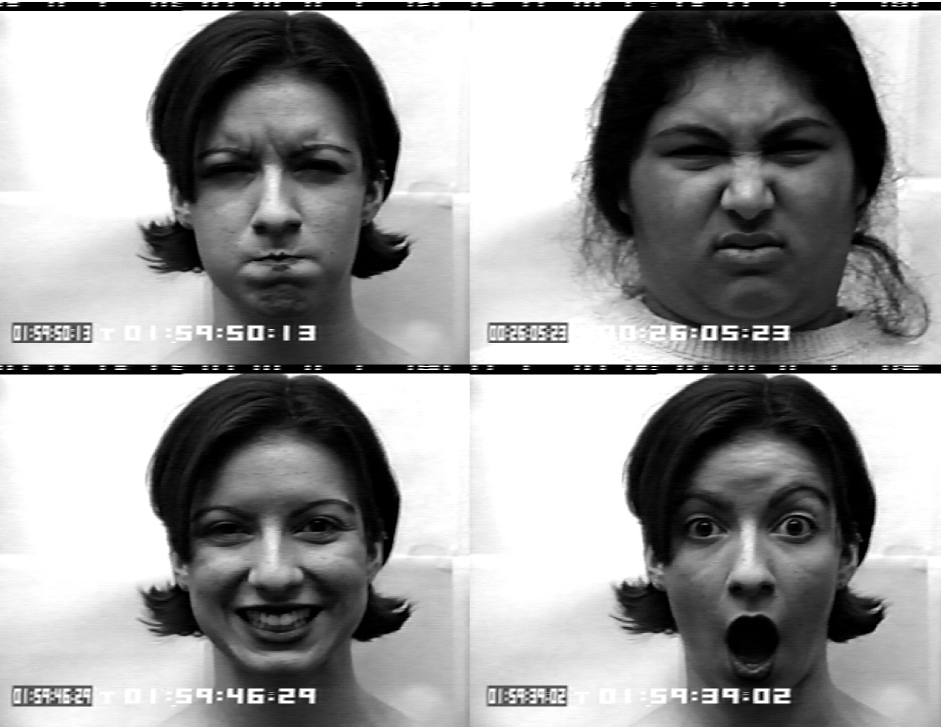
(a)

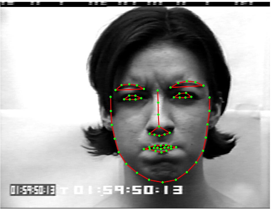
(b)

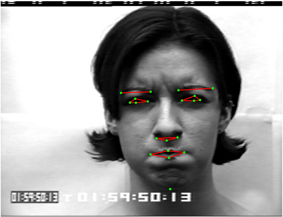
(c)

Figure 1: Cohn-Kanade emotion recognition example. a) Sample faces from CK database. b) Facial landmarks provided by CK database Lucey et al. (2010). c) Key shape points according to Valstar and Pantic (2012)

.

In this experiment, we model the coordinate $x$, and the coordinate $y$ of each landmark, as a time series, this is, $x(t)$, and $y(t)$. With $19$ landmarks, and two time series per landmark, we are modeling multivariate time series of dimension $D=38$. The length of each time series $N$ was fixed in this first experiment to 71, using a dynamic time warping algorithm for multiple signals Zhou and De la Torre Frade (2012). Our matrices $\mathbf{F}_{m}^{l}\in\mathbb{R}^{38\times 71}$. For each class, we have $L=40$ instances, and use 70% for the training set, and 30% for validation set. We repeated the experiments five times. Each time, we had different instances in the training set and the validation set. We trained multi-output GPs with FITC and PITC approximations, both fixing, and optimizing the auxiliary variables for the low rank approximations. The number of auxiliary variables was $K=25$. When not optimized, the auxiliary variables were uniformly placed along the input space.

Accuracy results are shown in Table 1. The table provides the mean, and the standard deviation for the results of the five repetitions of the experiment. The star symbol (*) on the method name means that the auxiliary input points were optimized, otherwise the auxiliary points were fixed.

Method	Generative		MCE
FITC	79.58  $\pm$	4.52	89.55  $\pm$	2.53
PITC	69.16  $\pm$	16.82	87.07  $\pm$	5.77
FITC*	79.16  $\pm$	3.29	89.16  $\pm$	6.49
PITC*	70.83  $\pm$	16.21	85.82  $\pm$	3.73
HMM (3)	85.80  $\pm$	7.26	84.15  $\pm$	9.60
HMM (5)	79.00  $\pm$	3.74	87.91  $\pm$	4.27
HMM (7)	70.80  $\pm$	8.87	91.66  $\pm$	6.08

Table 1: Classification accuracy (mean and standard deviation) for emotion recognition on the Cohn-Kanade database using dynamic time warping on the features. The asterisk in the table means that we also optimized the locations of the auxiliary variables for the low rank approximation.

Gen and Disc refer to the generative and discriminative training, using either the multi-output GP or the HMM. The table shows that for multi-output GPs, discriminative training leads to better results than the generative training. The table also shows results for HMM with 3, 5 and 7 hidden states respectively. Results for the HMM with generative training, and the multi-output GP with generative training are within the same range, if we take into account the standard deviation. Accuracies are also similar, when comparing the HMM trained with MCE, and the multi-output GP trained with MCE. We experimentally show then that the multi-output GP is as good as the HMM for emotion recognition.

3.2 Activity Recognition With Motion Capture Data Set

For the second experiment, we use a motion capture database (MOCAP) to classify between walking and running actions. In MOCAP, the input consists of the different angles between the bones of a 3D skeleton. The camera used for the MOCAP database has a frame rate of 120 frames per second, but in this experiment we sub-sampled the frames to $\frac{1}{8}$ of the original frame rate. Our motion capture data set is from the CMU motion capture data base. We considered two different categories of movement: running and walking. For running, we take subject 2 motion 3, subject 9 motions 1$-$11, subject 16 motions 35, 36, 45, 46, 55, 56, subject 35 motions 17$-$26, subject 127 motions 3, 6, 7, 8, subject 141 motions 1, 2, 3 34, subject 143 motions 1, 42, and for walking we take subject 7 motions 1$-$11, subject 8 motions 1$-$10, subject 35 motions 1$-$11, subject 39 motions 1$-$10. Figure 2 shows an example for activity recognition in MOCAP database. In this example then, we have two classes, $M=2$, and $D=62$ time courses of angles, modeled as a multi-variate time series. We also have $L_{1}=38$ for running, and $L_{2}=42$ for walking.

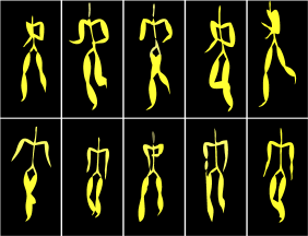
Figure 2: Sample actions from MOCAP database, run action (above) and walk action (below).

Here again we compare the generative and discriminative approaches on both our proposed model with FITC and PITC approximations and HMMs. Again, we assume $K=25$. One important difference between the experiment of section 3.1, and this experiment is that we are using the raw features here, whereas in the experiment of section 3.1, we first performed dynamic time warping to make that all the time series have the same length. It means that for this experiment, $N_{m}^{l}$ actually depends on the particular $m$, and $l$.

Method	Generative		Discriminative
FITC	60.68  $\pm$	3.98	95.71  $\pm$	2.98
PITC	76.40  $\pm$	12.38	93.56  $\pm$	5.29
FITC*	58.90  $\pm$	0.00	96.78  $\pm$	1.95
PITC*	69.28  $\pm$	15.28	84.90  $\pm$	11.33
HMM (3)	96.70  $\pm$	2.77	97.95  $\pm$	2.23
HMM (5)	94.69  $\pm$	4.36	96.32  $\pm$	0.82
HMM (7)	92.24  $\pm$	4.49	99.77  $\pm$	0.99

Table 2: Classification accuracy rates (mean and standard deviation) for activity identification on the CMU-MOCAP database.

The results are shown in Table 2 for five repeats of the experiment. For each repeat, we used $15$ instances for training, and the rest in each class, for validation. Again the results are comparable with the results of the HMM within the standard deviation. As before, the discriminative approach shows in general better results than the generative approach.

Experiments in this section and section 3.1, show that multi-output GPs exhibit similar performances to HMM, when used for pattern recognition of different types of multi-variate time series.

3.3 Subject Identification on a Motion Capture Data Set

For the third experiment we took again the CMU MOCAP database but instead of classifying between different actions, we recognized subjects by their walking styles. We considered three different subjects exhibiting walk movements. To perform the identification we took subject 7 motions 1,2,3,6,7,8,9,10, subject 8 motions 1,2,3,5,6,8,9,10, and subject 35 motions 1$-$8. Then for each subject we took four instances for training and other four repetitions for validation. Figure 3 shows an example for subject identification in the CMU-MOCAP database. We then have $M=3$, $D=62$, $L=8$, and the length for each instance, $N_{m}^{l}$, was variable.

For this experiment, we supposed the scenario where the frame rate for the motions used in training could be different from the frame rate for the motions used in testing. This configuration simulates the scenario where cameras with different recording rates are used to keep track of human activities. Notice that HMMs are not supposed to adapt well to this scenario, since the Markov assumption is that the current state depends only on the previous state. However, the Gaussian process captures the dependencies of any order, and encodes those dependencies in the kernel function, which is a continuous function of the input variables. Thus, we can evaluate the GP for any set of input points, at the testing stage, without the need to train the whole model again.

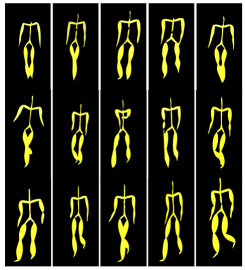
Figure 3: Sample walk actions from CMU MOCAP database, subjects 7, 8 and 35.

Table 3 shows the results of this experiment. In the table, we study three different scenarios: one for which the frame rate in the training instances was slower than in the validation instances, one for which it was faster, and one for which it was the same. We manipulate the frame rates by decimating in training (DT), and decimating in validation (DV). For example, a decimation of $\frac{1}{16}$ means that one of each 16 frames of the original time series is taken. When the validation frame rate is faster than the training frame rate (column Faster in Table 3), the performance of the multi-output GP is clearly superior to the one exhibited by the HMM, both for the generative and the discriminative approaches. When the validation frame rate is slower or equal than the training frame rate (columns Slower and Equal), we could say that the performances are similar (within the standard deviation) for multi-output GPs and HMM, if they are trained with MCE. If the models are trained generatively, the multi-output GP outperforms the HMM. Although the results for the HMM in Table 3 were obtained fixing the number of states to seven, we also performed experiments for three and five states, obtaining similar results. This experiment shows an example, where our model is clearly useful to solve a problem that a HMM does not solve satisfactorily.

Method	Faster		Slower		Equal
FITC Gen	93.28  $\pm$	3.76	94.96  $\pm$	4.60	94.96  $\pm$	4.60
PITC Gen	93.28  $\pm$	3.76	94.96  $\pm$	4.60	94.96  $\pm$	4.60
FITC MCE	94.96  $\pm$	4.60	89.96  $\pm$	9.12	89.96  $\pm$	9.12
PITC MCE	94.96  $\pm$	4.60	93.28  $\pm$	3.76	88.32  $\pm$	12.63
HMM Gen (7)	33.33  $\pm$	0.00	36.40  $\pm$	12.56	81.60  $\pm$	6.98
HMM MCE (7)	83.33  $\pm$	16.6	94.90  $\pm$	4.60	100.00  $\pm$	0.00

Table 3: Classification accuracy rates (mean and standard deviation) of subject identification by his walking style on the CMU-MOCAP database. The first column (Faster) shows the results for when the validation camera is 4 times faster than the training camera (DT = $\frac{1}{32}$, DV = $\frac{1}{8}$). The second column (Slower) shows the results for when the validation camera is 4 times slower than the training camera (DT = $\frac{1}{8}$, DV=$\frac{1}{32}$). The last column (Equal) shows the results for when both the validation and training cameras have the same frequency (DT = $\frac{1}{8}$, DV=$\frac{1}{8}$).

3.4 Face Recognition

The goal of the fourth experiment is to show an example where the vector-valued function is dependent on input variables with dimensionality greater than one, functions of multi-dimensional inputs $(f(\mathbf{x}_{0}),f(\mathbf{x}_{1}),...,f(\mathbf{x}_{n}))$ like space. The HMMs as used here are not easily generalized in this case and, thus, we do not present results with HMMs for this experiment. In this problem we work with face recognition from pictures of the Georgia Tech database . This database, contains images of 50 subjects stored in JPEG format with $640\times 480$ pixel resolution. For each individual 15 color images were taken, considering variations in illumination, facial expression, face orientations and appearance (presence of faces using glasses). Figure 4 shows an example for the Georgia Tech Face database.

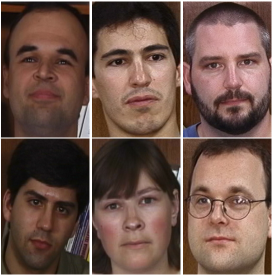
Figure 4: Sample faces from Georgia Tech Face database.

Here we did two experiments. The first experiment was carried out taking 5 subjects of the Georgia Tech database that did not have glasses. For the second experiment we took another 5 subjects of the database that had glasses. In both experiments, each image was divided in a given number of regions of equal aspect ratio. For each region $n$ we computed its centroid $\mathbf{x}_{n}$ and a texture vector $\mathbf{f}_{n}$. Notice that this can be directly modeled by a multi-output GP where the input vectors $\mathbf{x}_{n}$ are two dimensional.

Method	Gen		Disc
FITC	61.57  $\pm$	3.50	86.84  $\pm$	0.01
PITC	64.72  $\pm$	2.34	95.78  $\pm$	8.03
FITC*	66.71  $\pm$	3.82	96.84  $\pm$	7.06
PITC*	73.68  $\pm$	5.88	96.30  $\pm$	3.00

Table 4: Recognition accuracy (mean and standard deviation) for faces without glasses using a grid of size BX=4, BY=7.

Method	Gen		Disc
FITC	51.57  $\pm$	3.5	88.42  $\pm$	2.35
PITC	69.47  $\pm$	3.53	83.68  $\pm$	4.30
FITC*	56.80  $\pm$	2.44	86.84  $\pm$	0.01
PITC*	62.10  $\pm$	8.24	87.36  $\pm$	1.17

Table 5: Recognition accuracy (mean and standard deviation) for faces without glasses using a grid of size BX=6, BY=7.

Method	Gen		Disc
FITC	54.73  $\pm$	6.55	81.57  $\pm$	3.7
PITC	64.21  $\pm$	9.41	81.57  $\pm$	7.2
FITC*	60.53  $\pm$	0.02	90.52  $\pm$	9.41
PITC*	69.47  $\pm$	9.41	77.36  $\pm$	8.24

Table 6: Recognition accuracy (mean and standard deviation) for faces with glasses using a grid of BX=4, BY=7.

Method	Gen		Disc
FITC	42.1  $\pm$	0.02	93.68  $\pm$	2.35
PITC	35.78  $\pm$	2.35	86.84  $\pm$	0.01
FITC*	72.6  $\pm$	5.45	86.84  $\pm$	0.01
PITC*	48.42  $\pm$	2.35	89.47  $\pm$	0.01

Table 7: Recognition accuracy (mean and standard deviation) for faces with glasses using a grid of BX=6, BY=7.

Tables 4, 5, 6 and 7 show the results of this experiment with the discriminative and the generative training approaches. The number of divisions in the X and Y coordinates are BX and BY respectively. The features extracted from each block are mean RGB values and Segmentation-based Fractal Texture Analysis (SFTA) Costa et al. (2012) of each block. The SFTA algorithm extracts a feature vector from each region by decomposing it into a set of binary images, and then computing a scalar measure based on fractal symmetry for each of those binary images.

The results show high accuracy in the recognition process in both schemes (Faces with glasses and faces without glasses) when using discriminative training. For all the settings, the results of the discriminative training method are better than the results of the generative training method. This experiment shows the versatility of the multi-output Gaussian process to work in applications that go beyond time series classification.

4 Conclusions

In this report, we advocated the use of multi-output GPs as generative models for vector-valued random fields. We showed how to estimate the hyperparameters of the multi-output GP in a generative way and in a discriminative way, and through different experiments we demonstrated that the performance of our framework is equal or better than its natural competitor, a HMM.

For future work, we would like to study the performance of the framework using alternative discriminative criteria, like Maximum Mutual Information (MMI) using gradient optimization or Conditional Expectation Maximization Jebara (2004). We would also like to try practical applications for which there is the need to classify vector-valued functions with higher dimensionality input spaces. Computational complexity is still an issue, we would like to implement alternative efficient methods for training the multi-output GPs Hensman et al. (2013).

References

- Álvarez and Lawrence (2009) Mauricio A. Álvarez and Neil D. Lawrence. Sparse convolved Gaussian processes for multi-output regression. In Daphne Koller, Dale Schuurmans, Yoshua Bengio, and Léon Bottou, editors, NIPS, volume 21, pages 57–64, Cambridge, MA, 2009. MIT Press.
- Alvarez and Lawrence (2011) Mauricio A Alvarez and Neil D Lawrence. Computationally efficient convolved multiple output Gaussian processes. The Journal of Machine Learning Research, 12:1459–1500, 2011.
- Álvarez et al. (2012) Mauricio A. Álvarez, Lorenzo Rosasco, and Neil D. Lawrence. Kernels for vector-valued functions: a review. Foundations and Trends® in Machine Learning, 4(3):195–266, 2012.
- Bishop (2007) Christopher M. Bishop. Pattern Recognition And Machine Learning (Information Science And Statistics). Springer, 2007. URL http://www.openisbn.com/isbn/9780387310732/.
- Bonilla et al. (2008) Edwin V. Bonilla, Kian Ming Chai, and Christopher K. I. Williams. Multi-task Gaussian process prediction. In John C. Platt, Daphne Koller, Yoram Singer, and Sam Roweis, editors, NIPS, volume 20, Cambridge, MA, 2008. MIT Press.
- Boyle and Frean (2005) Phillip Boyle and Marcus Frean. Dependent Gaussian processes. In Lawrence Saul, Yair Weiss, and Léon Bouttou, editors, NIPS, volume 17, pages 217–224, Cambridge, MA, 2005. MIT Press.
- Chai (2012) Kian Ming Chai. Variational multinomial logit Gaussian process. Journal of Machine Learning Research, 13:1745–1808, 2012.
- Costa et al. (2012) A.F. Costa, G. Humpire-Mamani, and A. J M Traina. An efficient algorithm for fractal analysis of textures. In Graphics, Patterns and Images (SIBGRAPI), 2012 25th SIBGRAPI Conference on, pages 39–46, Aug 2012. doi: 10.1109/SIBGRAPI.2012.15.
- Goovaerts (1997) Pierre Goovaerts. Geostatistics For Natural Resources Evaluation. Oxford University Press, USA, 1997.
- Gopalakrishnan et al. (1991) P. Gopalakrishnan, D. Kanevsky, A. Nádas, and D. Nahamoo. An inequality for rational functions with applications to some statistical estimation problems. IEEE Transactions on Information Theory, 37:107–113, 1991.
- Hensman et al. (2013) James Hensman, Nicolò Fusi, and Neil D. Lawrence. Gaussian processes for big data. In Proceedings of UAI, 2013.
- Higdon (2002) David M. Higdon. Space and space-time modelling using process convolutions. In C. Anderson, V. Barnett, P. Chatwin, and A. El-Shaarawi, editors, Quantitative methods for current environmental issues, pages 37–56. Springer-Verlag, 2002.
- Jebara (2004) Tony Jebara. Machine Learning: Discriminative and Generative. Springer, 2004.
- Juang et al. (1997) Biing-Hwang Juang, Wu Hou, and Chin-Hui Lee. Minimum classification error rate methods for speech recognition. Speech and Audio Processing, IEEE Transactions on, 5(3):257–265, 1997.
- Lucey et al. (2010) P. Lucey, J.F. Cohn, T. Kanade, J. Saragih, Z. Ambadar, and I. Matthews. The extended cohn-kanade dataset (ck+): A complete dataset for action unit and emotion-specified expression. In Computer Vision and Pattern Recognition Workshops (CVPRW), 2010 IEEE Computer Society Conference on, pages 94–101, June 2010. doi: 10.1109/CVPRW.2010.5543262.
- Rabiner (1989) Lawrence Rabiner. A tutorial on hidden Markov models and selected applications in speech recognition. Proceedings of the IEEE, 77(2):257–286, Feb 1989. ISSN 0018-9219. doi: 10.1109/5.18626.
- Rasmussen and Williams (2006) Carl Edward Rasmussen and Christopher K. I. Williams. Gaussian Processes for Machine Learning. MIT Press, Cambridge, MA, 2006. ISBN 0-262-18253-X.
- Skolidis and Sanguinetti (2011) Grigorios Skolidis and Guido Sanguinetti. Bayesian multitask classification with Gaussian process priors. IEEE Transactions on Neural Networks, 22(12):2011 – 2021, 2011.
- Teh et al. (2005) Yee Whye Teh, Matthias Seeger, and Michael I. Jordan. Semiparametric latent factor models. In Robert G. Cowell and Zoubin Ghahramani, editors, AISTATS 10, pages 333–340, Barbados, 6-8 January 2005. Society for Artificial Intelligence and Statistics.
- Valstar and Pantic (2012) M. F. Valstar and M. Pantic. Fully automatic recognition of the temporal phases of facial actions. IEEE Transactions on Systems, Man and Cybernetics, 42:28–43, 2012.
- Zhou and De la Torre Frade (2012) Feng Zhou and Fernando De la Torre Frade. Generalized time warping for multi-modal alignment of human motion. In Proceedings of the IEEE Conference on Computer Vision and Pattern Recognition (CVPR), pages 1282–1289, June 2012.