How to include fermions into General relativity by exotic smoothness

Abstract

This paper is two-fold. At first we will discuss the generation of source terms in the Einstein-Hilbert action by using (topologically complicated) compact 3-manifolds. There is a large class of compact 3-manifolds with boundary: a torus given as the complement of a (thickened) knot admitting a hyperbolic geometry, denoted as hyperbolic knot complements in the following. We will discuss the fermionic properties of this class of 3-manifolds, i.e. we are able to identify a fermion with a hyperbolic knot complement. Secondly we will construct a large class of space-times, the exotic $\mathbb{R}^{4}$, containing this class of 3-manifolds naturally. We begin with a topological trivial space, the $\mathbb{R}^{4}$, and change only the differential structure to obtain many nontrivial 3-manifolds. It is known for a long time that exotic $\mathbb{R}^{4}$’s generate extra sources of gravity (Brans conjecture) but here we will analyze the structure of these source terms more carefully. Finally we will state that adding a hyperbolic knot complement will result in the appearance of a fermion as source term in the Einstein-Hilbert action.

Keywords: Source terms Einstein-Hilbert action, fermions as knot complements, exotic $\mathbb{R}^{4}$, adding matter by adding 3-manifolds

1 Introduction

General relativity (GR) has changed our understanding of space-time. In parallel, the appearance of quantum field theory (QFT) has modified our view of particles, fields and the measurement process. The usual approach for the unification of QFT and GR, to a theory of quantum gravity, starts with a proposal to quantize GR and its underlying structure, space-time. There is a unique opinion in the community about the relation between geometry and quantum theory: The geometry as used in GR is classical and should emerge from a quantum gravity in the limit (Planck’s constant tends to zero). Most theories went a step further and try to get a space-time from quantum theory. Then, the model of a smooth manifold is not suitable to describe quantum gravity. There is no evidence for discrete space-time structure or higher dimensions in current experiments. Therefore, we will consider a smooth 4-manifold as a model to describe the space-time in classical and quantum gravity. This view is not in conflict with quantized areas and volumes, see the example of Mostow rigidity (in subsection 3.3). But then one has the problem to represent QFT by geometric methods (submanifolds for particles or fields etc.) as well to quantize GR. Here, the exotic smoothness structure of 4-manifolds can help to find a way. A lot of work was done in the last decades to fulfill this goal. It starts with the work of Brans and Randall BR (93) and of Brans alone Bra94b ; Bra94a ; Bra (99) where the special situation in exotic 4-manifolds (in particular the exotic $\mathbb{R}^{4}$) was explained. One main result of this time was the Brans conjecture: exotic smoothness can serve as an additional source of gravity. It was confirmed for compact manifolds by Asselmeyer Ass (96) and for the exotic $\mathbb{R}^{4}$ by Sładkowski Sła (99, 01). But this conjecture was extended in AMB (02) to conjecture the generation for all forms of known energy, especially dark matter and dark energy. For dark energy we were partly successful in AMK14b where we calculated the expectation value of an embedded surface. This value showed an inflationary behavior and we were also able to calculate a cosmological constant having a realistic value (in agreement with the Planck satellite results).

The inclusion of QFT was also another goal of our approach. We showed AMK14a that an exotic 4-manifold (and therefore the space-time) has a complicated foliation. Using noncommutative geometry, we were able to study these foliations and got relations to QFT. For instance, the von Neumann algebra of a codimension-1 foliation of an exotic $\mathbb{R}^{4}$ must contain a factor of type $I\!I\!I_{1}$ used in local algebraic QFT to describe the vacuumAMK10a ; AMK11a ; AMM (12). But why is an exotic 4-manifold so complicated? As an example let us consider the exotic $S^{3}\times\mathbb{R}$. Clearly, there is always a topologically embedded 3-sphere but there is no smoothly embedded one. Let us assume the well-known hyperbolic metric of the space-time $S^{3}\times\mathbb{R}$ using the trivial foliation into leafs $S^{3}\times\left\{t\right\}$ for all $t\in\mathbb{R}$. Now we demand the exotic smoothness structure at the same time. Then we will get only topologically embedded 3-spheres, the leafs $S^{3}\times\left\{t\right\}$ (otherwise one obtains the standard smoothness structure, see CN (12) for instance). These topologically embedded 3-spheres are also known as wild 3-spheres. In AMK11b , we presented a relation to quantum D-branes. Finally we proved in AMK (13) that the deformation quantization of a tame embedding (the usual embedding) is a wild embedding. Furthermore we obtained a geometric interpretation of quantum states: wildly embedded submanifolds are quantum states. Importantly, this construction depends essentially on the continuum, wildly embedded submanifolds are always infinite triangulations. This approach opens a way to quantize a theory using geometric methods.

For a special class of compact 4-manifolds we showed in AMR (12) that exotic smoothness can generate fermions and gauge fields using the so-called knot surgery of Fintushel and Stern FS (98). Here, the knot is directly related to the appearance of an exotic smoothness structure, i.e. for two knots with different Alexander polynomials (a knot invariant) one obtains non-diffeomorphic 4-manifolds. From the physics point of view, the knot is somehow related to the fermions (and gauge fields for complicated knots). Therefore, one obtains a fixed configuration of fermions for every exotic 4-manifold (using Fintushel-Stern knot surgery) or the number of fermions is conserved. But in QFT, one is faced with the problem to have a variable number of particles. This concept cannot be realized by using a fixed configuration of fermions like in Fintushel-Stern knot surgery. Instead one needs a more flexible exotic 4-manifold with a variety of submanifolds which is related to the exotic smoothness structure. In this paper we will present an approach using the exotic $\mathbb{R}^{4}$ which will present a theory with variable particle number in difference to AMR (12).

The results of this paper are two-fold: at first we will show how to generated fermions from hyperbolic 3-manifolds and secondly we will argue that the exotic $\mathbb{R}^{4}$ contains 3-manifolds which can be interpreted as fermions. The special role of the exotic $\mathbb{R}^{4}$ is given by the fact (for all known exotic $\mathbb{R}^{4}$) that every neighborhood of a compact subset in the exotic $\mathbb{R}^{4}$ is surrounded by a compact 3-manifold (not homeomorphic to the 3-sphere) but cannot be surrounded by a (smoothly embedded) 3-sphere. Therefore we obtain always a non-trivial 3-manifold from an exotic $\mathbb{R}^{4}$ whereas for the standard $\mathbb{R}^{4}$ one can always choose a neighborhood which is surrounded by a 3-sphere. But this non-trivial 3-manifold in the exotic $\mathbb{R}^{4}$ is not uniquely determined, it depends on the representation of the exotic $\mathbb{R}^{4}$ and on the choice of the neighborhood. At this point we obtain a non-trivial 3-manifold which is not uniquely determined in contrast to AMR (12). Secondly, the Fintushel-Stern knot surgery in AMR (12) uses directly the knot complement and the Dirac action follows by a special choice of a surface (using the Weierstrass representation). In this paper we will consider directly the embedding of the 3-manifold into the 4-manifold to get the Dirac action on the 3-manifold as well as an extension to the Dirac action on the 4-manifold. Then the 3-manifold is represented by ($0-$framed) surgery along the $n$th (untwisted) Whitehead double of some knot. The choice of the level of the Whitehead double is one freedom but there is more room for ambiguities. By this method one obtains a decomposition of the 3-manifold into knot complements again (see subsection 3.3) but the representation of the 3-manifold by this knot is not unique. Therefore the decomposition of the 3-manifold can be changed by some operations (usually called Kirby calculus, see GS (99)). One can interpret this behavior in QFT where a fermion is surrounded by a ’cloud’ of virtual particles. For the exotic $\mathbb{R}^{4}$, we will obtain even this picture of non-constant particle numbers like in QFT. In our discussion above, we mixed the words fermion field, fermion and particle but we have to be more careful. We obtain the Dirac action from the embedding of the 3-manifold or the fermion field (fulfilling the Dirac equation) describes the embedding directly. But a part of this 3-manifold, the hyperbolic knot complement, has properties of a fermion, a particle of spin$\frac{1}{2}$. In the QFT picture, the excitations of the field are the particles. Then in our picture, the properties of the fermion field are given by the particular embedding and we will obtain the Dirac action for the general case. Now following the philosophy of QFT, knot complements can be seen as a kind of excitation, i.e. there are different realizations of the same 3-manifold by decompositions using knot complements. We think that only very general properties of the knot (used to get the knot complement) are connected with particle properties like charge or mass. Whereas the dynamics are related to the geometric properties of the embedding. In particular, the mean curvature of the embedding is the eigenvalue of the 3-dimensional Dirac operator (determining the 3-momentum, see equation (8) below). In our forthcoming work we will clarify this point of view more deeply.

In AMR (12) we obtained a complete picture of known matter: fermions as hyperbolic knot complements and gauge fields as torus bundles but we got only the action functionals. From the physics point of view, a fermion is a particle of spin $\frac{1}{2}$ (or $\frac{n}{2}$ in general) whose dynamics are described by the Dirac equation (or Pauli-Fierz equation in general) and they are given by the state equation $p=0$ (non-contractable matter) in the cosmological context. We will discuss all these properties in section 4 for our example of an exotic $\mathbb{R}^{4}$ but these properties will go over to the example in AMR (12). Furthermore the relation to quantum gravity has to be understand more completely. First signs of a relation can be found in Dus (10); AM (10) or by using string theory AMK10b . The results of this paper seem to suggest that an exotic $\mathbb{R}^{4}$ does not fix the concrete form of matter (fermions, gauge fields) but can fix the rules how matter can change into each other. It agrees with a philosophical interpretation of QFT where a particle is represented by a bundle of properties (Dispositional Trope Ontology, see Kuh (12)). Further work is necessary to support this conjecture.

Here is the plan of our paper. In the next section we will discuss the different constructions of exotic $\mathbb{R}^{4}$’s (large and small). But we will also describe the common property of all known examples: there is a compact subset in any known exotic $\mathbb{R}^{4}$ which cannot be surrounded by a 3-sphere. Based on this property we will also introduce the (Euclidean) Einstein-Hilbert action with boundary term. In section 3 we will describe our main method to determine the boundary term: the embedding of the 3-manifold can be described by spinors so that the boundary term of the Einstein-Hilbert action is the Dirac action for this spinor. With some effort one can extend this action from the boundary to some part of the space-time. But more importantly, the boundary can be decomposed into knot complements and we are able to interpret the knot complements admitting hyperbolic geometry as fermions in section 4. In section 5 we will discuss the Brans conjecture, i.e. the generation of source terms in General Relativity by using exotic smoothness. Our method can be also used to generate fermions by adding non-trivial 3-manifolds as shown in section 6. We will place special emphasis on spin networks and spin foams. Finally we will summarize the results. Three appendices replenish our approach with some technical details.

Finally we will state the main result of our paper: The matter content of the universe can be interpreted as being located on non-trivial 3-manifolds, which are represented by hyperbolic knot complements and graph manifolds. Then in the standard $\mathbb{R}^{4}$, we can always choose a 3-sphere to separate a compact subset from infinity or expressed in physics language, we always obtain an empty cosmos. In contrast, an exotic $\mathbb{R}^{4}$does not allow to embed a (smooth) 3-sphere separating a compact subset from infinity. But there is a non-trivial 3-manifold for separating this compact subset. Therefore, one gets a cosmos (the non-trivial 3-manifold) filled with matter. If one interprets one direction as time (for instance a radial coordinate so that the compact subset has fixed size), then matter does not exists for all times (only outside of the compact subset).

2 Construction of exotic $\mathbb{R}^{4}$

Our model of space-time is the non-compact topological $\mathbb{R}^{4}$. The results can be easily generalized for other cases such as $S^{3}\times\mathbb{R}$. In this section we will give some information about the construction of exotic $\mathbb{R}^{4}$. The existence of a smooth embedding $R^{4}\to S^{4}$ of the exotic $\mathbb{R}^{4}$ into the 4-sphere splits all exotic $\mathbb{R}^{4}$ into two classes, large (no embedding) or small. We recommend the books AMB (07) (toward physical applications of exotic smoothness), Sco (05) (for an overview of exotic manifolds) and GS (99) (for the construction of exotic 4-manifolds).

2.1 Preliminaries: Slice and non-slice knots

At first we start with some definitions from knot theory. A (smooth) knot $K$ is a smooth embedding $S^{1}\to S^{3}$. Furthermore, the $n$-disk is denoted by $D^{n}$ with $\partial D^{n}=S^{n-1}$.

Definition 1

Smoothly Slice Knot: A knot in $\partial D^{4}=S^{3}$ is smoothly slice if there exists a two-disk $D^{2}$ smoothly embedded in $D^{4}$ such that the image of $\partial D^{2}=S^{1}$ is $K$.

An example of a smoothly slice knot is the so-called Stevedore’s Knot (in Rolfsen notation $6_{1}$, see Fig. 1).

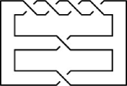
Figure 1: a smoothly slice knot: Stevedore’s knot $6_{1}$

Definition 2

Flat Topological Embedding: Let $X$ be a topological manifold of dimension $n$ and $Y$ a topological manifold of dimension $m$ where $n<m$. A topological embedding $\rho:X\to Y$ is flat if it extends to a topological embedding $\rho:X\times D^{m-n}\to Y$.

Topologically Slice Knot: A knot $K$ in $\partial D^{4}$ is topologically slice if there exists a two-disk $D^{2}$ flatly topologically embedded in $D^{4}$ such that the image of $\partial D^{2}$ is $K$.

Here we remark that the flatness condition is essential. Any knot $K\subset S^{3}$ is the boundary of a disc $D^{2}$ embedded in $D^{4}$, which can be seen by taking the cone over the knot. But the vertex of the cone is a non-flat point (the knot is crashed to a point). The difference between the smooth and the flat topological embedding is the key for the following discussion. Examples of slice knots were known for a long time. Clearly every smoothly slice knot is also a topologically slice knot but whether the reverse implication is true was not known until the work of Donaldson. But deep results from 4-manifold topology gave a negative answer: there are topologically slice knots which are not smoothly slice. An example is the pretzel knot $(-3,5,7)$ (see Fig. 2).

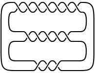
Figure 2: topological, non-smoothly slice knot: pretzel knot $(-3,5,7)$

In Fre82a , Freedman gave a topological criteria for topological sliceness: if the Alexander polynomial $\triangle_{K}(t)$ (the best known knot invariant, see Rol (76)) of the knot $K$ is trivial, $\triangle_{K}(t)=1$, then the knot $K$ is topologically slice. But the converse is wrong in general. An example how to measure the smooth sliceness is given by the smooth 4-genus $g_{4}(K)$ of the knot $K$, i.e. the minimal genus of a surface $F$ smoothly embedded in $D^{4}$ with boundary $\partial F=K$ the knot. Therefore, if the smooth 4-genus vanishes $g_{4}(K)=0$ then the knot $K$ bounds a 2-disk $D^{2}$ (surface of genus $0$) given by the smooth embedding $D^{2}\to D^{4}$ so that the image of $\partial D^{2}\to\partial D^{4}$ is the knot $K$.

2.2 Large exotic $\mathbb{R}^{4}$ and non-slice knots

Large exotic $\mathbb{R}^{4}$ can be constructed by using the failure to arbitrarily split a compact, simple-connected 4-manifold. For every topological 4-manifold one knows how to split this manifold topologically into simpler pieces using the work of Freedman Fre82b . But as shown by Donaldson Don (83), some of these 4-manifolds do not exist as smooth 4-manifolds. This contradiction between the continuous and the smooth case produces the first examples of exotic $\mathbb{R}^{4}$Gom (83). Unfortunately, the construction method is rather indirect and therefore useless for applications of the exotic $\mathbb{R}^{4}$ in physics. But as pointed out by Gompf (see Gom (85) or GS (99) Exercise 9.4.23 on p. 377ff and its solution on p. 522ff), large exotic $\mathbb{R}^{4}$ can be also constructed by using smoothly non-slice but topologically slice knots. In the following we will use the notation: $\mathbf{R^{4}}$ for the standard $\mathbb{R}^{4}$ and $R^{4}$ for the exotic $\mathbb{R}^{4}$, $\mathbb{R}^{4}$ will denote the topological structure.

Let $K$ be a knot in $\partial D^{4}$ and $X_{K}$ the two-handlebody obtained by attaching a two-handle to $D^{4}$ along $K$ with framing $0$. That means: one has a two-handle $D^{2}\times D^{2}$ which is glued to the 0-handle $D^{4}$ along its boundary using a map $f:\partial D^{2}\times D^{2}\to\partial D^{4}$ so that $f(.\,,\,x)=K\times x\subset S^{3}=\partial D^{4}$ for all $x\in D^{2}$ (or the image $im(f)=K\times D^{2}$ is the solid knotted torus). Let $\rho:X_{K}\to\mathbf{R}^{4}$ be a flat topological embedding ($K$ is topologically slice). For $K$ a smoothly non-slice knot, the open 4-manifold

$$R^{4}=\left(\mathbf{R}^{4}\setminus int\rho(X_{K})\right)\cup_{\partial X_{K}}X_{K}$$ (1)

where $int\rho(X_{K})$ is the interior of $\rho(X_{K})$, is homeomorphic but non-diffeomorphic to $\mathbf{R}^{4}$ with the standard smoothness structure (both pieces are glued along the common boundary $\partial X_{K}$). Importantly, the first term $\mathbf{R}^{4}\setminus int\rho(X_{K})$ in (1) has initially not a smooth boundary. Then the smoothing of this boundary is rather complicated (see chapter 8 in FQ (90) or Theorem 9.4.22 of GS (99)).

The proof of this fact ($R^{4}$ is exotic) is given by contradiction, i.e. let us assume $R^{4}$ is diffeomorphic to $\mathbf{R}^{4}$. Thus, there exists a diffeomorphism $R^{4}\to\mathbf{R}^{4}$. The restriction of this diffeomorphism to $X_{K}$ is a smooth embedding $X_{K}\hookrightarrow\mathbf{R}^{4}$. However, such a smooth embedding exists if and only if $K$ is smoothly slice (see GS (99)). But, by hypothesis, $K$ is not smoothly slice. Thus by contradiction, there exists no diffeomorphism $R^{4}\to\mathbf{R}^{4}$ and $R^{4}$ is exotic, homeomorphic but not diffeomorphic to $\mathbf{R}^{4}$. Finally, we have to prove that $R^{4}$ is large. $X_{K}$, by construction, is compact and a smooth submanifold of $R^{4}$. By hypothesis, $K$ is not smoothly slice and therefore $X_{K}$ can not smoothly embed in $\mathbf{R}^{4}$. Or, $R^{4}$ is a large exotic $\mathbb{R}^{4}$.

2.3 Small exotic $\mathbb{R}^{4}$ and Casson handles

Small exotic $\mathbb{R}^{4}$’s are again the result of anomalous smoothness in 4-dimensional topology but of a different kind than for large exotic $\mathbb{R}^{4}$’s. In 4-manifold topology Fre82b , a homotopy-equivalence between two compact, closed, simply-connected 4-manifolds implies a homeomorphism between them (a so-called h-cobordism). But Donaldson Don (87) provided the first smooth counterexample, i.e. both manifolds are generally not diffeomorphic to each other. The failure can be localized in some contractible submanifold (Akbulut cork) so that an open neighborhood of this submanifold is a small exotic $\mathbb{R}^{4}$. The whole procedure implies that this exotic $\mathbb{R}^{4}$ can be embedded in the 4-sphere $S^{4}$.

The idea of the construction is simply given by the fact that every such smooth h-cobordism between non-diffeomorphic 4-manifolds can be written as a product cobordism except for a compact contractible sub-h-cobordism $V$, the Akbulut cork. An open subset $U\subset V$ homeomorphic to $[0,1]\times{{\mathbb{R}}^{4}}$ is the corresponding sub-h-cobordism between two exotic ${{\mathbb{R}}^{4}}$’s. These exotic ${{\mathbb{R}}^{4}}$’s are called ribbon ${{\mathbb{R}}^{4}}$’s. They have the important property of being diffeomorphic to open subsets of the standard ${{\mathbb{R}}^{4}}$. To be more precise, consider a pair $(X_{+},X_{-})$ of homeomorphic, smooth, closed, simply-connected 4-manifolds.

Theorem 2.1

(GS (99) Theorem 9.3.1) Let $W$ be a smooth h-cobordism between closed, simply connected 4-manifolds $X_{-}$ and $X_{+}$. Then there is an open subset $U\subset W$ homeomorphic to $[0,1]\times{{\mathbb{R}}^{4}}$ with a compact subset $C\subset U$ such that the pair $(W\setminus C,U\setminus C)$ is diffeomorphic to a product $[0,1]\times(X_{-}\setminus C,U\cap X_{-}\setminus C)$. The subsets $R_{\pm}=U\cap X_{\pm}$ (homeomorphic to ${{\mathbb{R}}^{4}}$) are diffeomorphic to open subsets of ${{\mathbb{R}}^{4}}$. If $X_{-}$ and $X_{+}$ are not diffeomorphic, then there is no smooth 4-ball in $R_{\pm}$ containing the compact set $Y_{\pm}=C\cap R_{\pm}$, so both $R_{\pm}$ are exotic ${{\mathbb{R}}^{4}}$’s.

Thus, $R_{-}$ lies in a compact set, i.e. a 4-sphere or $R_{-}$ is a small exotic $\mathbb{R}^{4}$. In DF (92) Freedman and DeMichelis constructed also a continuous family of small exotic $\mathbb{R}^{4}$. Now we are ready to discuss the decomposition of a small exotic $\mathbb{R}^{4}$ by Bizaca and Gompf BG (96) by using special pieces, the handles forming a handle body. Every 4-manifold can be decomposed (seen as handle body) using standard pieces such as $D^{k}\times D^{4-k}$, the so-called $k$-handle attached along $\partial D^{k}\times D^{4-k}$ to the boundary $S^{3}=\partial D^{4}$ of a $0-$handle $D^{0}\times D^{4}=D^{4}$. The construction of the handle body can be divided into two parts. The first part is the manifold $Y_{-}$ in the theorem above, whereas the second part is the Casson handle $CH$ which will be considered now.

Let us start with the basic construction of the Casson handle $CH$. Let $M$ be a smooth, compact, simple-connected 4-manifold and $f:D^{2}\to M$ a (codimension-2) mapping. By using diffeomorphisms of $D^{2}$ and $M$, one can deform the mapping $f$ to get an immersion (i.e. injective differential) generically with only double points (i.e. $\#|f^{-1}(f(x))|=2$) as singularities GG (73). But to incorporate the generic location of the disk, one is rather interested in the mapping of a 2-handle $D^{2}\times D^{2}$ induced by $f\times id:D^{2}\times D^{2}\to M$ from $f$. Then every double point (or self-intersection) of $f(D^{2})$ leads to self-plumbings of the 2-handle $D^{2}\times D^{2}$. A self-plumbing is an identification of $D_{0}^{2}\times D^{2}$ with $D_{1}^{2}\times D^{2}$ where $D_{0}^{2},D_{1}^{2}\subset D^{2}$ are disjoint sub-disks of the first factor disk. Consider the pair $(D^{2}\times D^{2},\partial D^{2}\times D^{2})$ and produce finitely many self-plumbings away from the attaching region $\partial D^{2}\times D^{2}$ to get a kinky handle $(k,\partial^{-}k)$ where $\partial^{-}k$ denotes the attaching region of the kinky handle. A kinky handle $(k,\partial^{-}k)$ is a one-stage tower $(T_{1},\partial^{-}T_{1})$ and an $(n+1)$-stage tower $(T_{n+1},\partial^{-}T_{n+1})$ is an $n$-stage tower union of kinky handles $\bigcup_{\ell=1}^{n}(T_{\ell},\partial^{-}T_{\ell})$ where two towers are attached along $\partial^{-}T_{\ell}$. Let $T_{n}^{-}$ be $(\mbox{int}T_{n})\cup\partial^{-}T_{n}$ and the Casson handle

$$CH=\bigcup_{\ell=0}T_{\ell}^{-}$$

is the union of towers (with direct limit topology induced from the inclusions $T_{n}\hookrightarrow T_{n+1}$).

The main idea of the construction above is very simple: an immersed disk $D_{1}$ (disk with self-intersections) can be deformed into an embedded disk $D_{\infty}$ (disk without self-intersections) by sliding one part of the immersed disk $D_{1}$ along another disks $D_{2}$ to kill the self-intersections (one disk for every self-intersection). Unfortunately the disks $D_{2}$ can be immersed only. But the immersion can be deformed to an embedding by disks $D_{3}$ etc. In the limit of this process one ”shifts the self-intersections into infinity” and obtains the standard open 2-handle $(D_{\infty}^{2}\times\mathbb{R}^{2},\partial D_{\infty}^{2}\times\mathbb{R}^{2})$.

A Casson handle is specified up to (orientation preserving) diffeomorphism (of pairs) by a labeled finitely-branching tree with base-point *, having all edge paths infinitely extendable away from *. Each edge should be given a label $+$ or $-$ whereas each vertex corresponds to a kinky handle. The self-plumbing number of that kinky handle equals the number of branches leaving the vertex. The sign on each branch corresponds to the sign of the associated self plumbing. The whole process generates a tree with infinite many levels. In principle, every tree with a finite number of branches per level realizes a corresponding Casson handle. Each building block of a Casson handle, the “kinky” handle with $n$ kinks, is diffeomorphic to the $n-$times boundary-connected sum $\natural_{n}(S^{1}\times D^{3})$ (see appendix A) with two attaching regions. Technically speaking, one region is a tubular neighborhood of band sums of Whitehead links connected with the previous block. The other region is a disjoint union of the standard open subsets $S^{1}\times D^{2}$ in $\#_{n}S^{1}\times S^{2}=\partial(\natural_{n}S^{1}\times D^{3})$ (this is connected with the next block).

2.4 3-manifolds and exotic $\mathbb{R}^{4}$

We described the construction of large and small exotic $\mathbb{R}^{4}$’s above. Apart from the different constructions, there are some common properties of exotic $\mathbb{R}^{4}$’s which will be discussed now. Usually there are arbitrary splittings of the $\mathbb{R}^{4}$ into $\mathbb{R}^{3}\times\mathbb{R}$ or $\mathbb{R}\times\mathbb{R}\times\mathbb{R}\times\mathbb{R}$. But every manifold of dimension smaller than 4 has a unique smoothness structure. Therefore $\mathbb{R}^{3}\times\left\{t\right\}$ has a unique smoothness structure for every $t\in\mathbb{R}$ and also the whole $\mathbb{R}^{3}\times\mathbb{R}$. A standard smoothness structure on $\mathbb{R}^{4}$ is uniquely characterized by the fact that the smoothness structure respects the decomposition $\mathbb{R}^{3}\times\mathbb{R}^{1}$. But more is true: also every splitting $\Sigma\times\mathbb{R}$ using a contractable 3-manifold $\Sigma$ is diffeomorphic to $\mathbf{R}^{4}$ (standard $\mathbb{R}^{4}$), see CN (12). Expressed in physical terms: there is no globally hyperbolic metric on any exotic $\mathbb{R}^{4}$. But by using foliation theory, every exotic $\mathbb{R}^{4}$ admits a codimension-1 foliation (or there is a non-vanishing vector field which can be used to define a Lorentz metric, see Ste (99)). Therefore there must be a connection between exotic $\mathbb{R}^{4}$ and (non-trivial) codimension-1 foliations.

Another characterizing property of all known exotic $\mathbb{R}^{4}$ is the existence of a compact subset $Q\subset R^{4}$ which cannot be surrounded by a smoothly embedded 3-sphere. To express it differently, the exotic $\mathbb{R}^{4}$ does not contain 3-spheres surrounding $Q$. This fact will be the central point in our argumentation because it allows to consider non-trivial 3-manifolds (i.e. not homeomorphic to the 3-sphere). For us, it is enough to obtain a representative (i.e. a 3-manifold) for an exotic $\mathbb{R}^{4}$. We are not interested in the construction of a unique 3-manifold (characterizing the smoothness structure). Instead we will show that exotic smoothness is the source of non-trivial 3-manifolds $\Sigma$ which are embedded. In contrast, for any compact subset $Q$ of the standard $\mathbb{R}^{4}$ there is always a smoothly embedded 3-sphere surrounding $Q$. Of course the 3-manifold $\Sigma$ can be also embedded in the standard $\mathbb{R}^{4}$ (at least in case of the small exotic $\mathbb{R}^{4}$) but we will state that the exotic $\mathbb{R}^{4}$ does not contain 3-spheres surrounding $Q$ (for all known examples of exotic $\mathbb{R}^{4}$). Furthermore, the 3-manifold $\Sigma$ surrounding the compact subset $Q$ in the exotic $\mathbb{R}^{4}$ separates $Q$ from infinity. In the following we will denote the 3-manifold surrounding $Q$ by $\Sigma$. Much of the following material can be found in the section 9.4 of the book GS (99) as well in the paper Gan (06).

2.4.1 Large Exotic $\mathbb{R}^{4}$

There are only implicit examples of large exotic $\mathbb{R}^{4}$’s and our construction (1) is in principle not very useful. Let $R^{4}$ be a large exotic $\mathbb{R}^{4}$ and $Q\subset R^{4}$ a compact subset of codimension $0$. In Gan (06), a large exotic $\mathbb{R}^{4}$ called $R_{1}$ was constructed (using the co-called K3-surface) so that any possible $Q$ is surrounded by a 3-manifold $\Sigma$ with first Betti number $b_{1}$ at least $b_{1}=3$ in contrast to the 3-sphere with $b_{1}=0$.

2.4.2 Small Exotic $\mathbb{R}^{4}$

In case of a small exotic $\mathbb{R}^{4}$, there are some explicit constructions, see BG (96). Therefore, it is not surprising that there is an explicit construction (or one possible representative) for the 3-manifold $\Sigma$ surrounding a possible compact subset $Q$. It is a 3-manifold with $b_{1}=1$ ($0-$framed surgery along the $(-3,3,-3)$ pretzel knot, see Fig. 3, in the simplest case or the $n-$fold untwisted Whitehead double of it). We will fix this 3-manifold $\Sigma$ in the following.

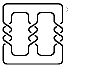
Figure 3: $(-3,3,-3)$ pretzel knot or knot $9_{46}$ (Rolfson notation)

2.5 The Einstein-Hilbert action

In this section we will discuss the (Euclidean) Einstein-Hilbert action functional

$$S_{EH}(M)=\intop_{M}R\sqrt{g}\>d^{4}x$$ (2)

of the 4-manifold $M$ and fix the Ricci-flat metric $g$ as solution of the vacuum field equations of the exotic 4-manifold. If $M$ is an exotic $\mathbb{R}^{4}$ we have to comment about the existence of a metric $g$. At first, there is a result of Taylor Tay (05) that all known exotic $\mathbb{R}^{4}$’s admit no proper Lipschitz functions having bounded critical values. This property is very restrictive but does not forbid to introduce a smooth metric $g$ (at least locally). Furthermore, it confirmed implicitly a result of us AMK14b that a cosmological model based on an exotic $\mathbb{R}^{4}$ (or better on its exotic end $S^{3}\times\mathbb{R}$) showed an inflationary behavior, i.e. with no bounded curvature etc.

In the following we will argue to obtain an additional contribution to the action functional coming from exotic smoothness. This contribution uses the property of all known exotic $\mathbb{R}^{4}$ (see the previous subsection above), i.e. the existence of a non-trivial compact 3-manifold separating a compact submanifold from infinity. Now consider a compact 4-dimensional submanifold $Q\subset R^{4}$ of an exotic $\mathbb{R}^{4}$ (large or small). Then $Q$ is surrounded by a 3-manifold $\Sigma$ which is not diffeomorphic to the 3-sphere $S^{3}$.This 3-manifold $\Sigma$ divides the exotic $\mathbb{R}^{4}$ into two parts

$$R^{4}=\overline{U}(Q)\cup_{\partial\overline{U}(Q)=\Sigma}\left(R^{4}\setminus\overline{U}(Q)\right)$$ (3)

where $\overline{U}(Q)$ is a closed neighborhood of $Q$ with boundary $\Sigma=\partial\overline{U}(Q)$. For the parts of the decomposition we obtain the action functionals

$$S_{EH}(R^{4}\setminus\overline{U}(Q)) = \intop_{R^{4}\setminus\overline{U}(Q)}R\sqrt{g}\,d^{4}x+\intop_{\partial\overline{U}(Q)}H\sqrt{h}d^{3}x$$

$$S_{EH}(\overline{U}(Q)) = \intop_{\overline{U}(Q)}R\sqrt{g}d^{4}x-\intop_{\partial\overline{U}(Q)}H\sqrt{h}d^{3}x$$

including the contribution of the boundary $\partial\overline{U}(Q)=\Sigma$ with respect to different orientations and $H$ is the trace of the second fundamental form (mean curvature) of the boundary in the metric $g$ (see AES (08); AS (08) for the discussion of the boundary terms). Interestingly, this decomposition is independent of the class, large or small, of the exotic $\mathbb{R}^{4}$. In the following we will discuss the boundary term, i.e. we can reduce the problem to the discussion of the action

$$S_{EH}(\Sigma)=\intop_{\Sigma}H\,\sqrt{h}\,d^{3}x$$ (4)

along the boundary $\Sigma$ (a 3-manifold). It is a surprise that this integral agrees with the Dirac action of a spinor describing the (embedded) boundary, see below.

3 Dirac action and 3-manifolds

In the following we will show that the action (4) over a 3-manifold $\Sigma$ is equivalent to the the Dirac action of a spinor over $\Sigma$. At first we will consider the general case of an embedding of a 3-manifold into a 4-manifold. Let $\iota:\Sigma\hookrightarrow M$ be an embedding of the 3-manifold $\Sigma$ into the 4-manifold $M$ with the normal vector $\vec{N}$. A small neighborhood $U_{\epsilon}$ of $\iota(\Sigma)\subset M$ looks like $U_{\epsilon}=\iota(\Sigma)\times[0,\epsilon]$. Furthermore we identify $\Sigma$ and $\iota(\Sigma)$ ($\iota$ is an embedding). Every 3-manifold admits a spin structure with a spin bundle, i.e. a principal $Spin(3)=SU(2)$ bundle (spin bundle) as a lift of the frame bundle (principal $SO(3)$ bundle associated to the tangent bundle). There is a (complex) vector bundle associated to the spin bundle (by a representation of the spin group), called spinor bundle $S_{\Sigma}$. A section in the spinor bundle is called a spinor field (or a spinor). In case of a 4-manifold, we have to assume the existence of a spin structure. But for a manifold like $\mathbb{R}^{4}$, there is no restriction, i.e. there is always a spin structure and a spinor bundle $S_{M}$. In general, the unitary representation of the spin group in $D$ dimensions is $2^{[D/2]}$-dimensional. From the representational point of view, a spinor in 4 dimensions is a pair of spinors in dimension 3. Therefore, the spinor bundle $S_{M}$ of the 4-manifold splits into two sub-bundles $S_{M}^{\pm}$ where one subbundle, say $S_{M}^{+},$ can be related to the spinor bundle $S_{\Sigma}$ of the 3-manifold. Then the spinor bundles are related by $S_{\Sigma}=\iota^{*}S_{M}^{+}$ with the same relation $\phi=\iota_{*}\Phi$ for the spinors ($\phi\in\Gamma(S_{\Sigma})$ and $\Phi\in\Gamma(S_{M}^{+})$). Let $\nabla_{X}^{M},\nabla_{X}^{\Sigma}$ be the covariant derivatives in the spinor bundles along a vector field $X$ as section of the bundle $T\Sigma$. Then we have the formula

$$\nabla_{X}^{M}(\Phi)=\nabla_{X}^{\Sigma}\phi-\frac{1}{2}(\nabla_{X}\vec{N})\cdot\vec{N}\cdot\phi$$ (5)

with the obvious embedding $\phi\mapsto\left(\begin{array}[]{c}\phi\\ 0\end{array}\right)=\Phi$ of the spinor spaces from the relation $\phi=\iota_{*}\Phi$. The expression $\nabla_{X}\vec{N}$ is the second fundamental form of the embedding where the trace $tr(\nabla_{X}\vec{N})=2H$ is related to the mean curvature $H$. Then from (5) one obtains the following relation between the corresponding Dirac operators

$$D^{M}\Phi=D^{\Sigma}\phi-H\phi$$ (6)

with the Dirac operator $D^{\Sigma}$ on the 3-manifold $\Sigma$. This relation (as well as (5)) is only true for the small neighborhood $U_{\epsilon}$ where the normal vector points is parallel to the vector defined by the coordinates of the interval $[0,\epsilon]$ in $U_{\epsilon}$. In AMR (12), we extend the spinor representation of an immersed surface into the 3-space to the immersion of a 3-manifold into a 4-manifold according to the work in Fri (98). Then the spinor $\phi$ defines directly the embedding (via an integral representation) of the 3-manifold. Then the restricted spinor $\Phi|_{\Sigma}=\phi$ is parallel transported along the normal vector and $\Phi$ is constant along the normal direction (reflecting the product structure of $U_{\epsilon}$). But then the spinor $\Phi$ has to fulfill

$$D^{M}\Phi=0$$ (7)

in $U_{\epsilon}$ i.e. $\Phi$ is a parallel spinor. Finally we get

$$D^{\Sigma}\phi=H\phi$$ (8)

with the extra condition $|\phi|^{2}=const.$ (see Fri (98) for the explicit construction of the spinor with $|\phi|^{2}=const.$ from the restriction of $\Phi$). Then we can express the action (4) by using (8) to obtain

$$\intop_{\Sigma}H\,\sqrt{h}\,d^{3}x=\intop_{\Sigma}\bar{\phi}\,D^{\Sigma}\phi\,\sqrt{h}d^{3}x$$ (9)

using $|\phi|^{2}=const.$

3.1 Deformation of the Embedding as seen by the Dirac operator

Now we will discuss the deformation of an embedding using a diffeomorphism. Let $I:\Sigma\hookrightarrow M$ be an embedding of $\Sigma$ (3-manifold) into $M$ (4-manifold). A deformation of an embedding $I^{\prime}:\Sigma^{\prime}\hookrightarrow M^{\prime}$ are diffeomorphisms $f:M\to M^{\prime}$ and $g:\Sigma\to\Sigma^{\prime}$ of $M$ and $\Sigma$, respectively, so that

$$I\circ f=g\circ I^{\prime}\,.$$

One of the diffeomorphism (say $f$) can be absorbed into the definition of the embedding and we are left with one diffeomorphism $g\in Diff(\Sigma)$ to define the deformation of the embedding $I$. But as stated above, the embedding is directly related to the spinor $\phi$ on $\Sigma$ fulfilling the Dirac equation. Therefore we have to discuss the action of the diffeomorphism group $Diff(\Sigma)$ on the Hilbert space of $L^{2}-$spinors fulfilling the Dirac equation. This case was considered in the literature DD (13). The spinor space $S_{g,\sigma}(\Sigma)$ on $\Sigma$ depends on two ingredients: a (Riemannian) metric $g$ and a spin structure $\sigma$ (labeled by the number of elements in $H^{1}(\Sigma,\mathbb{Z}_{2})$). Let us consider the group of orientation-preserving diffeomorphism $Diff^{+}(\Sigma)$ acting on $g$ (by pullback $f^{*}g$) and on $\sigma$ (by a suitable defined pullback $f^{*}\sigma$). The Hilbert space of $L^{2}-$spinors of $S_{g,\sigma}(\Sigma)$ is denoted by $H_{g,\sigma}$. Then according to DD (13), any $f\in Diff^{+}(\Sigma)$ leads in exactly two ways to a unitary operator $U$ from $H_{g,\sigma}$ to $H_{f^{*}g,f^{*}\sigma}$. The (canonically) defined Dirac operator is equivariant with respect to the action of $U$ and the spectrum is invariant under (orientation-preserving) diffeomorphisms. But by the discussion above, we also do not change the embedding by a diffeomorphism. So, our whole approach is independent of a particular coordinate system i.e. $\Phi$ is a parallel spinor. In AMR (12), we used an one-parameter family of surface embeddings instead of a 3-manifold embedding. But the result remains the same: the 4-dimensional spinor $\Phi$ is a parallel spinor.

3.2 The extension to the 4-dimensional Dirac action

Above we obtained a relation (6) between a 3-dimensional spinor $\phi$ on the 3-manifold $\Sigma$ fulfilling a Dirac equation $D^{\Sigma}\phi=H\phi$ (determined by the embedding $\Sigma\to M$ into a 4-manifold $M$) and a 4-dimensional spinor $\Phi$ on a 4-manifold $M$ with fixed chirality ($\in\Gamma(S_{M}^{+})$ or $\in\Gamma(S_{M}^{-})$) fulfilling the Dirac equation $D^{M}\Phi=0$. At first we consider the variation

$$\delta\intop_{\Sigma}\bar{\phi}D^{\Sigma}\phi\>\sqrt{g}\,d^{3}x=0$$ (10)

of the 3-dimensional action leading to the Dirac equations

$$D^{\Sigma}\phi=0\quad D^{\Sigma}\bar{\phi}=0$$ (11)

or to

$$H=0\,,$$

a characterization of the embedding $\Sigma\to M$ with minimal mean curvature. This variation can be understood as a variation of the embedding. In contrast, the extension of the spinor $\phi$ (as solution of (11)) to the 4-dimensional spinor $\Phi$ by using the embedding

$$\Phi=\left(\begin{array}[]{c}\phi\\ 0\end{array}\right)$$ (12)

can be only seen as embedding, if (and only if) the 4-dimensional Dirac equation

$$D^{M}\Phi=0$$ (13)

on $M$ is fulfilled (using relation (6)). This Dirac equation is obtained by varying the action

$$\delta\intop_{M}\bar{\Phi}D^{M}\Phi\sqrt{g}\>d^{4}x=0$$ (14)

Importantly, this variation has a different interpretation in contrast to varying the 3-dimensional action. Both variations look very similar. But in (14) we vary over smooth maps $\Sigma\to M$ which are not embeddings (i.e. represented by spinors $\Phi$ with $D^{M}\Phi\not=0$). Only the choice of the extremal action selects the embedding among other smooth maps. In particular the spinor $\Phi$ (as solution of the 4-dimensional Dirac equation) is localized at the embedded 3-manifold $\Sigma$ (with respect to the embedding (12)). The 3-manifold $\Sigma$ moves along the normal vector (see the relation (5) between the covariant derivatives representing a parallel transport).

3.3 Fermions as knot complements

In the previous subsections we presented a formalism to describe the embedding of a 3-manifold into a 4-manifold by using a spinor. But one may ask whether the spinor is really connected with a field of spin $\frac{1}{2}$. To answer this question we have to analyze the structure of 3-manifolds. In short, every 3-manifold is the sum of prime 3-manifolds where a subclass (irreducible 3-manifolds) splits into hyperbolic and graph manifolds.

A connected 3-manifold $\Sigma$ is prime if it cannot be obtained as a connected sum of two manifolds $\Sigma_{1}\#\Sigma_{2}$ (see the appendix A for the definition) neither of which is the 3-sphere $S^{3}$ (or, equivalently, neither of which is the homeomorphic to $\Sigma$). Examples are the 3-torus $T^{3}$ and $S^{1}\times S^{2}$ but also the Poincare sphere. According to Mil (62), any compact, oriented 3-manifold is the connected sum of an unique (up to homeomorphism) collection of prime 3-manifolds (prime decomposition). A subset of prime manifolds are the irreducible 3-manifolds. A connected 3-manifold is irreducible if every differentiable submanifold $S$ homeomorphic to a sphere $S^{2}$ bounds a subset $D$ (i.e. $\partial D=S$) which is homeomorphic to the closed ball $D^{3}$. The only prime but reducible 3-manifold is $S^{1}\times S^{2}$. For the geometric properties (to meet Thurstons geometrization theorem) we need a finer decomposition induced by incompressible tori. A properly embedded connected surface $S\subset\Sigma$ is called 2-sided if its normal bundle is trivial, and 1-sided if its normal bundle is nontrivial. A 2-sided connected surface $S$ other than $S^{2}$ or $D^{2}$ is called incompressible if for each disk $D\subset\Sigma$ with $D\cap S=\partial D$ there is a disk $D^{\prime}\subset S$ with $\partial D^{\prime}=\partial D$. The boundary of a 3-manifold is an incompressible surface. Most importantly, the 3-sphere $S^{3}$, $S^{2}\times S^{1}$ and the 3-manifolds $S^{3}/\Gamma$ with $\Gamma\subset SO(4)$ a finite subgroup do not contain incompressible surfaces. The class of 3-manifolds $S^{3}/\Gamma$ (the spherical 3-manifolds) includes cases like the Poincare sphere ($\Gamma=I^{*}$ the binary icosaeder group) or lens spaces ($\Gamma=\mathbb{Z}_{p}$ the cyclic group). Let $K_{i}$ be irreducible 3-manifolds containing incompressible surfaces then we can $N$ split into pieces (along embedded $S^{2}$)

$$\Sigma=K_{1}\#\cdots\#K_{n_{1}}\#_{n_{2}}S^{1}\times S^{2}\#_{n_{3}}S^{3}/\Gamma\,,$$ (15)

where $\#_{n}$ denotes the $n$-fold connected sum and $\Gamma\subset SO(4)$ is a finite subgroup. The decomposition of $N$ is unique up to the order of the factors. The irreducible 3-manifolds $K_{1},\ldots,\,K_{n_{1}}$ are able to contain incompressible tori and one can split $K_{i}$ along the tori into simpler pieces $K=H\cup_{T^{2}}G$ JS (79) (called the JSJ decomposition). The two classes $G$ and $H$ are the graph manifold $G$ and hyperbolic 3-manifold $H$ (see Fig. 4).

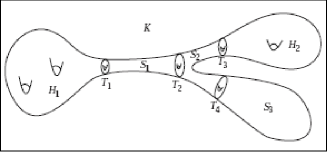
Figure 4: Torus (JSJ-) decomposition, $H_{i}$ hyperbolic manifold, $S_{i}$ Graph-manifold, $T_{i}$ Tori

The hyperbolic 3-manifold $H$ has a torus boundary $T^{2}=\partial H$, i.e. $H$ admits a hyperbolic structure in the interior only. One property of hyperbolic 3-manifolds is central: Mostow rigidity. As shown by Mostow Mos (68), every hyperbolic $n-$manifold $n>2$ with finite volume has this property: Every diffeomorphism (especially every conformal transformation) of a hyperbolic $n-$manifold with finite volume is induced by an isometry. Therefore one cannot scale a hyperbolic 3-manifold and the volume is a topological invariant. Together with the prime and JSJ decomposition

$$\Sigma=\left(H_{1}\cup_{T^{2}}G_{1}\right)\#\cdots\#\left(H_{n_{1}}\cup_{T^{2}}G_{n_{1}}\right)\#_{n_{2}}S^{1}\times S^{2}\#_{n_{3}}S^{3}/\Gamma\,,$$ (16)

we can discuss the geometric properties central to Thurstons geometrization theorem (as proved by Perelman): Every oriented closed irreducible 3-manifold can be cut along tori (JSJ decomposition), so that the interior of each of the resulting manifolds has a geometric structure with finite volume. Now, we have to introduce the term ’geometric structure’. A model geometry is a simply connected smooth manifold $X$ together with a transitive action of a Lie group $G$ on $X$ with compact stabilizers. A geometric structure on a manifold $\Sigma$ is a diffeomorphism from $\Sigma$ to $X/{\Gamma}$ for some model geometry $X$, where $\Gamma$ is a discrete subgroup of $G$ acting freely on $X$. It is a surprising fact that there are also a finite number of three-dimensional model geometries, i.e. 8 geometries with the following models: spherical $(S^{3},O_{4}(\mathbb{R}))$, Euclidean $(\mathbb{E}^{3},O_{3}(\mathbb{R})\ltimes\mathbb{R}^{3})$, hyperbolic $(\mathbb{H}^{3},O_{1,3}(\mathbb{R})^{+})$, mixed spherical-Euclidean $(S^{2}\times\mathbb{R},O_{3}(\mathbb{R})\times\mathbb{R}\times\mathbb{Z}_{2})$, mixed hyperbolic-Euclidean $(\mathbb{H}^{2}\times\mathbb{R},O_{1,3}(\mathbb{R})^{+}\times\mathbb{R}\times\mathbb{Z}_{2})$ and 3 exceptional cases called $\tilde{SL}_{2}$ (twisted version of $\mathbb{H}^{2}\times\mathbb{R}$), NIL (geometry of the Heisenberg group as twisted version of $\mathbb{E}^{3}$), SOL (split extension of $\mathbb{R}^{2}$ by $\mathbb{R}$, i.e. the Lie algebra of the group of isometries of the 2-dimensional Minkowski space). We refer to Sco (83) for the details.

There are three main parts in the possible decomposition of a 3-manifold: $S^{1}\times S^{2}$, $S^{3}/\Gamma$ and $H_{i}\cup_{T^{2}}G$. We will introduce the physical property spin in the next section. In this paper we are interested in fermions with spin $\frac{1}{2}$. Using the definition of spin $\frac{1}{2}$ in the next section, the two manifolds $S^{1}\times S^{2}$ and $S^{3}/\Gamma$ have a spin different from $\frac{1}{2}$. Therefore for the moment, the two manifolds $S^{1}\times S^{2}$ and $S^{3}/\Gamma$ can be ruled out. We will discuss the case of higher spins in the next section. Then we are left with $H_{i}\cup_{T^{2}}G_{i}$. In case of a small exotic $\mathbb{R}^{4}$, we have an explicit expression of the 3-manifold $\Sigma$: it is the $0-$framed surgery along $n$th untwisted Whitehead double of the pretzel knot $(-3,3-3)$ (also known as $9_{46}$ knot in Rolfson notation, see Rol (76)). To see it explicitly, we fix $n=1$ and consider the $0-$framed surgery along the untwisted Whitehead double $K_{Wh,9_{46}}$ of the $(-3,3-3)$ pretzel knot to get a 3-manifold $\Sigma$. By definition, $\Sigma$ is decomposed like

$$\Sigma=\left(S^{3}\setminus(K_{Wh,9_{46}}\times D^{2})\right)\cup_{T^{2}}(D^{2}\times S^{1})$$ (17)

with the identity map as gluing map ($D^{2}\times S^{1}$ is a graph manifold). The 3-manifold $S^{3}\setminus(K_{Wh,9_{46}}\times D^{2})$ is the complement of the Whitehead double $K_{Wh,9_{46}}$. According to Bud (06), one can decompose this knot complement according to the JSJ-decomposition into

$$S^{3}\setminus(K_{Wh,9_{46}}\times D^{2})=\left(S^{3}\setminus(Wh\times D^{2})\right)\cup_{T^{2}}\left(S^{3}\setminus(K_{9_{46}}\times D^{2})\right)$$ (18)

i.e. in the complement of the Whitehead link $Wh$ connected to the complement of the pretzel knot $K_{9_{46}}$. It is known that both complements are hyperbolic 3-manifolds. Finally we see that $\Sigma$ can be decomposed into $\Sigma=H_{1}\cup_{T^{2}}H_{2}\cup_{T^{2}}G$ with $H_{1}=S^{3}\setminus(K_{9_{46}}\times D^{2})$, $H_{2}=S^{3}\setminus(Wh\times D^{2})$ and $G=D^{2}\times S^{1}$. From the physical point of view it is natural to identify the simplest (irreducible) parts of the 3-manifold with the constitutes of matter. Finally we conjecture by using this example:
Conjecture: The constitutes of matter are represented by complements $S^{3}\setminus(D^{2}\times K)$ of knots $K$ with dynamics determined by the Dirac equation (13).
In the next section we will support this conjecture by using physical arguments. But currently this assumption is not a large restriction. There are infinitely many knots and we do not know which knot represents the electron or neutrino. But for knot complements, there is a simple division into two classes: knot complements admitting a homogenous, hyperbolic metric (a metric of constant negative curvature in every direction) and knot complements not admitting such a metric. In AMR (12), we discussed the non-hyperbolic case and showed that the corresponding 3-manifolds are representing the interaction. Therefore we are left with knot complements admitting a hyperbolic metric, called hyperbolic knot complements. In the next section we will show that these knot complements have the right properties to describe fermions.

4 The physical interpretation

In this section we will discuss the physical interpretation of the mathematical results above including the limits of this approach. In particular we will prove the conjecture that hyperbolic knot complements, i.e. 3-manifolds $S^{3}\setminus\left(D^{2}\times K\right)$ admitting a homogenous, hyperbolic metric, representing the fermions. We used the spinor representation to express the embedding of the 3-manifold. Here we will further clarify the following questions: Does the submanifold (the knot complement) has the properties of a spinor fulfilling the Dirac equation? Has it also the properties of matter like non-contractability (state equation $p=0$)? From the physics point of view, we have to check that the submanifold (=knot complement) has

1. spin $\frac{1}{2}$ (with an appropriated definition),

2. the Dirac equation of motion and

3. the state equation $p=0$ (non-contractable matter) in the cosmological context.

ad 1. We start with the spin. Our definition is inspired by the work of Friedman and Sorkin FS (80), for the details we refer to the Appendix B. Now we will looking for a rotation $R(\theta)$ (rotation w.r.t. an angle $\theta$) which acts on the 4-dimensional spinor $\Phi$. Because of the embedding (12), it is enough to consider the action on the 3-dimensional spinor $\phi$. Then a rotation as element of $SO(3)$ must be represented by a diffeomorphism, i.e. we have the representation $R:SO(3)\to Diff(\Sigma)$ where $R(\theta)$ is a one-parameter subgroup of diffeomorphisms. We call $\phi$ a spinor if

$$\phi\circ R(2\pi)^{*}=-\phi\qquad\mbox{or}\qquad R(2\pi)=-1$$

in the notation of Appendix B. From the topological point of view, this rotation is located in the component of the diffeomorphism group which is not connected to the identity. The existence of these rotations is connected to the complexity of the 3-manifold. As shown by Hendriks Hen (77), these rotations do not exist in sums of 3-manifolds containing

• $\mathbb{R}P^{2}\times S^{1}$ with the 2-dimensional real projective space $\mathbb{R}P^{2}$

• $S^{2}$ fiber bundle over $S^{1}$ and

• for 3-manifolds with finite fundamental group having a cyclic 2-Sylow subgroup.

In case of hyperbolic 3-manifolds (the knot complements) one has an infinite fundamental group and therefore it has spin $\frac{1}{2}$. What about higher spins? A realistic approach to higher spins is the consideration of symmetries w.r.t. the rotation group. Again we use the action on the 3-dimensional spinor. Then spin $1$ is the action $\phi\circ R(2\pi)^{*}=\phi$ and spin $2$ is given by $\phi\circ R(\pi)^{*}=\phi$ etc. But in contrast to the spin $\frac{1}{2}$ case, these conditions are not a large restriction. Examples are the (non-trivial) torus bundles for spin $1$ and $S^{2}\times[0,1]$ for spin $2$ (ignoring the orientation).
ad 2. This part was already shown. Using the variation (14) we obtain the 4-dimensional Dirac equation (13) in case of an embedding. Then the spinor is directly interpretable as the embedding, see above.
ad 3. In cosmology, one has to introduce a state equation

$$p=w\cdot\rho$$

between the pressure and the energy density. Matter as formed by fermions is characterized by the state equation $p=0$ or $w=0$. Equivalently, matter is incompressible and the energy density $\rho\sim a^{-3}$ scales like the inverse volume of the 3-space w.r.t. scaling factor $a$. By the hypothesis above, we consider the complement of the hyperbolic knot which is a hyperbolic 3-manifold $H$ having a torus boundary $T^{2}=\partial H$, i.e. $H$ admits a hyperbolic structure in the interior only. To identify $H$ with matter, it should also have the property of incompressibility. But what does it mean? As a model of a cosmos we consider a closed 3-manifold $\Sigma$ (no boundary). By the decomposition (16) we have to glue the hyperbolic manifold $H$ at least to one graph manifold $G$ to get a closed 3-manifold $\Sigma$. Adding more components like $S^{1}\times S^{2}$ or $S^{3}/\Gamma$ is always possible. But the minimal model for a cosmos $\Sigma$ is given by

$$\Sigma=H\cup_{T^{2}}G$$ (19)

where the two manifolds $H$ and $G$ have a common boundary, the torus. $H$ represents the matter (by our assumption) and $G$ is the surrounding space. Furthermore we assume that $\Sigma$ scales w.r.t. the scaling factor $a$, i.e. $vol(\Sigma)\sim a^{3}$. The energy density is the total energy $E_{\Sigma}$ of the matter per volume or

$$\rho=\frac{E_{\Sigma}}{vol(\Sigma)}\quad.$$

The total energy $E_{\Sigma}$ is related to the scalar curvature, see appendix C. Using (22), we obtain for the total energy $E_{H}$ of the hyperbolic 3-manifold $H$

$$E_{H}=vol(H)\cdot\left(\frac{1}{\kappa}R_{H}+\rho_{c}\right)\quad.$$

Therefore we will get the scaling law $\rho_{H}=E_{H}/vol(\Sigma)\sim a^{-3}$ only for $E_{H}\sim a^{0}$ by using the assumption $vol(\Sigma)\sim a^{3}$. It is interesting that the properties of hyperbolic 3-manifolds agree with this demand. Because of Mostow rigidity, one cannot scale a finite-volume, hyperbolic 3-manifold. Then the volume $vol(H)$ and the curvature of $H$ are topological invariants. But then $E_{H}$ is also a topological invariant with the scaling behavior $E_{H}\sim a^{0}$ of a topological invariant (see appendix C). Therefore the scaling of the volume $vol(\Sigma)\sim a^{3}$ is caused by the manifold $G$ (surrounding space). Finally we obtain the scaling of matter in cosmology to be $a^{-3}$ or $w=0$ confirming that matter can be geometrically represented by hyperbolic 3-manifolds. But at this stage of the work, one may ask whether the knot complements determine the matter content of the universe (at least in principle). The 4-spinor $\Phi$ fulfilling the Dirac equation (7) describes the embedding of the 3-manifold (as well the knot complement). But $\Phi$ is a fermion field in physics view which does not contain specific properties of the corresponding fermion like charge or mass. By using the equation (8), we are able to interpret the mean curvature as 3-momentum (up to Plancks constant). Above we showed that the hyperbolic knot complement has the properties of a fermion. For a realistic model of matter in the cosmos, we need a lot of fermions. To produce them, we have to choose a more complex (small) exotic $\mathbb{R}^{4}$ containing a Casson handle with many branches and a larger neighborhood to obtain a more complex 3-manifold $\Sigma$. As an example consider the Casson handle produced from the dual tree (every vertex has a branching into two vertices) where every edge has the same label ($+$ or $-$). Furthermore we consider the $n$th Whitehead double. Then the decomposition (17) of the 3-manifold does not change but contains now a knot complement of a more complex knot. Then the number of knot complements $C(K_{9_{46}})$ of the knot $9_{46}$ (or the pretzel knot) in the 3-manifold is now $2^{n}$. Therefore an appropriate choice of $n$ can produce a realistic content of fermions (as represented by knot complements). Currently we have no idea which properties of the knot complement are connected to the properties of the fermion but we think these properties are not so strongly connected to the particular knot complement.
Finally: Fermions are represented by hyperbolic knot complements.

5 The Brans conjecture: generating sources of gravity

We only do direct geometric observations within some local, human-scaled coordinate patch, including, of course, interpolations of signals received from sources outside this patch. From this, we usually assume that space-time has the simplest global smoothness structure. Suppose it does not, so that space-time is exotically smooth. For example, suppose we observe only a single mass outside our local region and it looks like a black hole. Normally, we assume we can extrapolate data arriving in our standard coordinate patch on earth all the way back to the vicinity of the black hole. We ask: ”what if the smoothness structure does not allow this?”

This question is at the core of the Brans conjecture. Exotic space-times like the exotic $\mathbb{R}^{4}$ have the property that there is no foliation like $\mathbb{R}^{3}\times\mathbb{R}$ otherwise the space-time has a standard smoothness structure. But all other foliations break the strong causality, i.e. there is no unique geodesics going in the future or past (see the discussion in AMR (12)). In this paper we will go a step further and will interpret the deviation of the smoothness structure from the standard smoothness structure as sources of gravity. In particular we will use the theory above to identify the sources as fermions.

For that purpose, let us consider an exotic $\mathbb{R}^{4}$ called $R^{4}$ and the standard $\mathbb{R}^{4}$ called $\mathbf{R}^{4}$. Let $Q$ be a common 4-dimensional submanifold $Q\subset R^{4}$ and $Q\subset\mathbf{R}^{4}$. Then there are two closed neighborhoods $\overline{U}_{R^{4}}(Q)$ and $\overline{U}_{\mathbf{R}^{4}}(Q)$ in $R^{4}$ and $\mathbf{R}^{4}$, respectively. The boundaries of the closed neighborhoods are different, i.e. $\partial\overline{U}_{R^{4}}(Q)=\Sigma$ and $\partial\overline{U}_{\mathbf{R}^{4}}(Q)$ can be chosen to be the 3-sphere $S^{3}$. The action for the closed neighborhoods splits like

$$S_{EH}(\overline{U}(Q))=\intop_{\overline{U}(Q)}R\sqrt{g}d^{4}x-\intop_{\partial\overline{U}(Q)}H\sqrt{h}d^{3}x$$

and we can choose an metric in the interior of the closed neighborhoods to obtain the same value of the action

$$\intop_{\overline{U}_{R^{4}}(Q)}R\sqrt{g}d^{4}x=\intop_{\overline{U}_{\mathbf{R}^{4}}(Q)}R\sqrt{g}d^{4}x$$

for the interior of $\overline{U}_{\mathbf{R}^{4}}(Q)$ and $\overline{U}_{R^{4}}(Q)$. Then the (formal) difference of the actions will result

$$S_{EH}(\overline{U}_{R^{4}}(Q))-S_{EH}(\overline{U}_{\mathbf{R}^{4}}(Q))=\intop_{S^{3}}H\sqrt{h}d^{3}x-\intop_{\Sigma}H\sqrt{h}d^{3}x$$ (20)

in the difference of the boundary integrals. By the discussion above, only the action along $\Sigma$ can be physically identified with the spinor, i.e.

$$\intop_{\Sigma}H\sqrt{h}\,d^{3}x=\intop_{\Sigma}\overline{\phi}D^{\Sigma}\phi\sqrt{h}\,d^{3}x\>.$$

Therefore in comparison to $\mathbf{R}^{4}$ (standard $\mathbb{R}^{4}$) one has an additional term in the action

$$S_{EH}(\overline{U}_{R^{4}}(Q))=S_{EH}(\overline{U}_{\mathbf{R}^{4}}(Q))+\intop_{S^{3}}H\sqrt{h}d^{3}x-\intop_{\Sigma}\overline{\phi}D^{\Sigma}\phi\sqrt{h}\,d^{3}x$$

by using the relation (20) which can be extended

$$S_{EH}(\overline{U}_{R^{4}}(Q))=S_{EH}(\overline{U}_{\mathbf{R}^{4}}(Q))+\intop_{S^{3}}H\sqrt{h}d^{3}x-\intop_{U_{\epsilon}(\Sigma)}\overline{\Phi}D^{U(\Sigma)}\Phi\sqrt{g}\,d^{4}x$$

to the 4-dimensional part $U_{\epsilon}(\Sigma)$ where $\Sigma$ embeds. So, what did we showed? It is known that the change of the smoothness structure results in a change of the geometric properties (Einstein metrics to non-Einstein metrics LeB (96), for instance). Above we analyzed this change at the level of action functionals. Amazingly, there is an additional term which can be written as the Dirac action. But this term must be the reason for the change of the geometry, or this term is physically the source of gravity. In case of the exotic $\mathbb{R}^{4}$, Sładkowski Sła (99, 01) obtained a change from the flat $\mathbf{R}^{4}$ (standard) to the curved $R^{4}$ (exotic). So, exotic smoothness is producing this representation of fermions including an action of the surrounding space.

This result has also some impact on the Brans conjecture, that exotic smoothness will produce an additional gravitational field. Now we identified these sources partly as fermion fields. The Brans conjecture is now concretized: the source of the additional gravitational field can be fermions. To find all other sources remains a task for the future.

6 Outlook: how to include fermions in general relativity by using non-trivial 3-manifolds

Now we will reverse our argumentation, i.e. we assume a space-time with spatial component $N$ (space) not containing any matter. By adding $N\#\Sigma$ a non-trivial 3-manifold $\Sigma$ to the space $N$, we will obtain an action which contains matter (at least fermions). Let $M$ be a space-time which will be assumed to look like $M=N\times[0,1)$. Then the (sourceless) Einstein-Hilbert action of $M$ is given by

$$S_{EH}(M)=\intop_{M}R\sqrt{g}\>d^{4}x+\intop_{N}H\sqrt{h}\,d^{3}x$$

where the last term is the boundary term of $M$. In some models one considers $N\times\mathbb{R}$ and includes the boundary at infinity. Now we modify the 3-manifold into $N\#\Sigma$ using the model (19) and get for the action

$$\intop_{M^{\prime}}R\sqrt{g}\>d^{4}x+\intop_{N}H\sqrt{h}\,d^{3}x+\intop_{\Sigma}H\sqrt{h}\,d^{3}x+extra\,terms$$

for the modified space-time $\tilde{M}=(N\#\Sigma)\times[0,1)$. Here we neglect the extra terms induced by the definition of the connected sum $\#$. By the model (19), the 3-space $\Sigma$ contains a hyperbolic knot complement $H$ which is described by a 3-spinor $\phi$. Then we obtain the action

$$\intop_{\tilde{M}}R\sqrt{g}\>d^{4}x+\intop_{N}H\sqrt{h}\,d^{3}x+\intop_{\Sigma}\bar{\phi}D^{\Sigma}\phi\sqrt{h}\,d^{3}x$$

as well as an extension of the 3-spinor $\phi$ to a (chiral) 4-spinor $\Phi$ in $\tilde{M}$. Finally we get

$$\intop_{\tilde{M}}R\sqrt{g}\>d^{4}x+\intop_{N}H\sqrt{h}\,d^{3}x+\intop_{\tilde{M}}\bar{\Phi}D^{M}\Phi\,\sqrt{h}\,d^{3}x$$

the combined Einstein-Hilbert-Dirac action for the modified space-time. The case of the graph manifold $G$ in the model (19) representing the interactions will be shifted to a forthcoming paper.

7 Conclusion

In this paper we discussed the problem, how to add fermions in GR. We showed that the boundary term of the Einstein-Hilbert action can be interpreted as the Dirac action for a spinor field (representing the tubular neighborhood of the boundary in the space-time). This spinor represents a fermion in physics only for a certain class of compact 3-manifolds, the hyperbolic knot complements. In parallel we discussed a family of topologically trivial space-time, the exotic $\mathbb{R}^{4}$, which contains non-trivial compact 3-manifolds naturally. Here one uses a property of all known exotic $\mathbb{R}^{4}$: every compact 4-dimensional submanifold is surrounded by a neighborhood with boundary a non-trivial compact 3-manifold (not homeomorphic to the 3-sphere). Then the standard $\mathbb{R}^{4}$ as space-time with no matter content is changed to a theory containing matter for the exotic $\mathbb{R}^{4}$.

This work is an extension of the work AMR (12) for the compact case (using Fintushel-Stern knot surgery) to the non-compact case, in particular the exotic $\mathbb{R}^{4}$. The technique is different from AMR (12). Here we used a general embedding of the 3-manifold into the 4-manifold to construct the Dirac action. The construction of a special surfaces as well the Weierstrass representation is obsolete and not needed anymore. Secondly, we derived the Dirac action from the boundary term in the Einstein-Hilbert action but discussed also all other properties like spin and state equation in cosmology. Then our method can be reversed: one can add fermions to a free, diffeomorphism-invariant theory containing the Einstein-Hilbert action by adding a non-trivial 3-manifold to the spatial component of the space-time. The theory in this paper also differs in the physical interpretation from the previous work AMR (12). Now the fermion field is given by the embedding of the 3-manifold and a particular realization of this embedding (excitation of the field) describes a fermion (hyperbolic knot complement). The embedding determines the dynamics (Dirac equation) but is independent of the 3-manifold. If we are able to interpret the hyperbolic knot complements as fermions then we obtained also a theory which has a non-constant number of particles. This behavior is known from QFT. Furthermore, our theory contains also link complements of a fixed type, the Whitehead link complement. We conjecture that this complement describes the cloud of virtual particles (mainly virtual fermions). The particular choice of the neighborhood determines the complexity of the 3-manifold and also the number of fermions (here the number of hyperbolic knot or link complements). Certainly more work is needed to understand this property and also the inclusion of interactions more fully. At the end we will mention one property which is independent of exotic smoothness: Adding a hyperbolic knot complement to the 3-manifold $\Sigma$ (representing the space) is the same as adding a Dirac action of the space-time $\Sigma\times[0,\epsilon)$ (for suitable values of $\epsilon$).

Appendix A Connected and boundary-connected sum of manifolds

Now we will define the connected sum $\#$ and the boundary connected sum $\natural$ of manifolds. Let $M,N$ be two $n$-manifolds with boundaries $\partial M,\partial N$. The connected sum $M\#N$ is the procedure of cutting out a disk $D^{n}$ from the interior $int(M)\setminus D^{n}$ and $int(N)\setminus D^{n}$ with the boundaries $S^{n-1}\sqcup\partial M$ and $S^{n-1}\sqcup\partial N$, respectively, and gluing them together along the common boundary component $S^{n-1}$. The boundary $\partial(M\#N)=\partial M\sqcup\partial N$ is the disjoint sum of the boundaries $\partial M,\partial N$. The boundary connected sum $M\natural N$ is the procedure of cutting out a disk $D^{n-1}$ from the boundary $\partial M\setminus D^{n-1}$ and $\partial N\setminus D^{n-1}$ and gluing them together along $S^{n-2}$ of the boundary. Then the boundary of this sum $M\natural N$ is the connected sum $\partial(M\natural N)=\partial M\#\partial N$ of the boundaries $\partial M,\partial N$.

Appendix B Spin $\frac{1}{2}$ from space a la Friedman and Sorkin

As shown by Friedman and Sorkin FS (80), the calculation of the angular momentum in the ADM formalism is connected to special diffeomorphisms $R(\theta)$ (rotation parallel to the boundary w.r.t. the angle $\theta$). So, one can speak of spin $\frac{1}{2}$, in case of $R(2\pi)\not=-1$. Interestingly, these diffeomorphisms are well-defined on all hyperbolic 3-manifolds.

In the following we made use of the work FS (80) in the definition of the angular momentum in ADM formalism. In this formalism, one has the 3-manifold $\Sigma$ together with a time-like foliation of the 4-manifold $\Sigma\times\mathbb{R}$. For simplicity, we consider the interior of the 3-manifold or we assume a 3-manifold without boundary. The configuration space $\mathcal{M}$ in the ADM formalism is the space of all Riemannian metrics of $\Sigma$ modulo diffeomorphisms. On this space we define the linear functional $\psi:\mathcal{M}\to\mathbb{C}$ calling it a state. In case of a many-component object like a spinor one has the state $\psi:\mathcal{M}\to\mathbb{C}^{n}$. Let $g_{ab}$ be a metric on $\Sigma$ and we define the generalized position operator

$$\hat{g}_{ab}\psi(g)=g_{ab}\psi(g)$$

together with the conjugated momentum

$$\hat{\pi}^{ab}\psi(g)=-i\frac{\delta}{\delta g_{ab}}\psi(g)\quad.$$

Let $\phi_{\alpha}$ with $\alpha=1,2,3$ be vector fields fulfilling the commutator rules $[\phi_{\alpha},\phi_{\beta}]=-\epsilon_{\alpha\beta\gamma}\phi_{\gamma}$ generating an isometric realization of the $SO(3)$ group on the 3-manifold $\Sigma$. The angular momentum corresponding to the initial point $(g_{ab},\pi^{ab})$ with the conjugated momentum $\pi^{ab}=(16\pi)^{-1}(-K^{ab}+g^{ab}K)\sqrt{g}$ (in the ADM formalism) and the extrinsic curvature $K_{ab}$ is given by

$$J_{\alpha}=-\int\limits_{\Sigma}\mathcal{L}_{\phi_{\alpha}}(g_{ab})\pi^{ab}\>d^{3}x$$

with the Lie derivative $\mathcal{L}_{\phi_{\alpha}}$ along $\phi_{\alpha}$. The action of the corresponding operator $\hat{J}_{\alpha}$ on the state $\psi(g)$ can be calculated to be

$$\hat{J}_{\alpha}\psi(g)=-i\frac{d}{d\theta}\psi\circ R_{\alpha}(\theta)^{*}(g)|_{\theta=0}$$

where $R_{\alpha}(\theta)$ is a 1-parameter subgroup of diffeomorphisms generated by $\phi_{\alpha}$. Then a rotation will be generated by

$$\exp(2\pi i\hat{J})\psi=\psi\circ R(2\pi)^{*}\qquad.$$

Now a state $\psi$ carries spin $\frac{1}{2}$ iff $\psi\circ R(2\pi)^{*}=-\psi$ or $R(2\pi)=-1$. In this case the diffeomorphism $R(2\pi)$ is not located in the component of the diffeomorphism group which is connected to the identity (or equally it is not generated by coordinate transformations).

Appendix C Scalar curvature and energy density

Let us consider a Friedmann-Robertson-Walker-metric

$$ds^{2}=dt^{2}-a(t)^{2}h_{ik}dx^{i}dx^{k}$$

on $N\times[0,1]$ with metric $h_{ik}$ on $N$ and the Friedmann equation

$$\left(\frac{\dot{a}(t)}{c\cdot a(t)}\right)^{2}+\frac{k}{a(t)^{2}}=\kappa\frac{\rho}{3}$$

with the scaling factor $a(t)$, curvature $k=0,\pm 1$ and $\kappa=\frac{8\pi G}{c^{2}}$. As an example we consider a 3-dimensional submanifold $N$ with energy density $\rho_{N}$ and curvature $R_{N}$ (related to $h$) fixed embedded in the space-time. Next we assume that the 3-manifold $N$ possesses a homogenous metric of constant curvature. For a fixed time $t$, the scalar curvature of $N$ is proportional to

$$R_{N}\sim\frac{3k}{a(t)^{2}}$$

and by using the Friedmann equation above, one obtains

$$\rho_{N}=\frac{1}{\kappa}R_{N}+\rho_{c}$$

with the critical density

$$\rho_{c}=\frac{3}{\kappa}\left(\frac{\dot{a}(t)}{c\cdot a(t)}\right)^{2}=\frac{3H^{2}}{\kappa}$$

and the Hubble constant $H$

$$H=\frac{\dot{a}}{c\cdot a}\quad.$$

The total energy of $N$ is given by

$$E_{N}=\intop_{N}\rho_{N}\,\sqrt{h}d^{3}x=\frac{1}{\kappa}\intop_{N}R_{N}\sqrt{h}d^{3}x+\rho_{c}\cdot vol(N)\,.$$ (21)

For a space with constant curvature $R_{N}$ we obtain

$$E_{N}=\left(\frac{1}{\kappa}R_{N}+\rho_{c}\right)\cdot vol(N)$$ (22)

References

- AES (08) A. Ashtekar, J. Engle, and D. Sloan. Asymptotics and Hamiltonians in a first order formalism. Class. Quant. Grav., 25:095020, 2008. arXiv:0802.2527.
- AM (10) T. Asselmeyer-Maluga. Exotic smoothness and quantum gravity. Class. Q. Grav., 27:165002, 2010. arXiv:1003.5506.
- AMB (02) T. Asselmeyer-Maluga and C.H. Brans. Cosmological anomalies and exotic smoothness structures. Gen. Rel. Grav., 34:1767–1771, 2002.
- AMB (07) T. Asselmeyer-Maluga and C.H. Brans. Exotic Smoothness and Physics. WorldScientific Publ., Singapore, 2007.
- (5) T. Asselmeyer-Maluga and J. Król. Exotic smooth , noncommutative algebras and quantization. arXiv: 1001.0882, 2010.
- (6) T. Asselmeyer-Maluga and J. Król. Small exotic smooth and string theory. In International Congress of Mathematicians ICM 2010 Short Communications Abstracts Book, Ed. R. Bathia, page 400, Hindustan Book Agency, 2010.
- (7) T. Asselmeyer-Maluga and J. Król. Constructing a quantum field theory from spacetime. arXiv:1107.3458, 2011.
- (8) T. Asselmeyer-Maluga and J. Król. Topological quantum d-branes and wild embeddings from exotic smooth . Int. J. Mod. Phys., A26:3421 – 3437, 2011. arXiv:1105.1557.
- AMK (13) T. Asselmeyer-Maluga and J. Król. Quantum geometry and wild embeddings as quantum states. Int. J. of Geometric Methods in Modern Physics, 10(10), 2013. will be published in Nov. 2013, arXiv:1211.3012.
- (10) T. Asselmeyer-Maluga and J. Król. Abelian gerbes, generalized geometries and foliations of small exotic . arXiv: 0904.1276v5, subm. to Rev. Math. Phys., 2014.
- (11) T. Asselmeyer-Maluga and J. Król. Inflation and topological phase transition driven by exotic smoothness. Advances in HEP, Article ID 867460:14 pages, 2014. http://dx.doi.org/10.1155/2014/867460.
- AMM (12) T. Asselmeyer-Maluga and R. Mader. Exotic and quantum field theory. In C. Burdik Et. Al., editor, 7th International Conference on Quantum Theory and Symmetries (QTS7), page 012011, Bristol, UK, 2012. IOP Publishing. arXiv:1112.4885, doi:10.1088/1742-6596/343/1/012011.
- AMR (12) T. Asselmeyer-Maluga and H. Rosé. On the geometrization of matter by exotic smoothness. Gen. Rel. Grav., 44:2825 – 2856, 2012. DOI: 10.1007/s10714-012-1419-3, arXiv:1006.2230.
- AS (08) A. Ashtekar and D. Sloan. Action and Hamiltonians in higher dimensional general relativity: First order framework. Class.Quant.Grav., 25:225025, 2008. arXiv:0808.2069.
- Ass (96) T. Asselmeyer. Generation of source terms in general relativity by differential structures. Class. Quant. Grav., 14:749 – 758, 1996.
- BG (96) Z̆. Biz̆aca and R Gompf. Elliptic surfaces and some simple exotic ’s. J. Diff. Geom., 43:458–504, 1996.
- BR (93) C.H. Brans and D. Randall. Exotic differentiable structures and general relativity. Gen. Rel. Grav., 25:205, 1993.
- (18) C.H. Brans. Exotic smoothness and physics. J. Math. Phys., 35:5494–5506, 1994.
- (19) C.H. Brans. Localized exotic smoothness. Class. Quant. Grav., 11:1785–1792, 1994.
- Bra (99) C. Brans. Absolulte spacetime: the twentieth century ether. Gen. Rel. Grav., 31:597, 1999.
- Bud (06) R. Budney. JSJ-decompositions of knot and link complements in the 3-sphere. L’enseignement Mathématique, 52:319–359, 2006. arXiv:math/0506523.
- CN (12) V. Chernov and S. Nemirovski. Smooth cosmic censorship. arXiv:1201.6070, 2012.
- DD (13) L. Dabrowski and G. Dossena. Dirac operator on spinors and diffeomorphisms. Class. Quantum Grav., 30:015006, 2013. arXiv:1209.2021.
- DF (92) S. DeMichelis and M.H. Freedman. Uncountable many exotic ’s in standard 4-space. J. Diff. Geom., 35:219–254, 1992.
- DMaY (10) D. Denicola, M. Marcolli, and A.Z. al Yasry. Spin foams and noncommutative geometry. Class. Quant. Grav., 27:205025, 2010. arXiv:1005.1057.
- Don (83) S. Donaldson. An application of gauge theory to the topology of 4-manifolds. J. Diff. Geom., 18:269–316, 1983.
- Don (87) S. Donaldson. Irrationality and the h-cobordism conjecture. J. Diff. Geom., 26:141–168, 1987.
- Dus (10) C. Duston. Exotic smoothness in 4 dimensions and semiclassical Euclidean quantum gravity. Int.J.Geom.Meth.Mod.Phys., 8:459–484, 2010. arXiv: 0911.4068.
- Dus (12) Ch. L. Duston. Topspin networks in loop quantum gravity. Class. Quant. Grav., 29:205015, 2012. arXiv:1111.1252.
- Dus (13) Ch. L. Duston. The fundamental group of a spatial section represented by a topspin network. Based on work presented at the LOOPS 13 conference at the Perimeter Institute, arXiv:1308.2934, 2013.
- FQ (90) M. Freedman and F. Quinn. Topology of 4-Manifolds. Princeton Mathematical Series. Princeton University Press, Princeton, 1990.
- (32) M.H. Freedman. A surgery sequence in dimension four; the relation with knot concordance. Inv. Math., 68:195–226, 1982.
- (33) M.H. Freedman. The topology of four-dimensional manifolds. J. Diff. Geom., 17:357 – 454, 1982.
- Fri (98) T. Friedrich. On the spinor representation of surfaces in euclidean 3-space. J. Geom. and Phys., 28:143–157, 1998. arXiv:dg-ga/9712021v1.
- FS (80) J.L. Friedman and R.D. Sorkin. Spin from gravity. Phys. Rev. Lett., 44:1100–1103, 1980.
- FS (98) R. Fintushel and R. Stern. Knots, links, and 4-manifolds. Inv. Math, 134:363–400, 1998. (dg-ga/9612014).
- Gan (06) S. Ganzell. Ends of 4-manifolds. Top. Proc., 30:223–236, 2006. aviable also at http://faculty.smcm.edu/sganzell/ends.pdf.
- GG (73) M. Golubitsky and V. Guillemin. Stable Mappings and their Singularities. Graduate Texts in Mathematics 14. Springer Verlag, New York-Heidelberg-Berlin, 1973.
- Gom (83) R.E. Gompf. Three exotic ’s and other anomalies. J. Diff. Geom., 18:317–328, 1983.
- Gom (85) R Gompf. An infinite set of exotic ’s. J. Diff. Geom., 21:283–300, 1985.
- GS (99) R.E. Gompf and A.I. Stipsicz. 4-manifolds and Kirby Calculus. American Mathematical Society, 1999.
- Hen (77) H. Hendriks. Applications de la theore d’ obstruction en dimension 3. Bull. Soc. Math. France Memoire, 53:81–196, 1977.
- JS (79) W. Jaco and P. Shalen. Seifert fibered spaces in 3-manifolds, volume 21 of Mem. Amer. Math. Soc. AMS, 1979.
- Kuh (12) M. Kuhlmann. Quantum field theory. In Standford Encyclopedia of Philosophy. 2012. available online: http://plato.stanford.edu/entries/quantum-field-theory/.
- LeB (96) C. LeBrun. Four-manifolds without einstein metrics. Math. Res. Lett., 3:133–147, 1996.
- Mil (62) J. Milnor. A unique decomposition theorem for 3-manifolds. Amer. J. Math., 84:1–7, 1962.
- Mos (68) G.D. Mostow. Quasi-conformal mappings in -space and the rigidity of hyperbolic space forms. Publ. Math. IHÉS, 34:53–104, 1968.
- Rol (76) D. Rolfson. Knots and Links. Publish or Prish, Berkeley, 1976.
- Sco (83) P. Scott. The geometries of 3-manifolds. Bull. London Math. Soc., 15:401–487, 1983.
- Sco (05) A. Scorpan. The Wild Worlds of 4-Manifolds. AMS, Providence, Rhode Island, 2005. See also www.ams.org/bookpages/fourman.
- Sła (99) J. Sładkowski. Strongly gravitating empty spaces. Preprint gr-qc/9906037, 1999.
- Sła (01) J. Sładkowski. Gravity on exotic with few symmetries. Int.J. Mod. Phys. D, 10:311–313, 2001.
- Ste (99) N. Steenrod. Topology of Fibre Bundles. Princeton University Press, Princeton, 1999.
- Tay (05) L.R. Taylor. Impossible metric conditions on exotic ’s. arXiv:math/0510450, 2005.