Collective periodicity in mean-field models of cooperative behavior

F. Collet francesca.collet@unibo.it P. Dai Pra daipra@math.unipd.it M. Formentin formentin@utia.cas.cz Dipartimento di Matematica, Alma Mater Studiorum Università di Bologna, Piazza di Porta San Donato 5, I-40126 Bologna, Italy Dipartimento di Matematica, Università degli Studi di Padova, Via Trieste 63, I-35121 Padova, Italy UTIA, Czech Academy of Sciences, Pod Vodárenskou věží 4, CZ-18208 Prague, Czech Republic
Abstract

We propose a way to break symmetry in stochastic dynamics by introducing a dissipation term. We show in a specific mean-field model, that if the reversible model undergoes a phase transition of ferromagnetic type, then its dissipative counterpart exhibits periodic orbits in the thermodynamic limit.

1 Introduction

Many real systems comprised by many interacting components, for example neuronal networks, may exhibit collective periodic behavior even though single components have no “natural” tendency of behaving periodically. Various stylized models have been proposed to capture the essence of this phenomenon; we refer the reader to [8] and [6], where many related references are given, and possible origins of this periodic behavior are discussed in clear and rigorous terms. Most of the proposed models, despite of their rather simple structure, turn out to be hard to analyze in rigorous terms; their study ends up to the search of stable attractors of nonlinear, infinite dimensional dynamical systems.

The main purpose of this paper is to illustrate and study a class of models that are obtained as perturbations of “classical” reversible models by adding a dissipation term, which breaks reversibility. Models of this sort have already appeared in different context (see e.g. [13] for applications to multicellular dynamics, and [7] for applications to finance). The simplest interacting system in this class is the dissipative Curie-Weiss model proposed and analyzed in [1]. Its infinite volume limit can be reduced to a two dimensional nonlinear dynamics, whose large-time behavior can be determined explicitly. It is shown, in particular, that by tuning the parameters of the model a globally stable periodic orbit emerges through a Hopf bifurcation. Note that this phenomenon is qualitatively similar to the emergence of periodic orbit in a system of interacting FitzHugh-Nagumo models presented in [8].

In this paper, after having presented the general procedure to add dissipation in a system, we concentrate on the dissipative version of a model for cooperative behavior which, in its reversible version, has been extensively studied in [2] and, more recently, in [5]. This model, characterized by a quartic self-potential and a mean-field interaction, shares many features of interacting FitzHugh-Nagumo models. We show that the thermodynamic limit can be studied in a suitable small-noise approximation, which reveals various peculiar features that we find interesting.

  • 1.

    A stable periodic orbit arises through a homoclinic bifurcation rather than a Hopf bifurcation; this is a global phenomenon, that is not detected by a local analysis.

  • 2.

    The stable periodic orbit may coexist with stable fixed points: the long-time behavior depends on the initial condition.

  • 3.

    The system can be excited by noise: by increasing the noise, stable fixed points may be de-stabilized, and trajectories are attracted by the periodic orbit which can be quite far from the fixed point.

We remark that the small noise approximations we obtain are quite similar to the class of Gaussian nonlinear processes originally studied in [11] and [12], and more recently in [15]. In particular, [11] and [12] give an interesting overview of oscillatory phenomena in these systems, and of the role of the noise.

In Section 2 we describe a general class of dissipative models we consider. In Section 3 we derive the macroscopic limit of a specific class of models for cooperative behavior. The behavior of the macroscopic dynamics is studied in Section 4; in particular, we study in details the system in absence of noise and then we consider a suitable small noise approximation of the macroscopic equation, for which we prove noise-excitability. Most proofs are then postponed to Section 5 and to the Appendix.

2 Systems driven by a random potential

2.1 Reference model

Let 𝐱(t)=(xi(t))i=1N𝐱𝑡superscriptsubscriptsubscript𝑥𝑖𝑡𝑖1𝑁{\bf x}(t)=(x_{i}(t))_{i=1}^{N} denote the positions at time t𝑡t of N𝑁N particles moving in dsuperscript𝑑{\mathbb{R}}^{d}. Particles are subject to a potential field, consisting of two parts: the external potential and the interaction potential. The external potential is a smooth function U:d:𝑈superscript𝑑U:{\mathbb{R}}^{d}\rightarrow{\mathbb{R}}. Moreover, particles themselves generate a potential field, which is felt by all other particles. We adopt the mean-field assumption that particles contribute symmetrically to the field. More specifically, letting 1(d)subscript1superscript𝑑\mathcal{M}_{1}({\mathbb{R}}^{d}) be the space of Borel probabilities of dsuperscript𝑑{\mathbb{R}}^{d} provided with the weak topology, and denoting by

ρN(𝐱(t)):=1Ni=1Nδxi(t)1(d)assignsubscript𝜌𝑁𝐱𝑡1𝑁superscriptsubscript𝑖1𝑁subscript𝛿subscript𝑥𝑖𝑡subscript1superscript𝑑\rho_{N}({\bf x}(t)):=\frac{1}{N}\sum_{i=1}^{N}\delta_{x_{i}(t)}\ \in\ \mathcal{M}_{1}({\mathbb{R}}^{d})

the empirical measure of the particles at time t𝑡t, we assume the potential at xd𝑥superscript𝑑x\in{\mathbb{R}}^{d} generated by the particles to be of the form

Vt(x)=V¯(x,ρN(𝐱(t)))subscript𝑉𝑡𝑥¯𝑉𝑥subscript𝜌𝑁𝐱𝑡V_{t}(x)=\overline{V}(x,\rho_{N}({\bf x}(t))) (2.1)

for some sufficiently regular function V¯:d×1(d):¯𝑉superscript𝑑subscript1superscript𝑑\overline{V}:{\mathbb{R}}^{d}\times\mathcal{M}_{1}({\mathbb{R}}^{d})\rightarrow{\mathbb{R}}. Finally, for a given family (wi(t):t0)i=1N(w_{i}(t):t\geq 0)_{i=1}^{N} of independent Brownian motions, we consider the evolution given by the following system of stochastic differential equations

dxi(t)=U(xi(t))dtVt(xi(t))dt+σdwi(t)(for i=1,,N).𝑑subscript𝑥𝑖𝑡𝑈subscript𝑥𝑖𝑡𝑑𝑡subscript𝑉𝑡subscript𝑥𝑖𝑡𝑑𝑡𝜎𝑑subscript𝑤𝑖𝑡for 𝑖1𝑁dx_{i}(t)=-\nabla U(x_{i}(t))dt-\nabla V_{t}(x_{i}(t))dt+\sigma dw_{i}(t)\qquad(\mbox{for }i=1,\dots,N). (2.2)

2.2 Introducing dissipation and diffusion

In the model above, the interaction potential in (2.1) is a deterministic function of particle positions. When dissipative effects are present, as in a great variety of models in biology (see e.g. [3, 4, 13, 15]) this scheme should be modified, by letting the potential Vtsubscript𝑉𝑡V_{t} evolving according to the following (Stochastic) Partial Differential Equation

dVt(x)=αVt(x)dt+DΔVt(x)+dV¯(x,ρN(𝐱(t)))+noise,𝑑subscript𝑉𝑡𝑥𝛼subscript𝑉𝑡𝑥𝑑𝑡𝐷Δsubscript𝑉𝑡𝑥𝑑¯𝑉𝑥subscript𝜌𝑁𝐱𝑡noisedV_{t}(x)=-\alpha V_{t}(x)dt+D\Delta V_{t}(x)+d\overline{V}(x,\rho_{N}({\bf x}(t)))+\mbox{noise}, (2.3)

where α,D0𝛼𝐷0\alpha,D\geq 0 tune dissipation and diffusion, respectively. The noise term, which could have several different forms, will be removed in the examples below.

Remark 1.

A similar construction can be applied to systems with discrete state space, e.g. spin systems for which xi{1,1}subscript𝑥𝑖11x_{i}\in\{-1,1\}. In this case the Laplacian is omitted in the evolution (2.3) of Vtsubscript𝑉𝑡V_{t}, and the evolution (2.2) is replaced by a Glauber dynamics for the time-dependent potential i(U(xi)+Vt(xi))subscript𝑖𝑈subscript𝑥𝑖subscript𝑉𝑡subscript𝑥𝑖\sum_{i}\left(U(x_{i})+V_{t}(x_{i})\right) at some inverse temperature β𝛽\beta. The special model corresponding to U0𝑈0U\equiv 0 and

V¯(x,ρN(𝐱))=x1Ni=1Nxi¯𝑉𝑥subscript𝜌𝑁𝐱𝑥1𝑁superscriptsubscript𝑖1𝑁subscript𝑥𝑖\overline{V}(x,\rho_{N}({\bf x}))=-x\frac{1}{N}\sum_{i=1}^{N}x_{i}

is studied in [1].

3 A model of cooperative behavior

We consider here d=1𝑑1d=1 and the following choice of external and interaction potential:

U(x)=x44x22,𝑈𝑥superscript𝑥44superscript𝑥22U(x)=\frac{x^{4}}{4}-\frac{x^{2}}{2},

and

V¯(x,ρN(𝐱))=θ2Ni=1N(xxi)2,¯𝑉𝑥subscript𝜌𝑁𝐱𝜃2𝑁superscriptsubscript𝑖1𝑁superscript𝑥subscript𝑥𝑖2\overline{V}(x,\rho_{N}({\bf x}))=\frac{\theta}{2N}\sum_{i=1}^{N}(x-x_{i})^{2}\,,

where θ𝜃\theta is a positive parameter that represents the strength of the interaction between particles. The corresponding reference (non-dissipative) model has been extensively studied in [2]. More recently, the same model has been applied to describe systemic risk in finance (see [5]). It is known that in the limit as N+𝑁N\rightarrow+\infty the system exhibits a phase transition: for small θ𝜃\theta the mean particle position is zero, while for large θ𝜃\theta particles tend to cluster around the two minima of the double-well potential U(x)𝑈𝑥U(x), giving rise to “polarized” equilibria.

To avoid complications, we assume the initial condition V0(x)subscript𝑉0𝑥V_{0}(x) to equation (2.3) is a polynomial in x𝑥x:

V0(x):=k=0nak(0)xk.assignsubscript𝑉0𝑥superscriptsubscript𝑘0𝑛subscript𝑎𝑘0superscript𝑥𝑘V_{0}(x):=\sum_{k=0}^{n}a_{k}(0)x^{k}.

Observing that, by Ito’s rule

dV¯(x,ρN(𝐱(t)))=θxd(1Ni=1Nxi(t))θNi=1Nxi(t)dxi(t)+σ22dt,𝑑¯𝑉𝑥subscript𝜌𝑁𝐱𝑡𝜃𝑥𝑑1𝑁superscriptsubscript𝑖1𝑁subscript𝑥𝑖𝑡𝜃𝑁superscriptsubscript𝑖1𝑁subscript𝑥𝑖𝑡𝑑subscript𝑥𝑖𝑡superscript𝜎22𝑑𝑡d\overline{V}(x,\rho_{N}({\bf x}(t)))=\theta x\,d\left(\frac{1}{N}\sum_{i=1}^{N}x_{i}(t)\right)-\frac{\theta}{N}\sum_{i=1}^{N}x_{i}(t)\,dx_{i}(t)+\frac{\sigma^{2}}{2}dt,

equation (2.3) is solved by the polynomial

Vt(x):=k=0nak(t)xkassignsubscript𝑉𝑡𝑥superscriptsubscript𝑘0𝑛subscript𝑎𝑘𝑡superscript𝑥𝑘V_{t}(x):=\sum_{k=0}^{n}a_{k}(t)x^{k}

whose coefficients satisfy the system of equations

{dak(t)=αak(t)dtfor k=n,n1dak(t)=αak(t)dt+D(k+2)(k+1)ak+2(t)dtfor 2kn2da1(t)=αa1(t)dt+6Da3(t)dt+θd(1Ni=1Nxi(t)).cases𝑑subscript𝑎𝑘𝑡𝛼subscript𝑎𝑘𝑡𝑑𝑡for 𝑘𝑛𝑛1𝑑subscript𝑎𝑘𝑡𝛼subscript𝑎𝑘𝑡𝑑𝑡𝐷𝑘2𝑘1subscript𝑎𝑘2𝑡𝑑𝑡for 2𝑘𝑛2𝑑subscript𝑎1𝑡𝛼subscript𝑎1𝑡𝑑𝑡6𝐷subscript𝑎3𝑡𝑑𝑡𝜃𝑑1𝑁superscriptsubscript𝑖1𝑁subscript𝑥𝑖𝑡missing-subexpression\left\{\begin{array}[]{rcll}da_{k}(t)&=&-\alpha a_{k}(t)dt&\mbox{for }k=n,n-1\\ da_{k}(t)&=&-\alpha a_{k}(t)dt+D(k+2)(k+1)a_{k+2}(t)dt&\mbox{for }2\leq k\leq n-2\\ da_{1}(t)&=&-\alpha a_{1}(t)dt+6Da_{3}(t)dt+\theta d\left(\frac{1}{N}\sum_{i=1}^{N}x_{i}(t)\right).&\end{array}\right. (3.1)

Note that a0(t)subscript𝑎0𝑡a_{0}(t) is not needed for (2.2). By (3.1), it follows that ak(t)0subscript𝑎𝑘𝑡0a_{k}(t)\rightarrow 0 as t+𝑡t\rightarrow+\infty, for all k2𝑘2k\geq 2. Since we are interested in a steady state regime, we may assume Vt(x)subscript𝑉𝑡𝑥V_{t}(x) is linear in x𝑥x for all t𝑡t. Renaming μ(t):=a1(t)assign𝜇𝑡subscript𝑎1𝑡\mu(t):=a_{1}(t), we obtain the following form for (2.2) coupled with (2.3):

dxi(t)=(xi3(t)+xi(t))dtμ(t)dt+σdwi(t)(for i=1,,N)dμ(t)=αμ(t)dtθdm(N)(t),𝑑subscript𝑥𝑖𝑡superscriptsubscript𝑥𝑖3𝑡subscript𝑥𝑖𝑡𝑑𝑡𝜇𝑡𝑑𝑡𝜎𝑑subscript𝑤𝑖𝑡for 𝑖1𝑁missing-subexpressionmissing-subexpressionmissing-subexpression𝑑𝜇𝑡𝛼𝜇𝑡𝑑𝑡𝜃𝑑superscript𝑚𝑁𝑡\begin{array}[]{rcl}dx_{i}(t)&=&\left(-x_{i}^{3}(t)+x_{i}(t)\right)dt-\mu(t)dt+\sigma dw_{i}(t)\qquad(\mbox{for }i=1,\dots,N)\\ &&\\ d\mu(t)&=&-\alpha\mu(t)dt-\theta dm^{(N)}(t)\,,\end{array} (3.2)

where we set m(N)(t):=1Ni=1Nxi(t)assignsuperscript𝑚𝑁𝑡1𝑁superscriptsubscript𝑖1𝑁subscript𝑥𝑖𝑡m^{(N)}(t):=\frac{1}{N}\sum_{i=1}^{N}x_{i}(t). Note that (3.2) can be rewritten as

dxi(t)=(xi3(t)+xi(t))dtμ(t)dt+σdwi(t)(for i=1,,N)dμ(t)=(αθ)μ(t)dtθNi=1N(xi3(t)+xi(t))dtθσNi=1Ndwi(t).𝑑subscript𝑥𝑖𝑡superscriptsubscript𝑥𝑖3𝑡subscript𝑥𝑖𝑡𝑑𝑡𝜇𝑡𝑑𝑡𝜎𝑑subscript𝑤𝑖𝑡for 𝑖1𝑁missing-subexpressionmissing-subexpressionmissing-subexpression𝑑𝜇𝑡𝛼𝜃𝜇𝑡𝑑𝑡𝜃𝑁superscriptsubscript𝑖1𝑁superscriptsubscript𝑥𝑖3𝑡subscript𝑥𝑖𝑡𝑑𝑡𝜃𝜎𝑁superscriptsubscript𝑖1𝑁𝑑subscript𝑤𝑖𝑡\begin{array}[]{rcl}dx_{i}(t)&=&\left(-x_{i}^{3}(t)+x_{i}(t)\right)dt-\mu(t)dt+\sigma dw_{i}(t)\qquad(\mbox{for }i=1,\dots,N)\\ &&\\ d\mu(t)&=&-(\alpha-\theta)\mu(t)dt-\frac{\theta}{N}\sum_{i=1}^{N}\left(-x_{i}^{3}(t)+x_{i}(t)\right)dt-\frac{\theta\sigma}{N}\sum_{i=1}^{N}dw_{i}(t)\,.\end{array} (3.3)

We remark that, although the drift terms in (3.3) are not uniformly Lipschitz, strong existence and uniqueness can be established, for example by using the classical Hasminskii’s Test: by defining, for instance

V(𝐱,μ):=1Ni=1N[xi44+xi22]+a2μ2assign𝑉𝐱𝜇1𝑁superscriptsubscript𝑖1𝑁delimited-[]superscriptsubscript𝑥𝑖44superscriptsubscript𝑥𝑖22𝑎2superscript𝜇2V({\bf x},\mu):=\frac{1}{N}\sum_{i=1}^{N}\left[\frac{x_{i}^{4}}{4}+\frac{x_{i}^{2}}{2}\right]+\frac{a}{2}\mu^{2}

for a>0𝑎0a>0 sufficiently small, one obtains an inequality of the form

V(𝐱,μ)K[1+V(𝐱,μ)]𝑉𝐱𝜇𝐾delimited-[]1𝑉𝐱𝜇\mathcal{L}V({\bf x},\mu)\leq K\left[1+V({\bf x},\mu)\right]

for some K>0𝐾0K>0, where \mathcal{L} is the infinitesimal generator of the diffusion (3.3). This inequality implies existence and uniqueness of strong solutions (see e.g. [9]).

3.1 Propagation of chaos

In the limit as N+𝑁N\rightarrow+\infty, the system of equations (3.3) naturally suggest the following limiting process, which describes the behavior of a single component in the limit:

dx(t)=(x3(t)+x(t))dtμ(t)dt+σdB(t)dμdt(t)=(αθ)μ(t)+θ𝔼[x3(t)x(t)],𝑑𝑥𝑡superscript𝑥3𝑡𝑥𝑡𝑑𝑡𝜇𝑡𝑑𝑡𝜎𝑑𝐵𝑡𝑑𝜇𝑑𝑡𝑡𝛼𝜃𝜇𝑡𝜃𝔼delimited-[]superscript𝑥3𝑡𝑥𝑡\begin{split}dx(t)&=\left(-x^{3}(t)+x(t)\right)dt-\mu(t)dt+\sigma dB(t)\\ \frac{d\mu}{dt}(t)&=-(\alpha-\theta)\mu(t)+\theta{\mathbb{E}}\left[x^{3}(t)-x(t)\right],\end{split} (3.4)

where B()𝐵B(\cdot) is a standard Brownian motion. Note that this equation has a non-local structure, due to the appearance of the law of x(t)𝑥𝑡x(t) in the term 𝔼[x3(t)x(t)]𝔼delimited-[]superscript𝑥3𝑡𝑥𝑡{\mathbb{E}}\left[x^{3}(t)-x(t)\right] of the right hand side.

Theorem 2.

For each μ0subscript𝜇0\mu_{0}\in{\mathbb{R}} and each real random variable ξ𝜉\xi, with finite third moment and independent of the Brownian motion B()𝐵B(\cdot), equation (3.4) with initial condition x(0)=ξ𝑥0𝜉x(0)=\xi, μ(0)=μ0𝜇0subscript𝜇0\mu(0)=\mu_{0}, has a unique strong solution.

Theorem 3.

Let (xi(N)(),μ(N)())i=1Nsuperscriptsubscriptsuperscriptsubscript𝑥𝑖𝑁superscript𝜇𝑁𝑖1𝑁(x_{i}^{(N)}(\cdot),\mu^{(N)}(\cdot))_{i=1}^{N} be the solution of (3.3) with an initial condition satisfying the following conditions:

  • (a)

    (xi(N)(0))i=1Nsuperscriptsubscriptsuperscriptsubscript𝑥𝑖𝑁0𝑖1𝑁(x_{i}^{(N)}(0))_{i=1}^{N} are independent and identically distributed with a given law λ𝜆\lambda having finite third moment; moreover, they are independent of the Brownian motions (wi())i=1Nsuperscriptsubscriptsubscript𝑤𝑖𝑖1𝑁(w_{i}(\cdot))_{i=1}^{N}.

  • (b)

    μ(N)(0)=μ0superscript𝜇𝑁0subscript𝜇0\mu^{(N)}(0)=\mu_{0}\in{\mathbb{R}}.

Then, as N+𝑁N\rightarrow+\infty and for each fixed k1𝑘1k\geq 1, the vector-valued process

(x1(N)(),x2(N)(),,xk(N)())superscriptsubscript𝑥1𝑁superscriptsubscript𝑥2𝑁superscriptsubscript𝑥𝑘𝑁(x_{1}^{(N)}(\cdot),x_{2}^{(N)}(\cdot),\ldots,x_{k}^{(N)}(\cdot))

restricted to a given time interval [0,T]0𝑇[0,T] converges in law to (y1(),y2(),,yk())subscript𝑦1subscript𝑦2subscript𝑦𝑘(y_{1}(\cdot),y_{2}(\cdot),\ldots,y_{k}(\cdot)), where y1(),y2(),,yk()subscript𝑦1subscript𝑦2subscript𝑦𝑘y_{1}(\cdot),y_{2}(\cdot),\ldots,y_{k}(\cdot) are independent copies of the solution of (3.4) with initial condition yj(0)λsimilar-tosubscript𝑦𝑗0𝜆y_{j}(0)\sim\lambda, μ(0)=μ0𝜇0subscript𝜇0\mu(0)=\mu_{0}.

The proofs of Theorems 2 and 3 are rather standard; for completeness, we sketch them in the Appendix. Note that the only difficulty is to deal with the non-global Lipschitz property of the drift. In the microscopic model this problem is overcome by stopping the process at the boundary of a compact set and controlling this stopping time via Lyapunov methods. This approach is not directly applicable at the macroscopic level: stopping the process affects the drift globally, due to the non-locality of the evolution.

4 Main results

Our main goal is to study the long-time evolution of solutions to equation (3.4) and of the corresponding Fokker-Planck equation:

tqt(x)=σ22xx2qt(x)x{[x3+xμ(t)]qt(x)}dμdt(t)=(αθ)μ(t)θx3+x,qt,subscript𝑡subscript𝑞𝑡𝑥superscript𝜎22subscriptsuperscript2𝑥𝑥subscript𝑞𝑡𝑥subscript𝑥delimited-[]superscript𝑥3𝑥𝜇𝑡subscript𝑞𝑡𝑥𝑑𝜇𝑑𝑡𝑡𝛼𝜃𝜇𝑡𝜃superscript𝑥3𝑥subscript𝑞𝑡\begin{array}[]{rcl}\partial_{t}q_{t}(x)&=&\dfrac{\sigma^{2}}{2}\partial^{2}_{xx}q_{t}(x)-\partial_{x}\left\{\left[-x^{3}+x-\mu(t)\right]q_{t}(x)\right\}\\ \dfrac{d\mu}{dt}(t)&=&-(\alpha-\theta)\mu(t)-\theta\left\langle-x^{3}+x,q_{t}\right\rangle\,,\end{array} (4.1)

where the notation f,q:=f(x)q(x)𝑑xassign𝑓𝑞𝑓𝑥𝑞𝑥differential-d𝑥\langle f,q\rangle:=\int f(x)q(x)dx is used. The regularizing effect of the second derivative guarantees that, for t>0𝑡0t>0, the law of x(t)𝑥𝑡x(t) has a density qt(x)subscript𝑞𝑡𝑥q_{t}(x) which solves (4.1).

4.1 Stationary solutions

The study of equilibria for the macroscopic dynamics turns out to be essentially trivial.

Proposition 4.

Equation (4.1) admits a unique stationary solution given by

q(x)=Z1exp{1σ2[x42+x2]},μ=0formulae-sequencesubscript𝑞𝑥subscriptsuperscript𝑍11superscript𝜎2delimited-[]superscript𝑥42superscript𝑥2subscript𝜇0q_{*}(x)=Z^{-1}_{*}\cdot\exp\left\{\frac{1}{\sigma^{2}}\left[-\frac{x^{4}}{2}+x^{2}\right]\right\}\,,\quad\mu_{*}=0 (4.2)

where Zsubscript𝑍Z_{*} is a normalizing factor.

We remark that the scenario is quite different than for the reference model with the same potential but without dissipation, where multiple equilibria arise for large θ𝜃\theta.

4.2 The noiseless dynamics

Letting σ=0𝜎0\sigma=0 in (3.4), we obtain a deterministic dynamics described by the ODE

dxdt(t)=x3(t)+x(t)μ(t)dμdt(t)=(αθ)μ(t)+θ[x3(t)x(t)].𝑑𝑥𝑑𝑡𝑡superscript𝑥3𝑡𝑥𝑡𝜇𝑡𝑑𝜇𝑑𝑡𝑡𝛼𝜃𝜇𝑡𝜃delimited-[]superscript𝑥3𝑡𝑥𝑡\begin{split}\frac{dx}{dt}(t)&=-x^{3}(t)+x(t)-\mu(t)\\ \frac{d\mu}{dt}(t)&=-(\alpha-\theta)\mu(t)+\theta\left[x^{3}(t)-x(t)\right].\end{split} (4.3)

The dependence of the attractors for (4.3) on the parameters is quite nontrivial, despite of the fact that (4.3) has always (0,0)00(0,0), (1,0)10(-1,0) and (1,0)10(1,0) as unique equilibrium points in the plane (x,μ)𝑥𝜇(x,\mu). Moreover, for all values of the parameters α>0𝛼0\alpha>0 and θ0𝜃0\theta\geq 0, the equilibrium (0,0)00(0,0) is a saddle point. We denote by W𝑊W the stable manifold of the origin, i.e. the set of initial conditions whose corresponding solution converges to the origin as t+𝑡t\rightarrow+\infty.

Theorem 5.

Fix α>0𝛼0\alpha>0. Then there is θ1=θ1(α)>0subscript𝜃1subscript𝜃1𝛼0\theta_{1}=\theta_{1}(\alpha)>0 such that the following properties hold.

  • (a)

    For θ<θ1𝜃subscript𝜃1\theta<\theta_{1}, W𝑊W is an unbounded, open curve, that separates the basins of attraction of (1,0)10(-1,0) and (1,0)10(1,0) respectively.

  • (b)

    For θ=θ1𝜃subscript𝜃1\theta=\theta_{1}, W𝑊W closes into an eight-shaped curve, comprised by two cycles, symmetric with respect to the origin, surrounding (1,0)10(-1,0) and (1,0)10(1,0) respectively (homoclinic bifurcation).

  • (c)

    For θ1<θ<α+2subscript𝜃1𝜃𝛼2\theta_{1}<\theta<\alpha+2, W𝑊W spirals around two unstable periodic solutions of (4.3), surrounding (1,0)10(-1,0) and (1,0)10(1,0) respectively. These cycles separate the basins of attraction of (1,0)10(-1,0) and (1,0)10(1,0) from the basin of attraction of a unique stable periodic solution of (4.3), which surrounds both (1,0)10(-1,0) and (1,0)10(1,0).

  • (d)

    At θ=α+2𝜃𝛼2\theta=\alpha+2, the two unstable cycles collapse in (1,0)10(-1,0) and (1,0)10(1,0) through a Hopf bifurcation. For θα+2𝜃𝛼2\theta\geq\alpha+2, (1,0)10(-1,0) and (1,0)10(1,0) become unstable: (4.3) admits a unique periodic solution, whose basin of attraction is 2[{(±1,0)}W]superscript2delimited-[]plus-or-minus10𝑊{\mathbb{R}}^{2}\setminus\left[\{(\pm 1,0)\}\cup W\right].

4.3 Excitability by noise: Gaussian approximation

The study of the effects of the noise (σ>0𝜎0\sigma>0) in (3.4) appears to be of a higher level of difficulty compared to the analysis of the deterministic system. Simulations of the interacting particle system dynamics (3.2), indicate that the following picture arises.

  • 1.

    The structure of the attractors is preserved for small σ𝜎\sigma, except that the fixed points (±1,0)plus-or-minus10(\pm 1,0) are replaced by the invariant law (4.2). For σ𝜎\sigma sufficiently large, the noise breaks the organized structure, so that, in particular, there is no periodic solution.

  • 2.

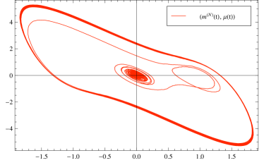
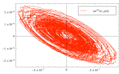
    For intermediate values of σ𝜎\sigma the behavior depends on the parameters. The most interesting case is for θ1<θ<α+2subscript𝜃1𝜃𝛼2\theta_{1}<\theta<\alpha+2. By increasing σ𝜎\sigma, the basin of attraction of the invariant law (4.2) shrinks, and this invariant law becomes unstable at a critical value σ=σc𝜎subscript𝜎𝑐\sigma=\sigma_{c}. A unique stable periodic solution survives for σ<σc𝜎subscriptsuperscript𝜎𝑐\sigma<\sigma^{\prime}_{c}, with σc>σcsubscriptsuperscript𝜎𝑐subscript𝜎𝑐\sigma^{\prime}_{c}>\sigma_{c}. Thus, an initial condition that, for small σ𝜎\sigma, would be in the basin of attraction of (4.2), gets excited by the noise, and is attracted by a periodic orbit. See Figure 1.
Refer to caption
Refer to caption
Figure 1: The figures illustrate the phenomenon of excitation by noise, that is how noise (of suitable intensity) helps/favors the emergence of a stable periodic behavior. Simulations of the interacting particle system (3.2) have been run for θ𝜃\theta slightly below the threshold value α+2𝛼2\alpha+2. Recall that this range of the parameter corresponds to a coexistence phase for the deterministic system (4.3), in which the locally stable equilibria (±1,0)plus-or-minus10(\pm 1,0) coexist with a macroscopic stable limit cycle. We simulate the trajectory t(m(N)(t),μ(t))maps-to𝑡superscript𝑚𝑁𝑡𝜇𝑡t\mapsto(m^{(N)}(t),\mu(t)) for different noise sizes. Both simulations are performed for the same number of iterations, with the same time-step size, and starting from (m(N)(0),μ(0))=(0,0)superscript𝑚𝑁0𝜇000(m^{(N)}(0),\mu(0))=(0,0) with particles initially placed half in (+1,0)10(+1,0) and half in (1,0)10(-1,0). Only the noise size is changing. On the left panel, when σ𝜎\sigma is small, the curve (m(N)(t),μ(t))superscript𝑚𝑁𝑡𝜇𝑡(m^{(N)}(t),\mu(t)) stays close to the initial point for all times; indeed, it oscillates with maximum amplitude of order of 106superscript10610^{-6}. On the right panel, we increase the noise size and (m(N)(t),μ(t))superscript𝑚𝑁𝑡𝜇𝑡(m^{(N)}(t),\mu(t)) exhibits a periodic behavior.

We have no proof of the above statements, but strong evidences is obtained through numerical simulations. Surprisingly, even the analysis of the linear stability of (4.2) appears to be quite hard. One possible approach consists in considering the infinite dimensional system of equations for the moments of (3.4). By Ito’s rule we obtain, for k1𝑘1k\geq 1:

dxk(t)=[kxk+2(t)+kxk(t)+σ22k(k1)xk2(t)kμ(t)xk1(t)]dt+σkxk1(t)dB(t).𝑑superscript𝑥𝑘𝑡delimited-[]𝑘superscript𝑥𝑘2𝑡𝑘superscript𝑥𝑘𝑡superscript𝜎22𝑘𝑘1superscript𝑥𝑘2𝑡𝑘𝜇𝑡superscript𝑥𝑘1𝑡𝑑𝑡𝜎𝑘superscript𝑥𝑘1𝑡𝑑𝐵𝑡dx^{k}(t)=\left[-kx^{k+2}(t)+kx^{k}(t)+\frac{\sigma^{2}}{2}k(k-1)x^{k-2}(t)-k\mu(t)x^{k-1}(t)\right]dt+\sigma kx^{k-1}(t)dB(t)\,.

Setting mk(t):=𝔼(xk(t))assignsubscript𝑚𝑘𝑡𝔼superscript𝑥𝑘𝑡m_{k}(t):={\mathbb{E}}(x^{k}(t)), taking the expectation in the previous equation we get

dmkdt(t)=kmk+2(t)+kmk(t)+σ22k(k1)mk2(t)kμ(t)mk1(t)dμdt(t)=(αθ)μ(t)θ(m3(t)+m1(t))=αμ(t)θdm1(t)dt.𝑑subscript𝑚𝑘𝑑𝑡𝑡𝑘subscript𝑚𝑘2𝑡𝑘subscript𝑚𝑘𝑡superscript𝜎22𝑘𝑘1subscript𝑚𝑘2𝑡𝑘𝜇𝑡subscript𝑚𝑘1𝑡𝑑𝜇𝑑𝑡𝑡𝛼𝜃𝜇𝑡𝜃subscript𝑚3𝑡subscript𝑚1𝑡𝛼𝜇𝑡𝜃𝑑subscript𝑚1𝑡𝑑𝑡\begin{split}\dfrac{dm_{k}}{dt}(t)&=-km_{k+2}(t)+km_{k}(t)+\dfrac{\sigma^{2}}{2}k(k-1)m_{k-2}(t)-k\mu(t)m_{k-1}(t)\\ \frac{d\mu}{dt}(t)&=-(\alpha-\theta)\mu(t)-\theta\left(-m_{3}(t)+m_{1}(t)\right)=-\alpha\mu(t)-\theta\dfrac{dm_{1}(t)}{dt}.\end{split} (4.4)

This system of equations appears to be as hard as (4.1). However, we use it as a guide to construct a Gaussian approximation of (3.4). To be precise, denote by (xσ(t),μσ(t))subscript𝑥𝜎𝑡subscript𝜇𝜎𝑡(x_{\sigma}(t),\mu_{\sigma}(t)) the solution of (3.4), for a given deterministic initial condition xσ(0)=x,μσ(0)=μformulae-sequencesubscript𝑥𝜎0𝑥subscript𝜇𝜎0𝜇x_{\sigma}(0)=x,\mu_{\sigma}(0)=\mu (random initial conditions could be considered as well). We construct, on the same probability space, a process (yσ(t),νσ(t))subscript𝑦𝜎𝑡subscript𝜈𝜎𝑡(y_{\sigma}(t),\nu_{\sigma}(t)) satisfying the following conditions:

  • (a)

    yσ()subscript𝑦𝜎y_{\sigma}(\cdot) is a Gauss-Markov process, νσ()subscript𝜈𝜎\nu_{\sigma}(\cdot) is a deterministic process, yσ(0)=xsubscript𝑦𝜎0𝑥y_{\sigma}(0)=x, νσ(0)=μsubscript𝜈𝜎0𝜇\nu_{\sigma}(0)=\mu.

  • (b)

    The moments of yσ()subscript𝑦𝜎y_{\sigma}(\cdot) and νσ()subscript𝜈𝜎\nu_{\sigma}(\cdot) satisfy (4.4) for k=1,2𝑘12k=1,2.

  • (c)

    For every T>0𝑇0T>0 there is a constant CTsubscript𝐶𝑇C_{T} such that for all σ>0𝜎0\sigma>0

    𝔼[supt[0,T]|xσ(t)yσ(t)|]+supt[0,T]|μσ(t)νσ(t)|CTσ2.𝔼delimited-[]subscriptsupremum𝑡0𝑇subscript𝑥𝜎𝑡subscript𝑦𝜎𝑡subscriptsupremum𝑡0𝑇subscript𝜇𝜎𝑡subscript𝜈𝜎𝑡subscript𝐶𝑇superscript𝜎2{\mathbb{E}}\left[\sup_{t\in[0,T]}|x_{\sigma}(t)-y_{\sigma}(t)|\right]+\sup_{t\in[0,T]}|\mu_{\sigma}(t)-\nu_{\sigma}(t)|\leq C_{T}\sigma^{2}. (4.5)

Note that (4.5), which expresses the fact that yσsubscript𝑦𝜎y_{\sigma} is a small noise approximation of xσsubscript𝑥𝜎x_{\sigma}, is not enough to identify the law of yσsubscript𝑦𝜎y_{\sigma}, since this condition in insensitive to corrections of order σ2superscript𝜎2\sigma^{2}. These corrections are determined by condition (b); indeed, the equations (4.4) for k=1,2𝑘12k=1,2 form a closed system of two equations, since for Gaussian random variables, all moments can be expressed in terms of the first two.

We now define the Gaussian process yσsubscript𝑦𝜎y_{\sigma}. First, consider the following system of ODEs:

dmσdt=mσ3+mσνσ3σ2mσVσdνσdt=ανσθdmσdtdVσdt=1+2(13mσ2)Vσ6σ2Vσ2mσ(0)=xνσ(0)=μVσ(0)=0.formulae-sequence𝑑subscript𝑚𝜎𝑑𝑡superscriptsubscript𝑚𝜎3subscript𝑚𝜎subscript𝜈𝜎3superscript𝜎2subscript𝑚𝜎subscript𝑉𝜎𝑑subscript𝜈𝜎𝑑𝑡𝛼subscript𝜈𝜎𝜃𝑑subscript𝑚𝜎𝑑𝑡𝑑subscript𝑉𝜎𝑑𝑡1213superscriptsubscript𝑚𝜎2subscript𝑉𝜎6superscript𝜎2superscriptsubscript𝑉𝜎2subscript𝑚𝜎0𝑥formulae-sequencesubscript𝜈𝜎0𝜇subscript𝑉𝜎00\begin{split}\frac{dm_{\sigma}}{dt}&=-m_{\sigma}^{3}+m_{\sigma}-\nu_{\sigma}-3\sigma^{2}m_{\sigma}V_{\sigma}\\ \frac{d\nu_{\sigma}}{dt}&=-\alpha\nu_{\sigma}-\theta\frac{dm_{\sigma}}{dt}\\ \frac{dV_{\sigma}}{dt}&=1+2(1-3m_{\sigma}^{2})V_{\sigma}-6\sigma^{2}V_{\sigma}^{2}\\ m_{\sigma}(0)&=x\ \ \ \nu_{\sigma}(0)=\mu\ \ \ V_{\sigma}(0)=0.\end{split} (4.6)

It is easily seen that solutions of (4.6) are bounded, which implies global existence and uniqueness. We can therefore define the following Gauss-Markov, centered process, as the unique solution of the linear SDE:

dzσ(t)=[13mσ2(t)3σ2Vσ(t)]zσ(t)dt+dB(t)zσ(0)=0,𝑑subscript𝑧𝜎𝑡delimited-[]13superscriptsubscript𝑚𝜎2𝑡3superscript𝜎2subscript𝑉𝜎𝑡subscript𝑧𝜎𝑡𝑑𝑡𝑑𝐵𝑡subscript𝑧𝜎00\begin{split}dz_{\sigma}(t)&=\left[1-3m_{\sigma}^{2}(t)-3\sigma^{2}V_{\sigma}(t)\right]z_{\sigma}(t)dt+dB(t)\\ z_{\sigma}(0)&=0,\end{split} (4.7)

where B(t)𝐵𝑡B(t) is the same Brownian motion driving (3.4). By computing dzσ2𝑑superscriptsubscript𝑧𝜎2dz_{\sigma}^{2} one checks that

Var(zσ(t))=Vσ(t).𝑉𝑎𝑟subscript𝑧𝜎𝑡subscript𝑉𝜎𝑡Var(z_{\sigma}(t))=V_{\sigma}(t).

Finally, let

yσ(t):=mσ(t)+σzσ(t).assignsubscript𝑦𝜎𝑡subscript𝑚𝜎𝑡𝜎subscript𝑧𝜎𝑡y_{\sigma}(t):=m_{\sigma}(t)+\sigma z_{\sigma}(t). (4.8)
Proposition 6.

Properties (a), (b) and (c) hold for the process yσsubscript𝑦𝜎y_{\sigma} defined in (4.8).

Having obtained a small noise Gaussian approximation for (3.4), we study the approximated process. Being Gaussian, it is enough to study the evolution of mean and variance. Since 𝔼(yσ(t))=mσ(t)𝔼subscript𝑦𝜎𝑡subscript𝑚𝜎𝑡{\mathbb{E}}(y_{\sigma}(t))=m_{\sigma}(t) and Var(yσ(t))=σ2Vσ(t)𝑉𝑎𝑟subscript𝑦𝜎𝑡superscript𝜎2subscript𝑉𝜎𝑡Var(y_{\sigma}(t))=\sigma^{2}V_{\sigma}(t), we are left to the analysis of the three dimensional system (4.6). In the following analysis we omit the subscript σ𝜎\sigma in mσ,νσ,Vσsubscript𝑚𝜎subscript𝜈𝜎subscript𝑉𝜎m_{\sigma},\nu_{\sigma},V_{\sigma}. In the three dimensional space {(m,ν,V):m,ν,V0}conditional-set𝑚𝜈𝑉formulae-sequence𝑚𝜈𝑉0\{(m,\nu,V):\,m,\nu\in{\mathbb{R}},\,V\geq 0\}, equations (4.6) admit the following equilibrium points:

s1=(1+13σ22, 0,113σ26σ2),s2=(1+13σ22, 0,113σ26σ2),formulae-sequencesubscript𝑠1113superscript𝜎22 0113superscript𝜎26superscript𝜎2subscript𝑠2113superscript𝜎22 0113superscript𝜎26superscript𝜎2s_{1}=\left(\frac{\sqrt{1+\sqrt{1-3\sigma^{2}}}}{\sqrt{2}},\>0,\>\frac{1-\sqrt{1-3\sigma^{2}}}{6\sigma^{2}}\right),\quad s_{2}=\left(-\frac{\sqrt{1+\sqrt{1-3\sigma^{2}}}}{\sqrt{2}},\>0,\>\frac{1-\sqrt{1-3\sigma^{2}}}{6\sigma^{2}}\right),
s3=(113σ22, 0,1+13σ26σ2),s4=(113σ22, 0,1+13σ26σ2),formulae-sequencesubscript𝑠3113superscript𝜎22 0113superscript𝜎26superscript𝜎2subscript𝑠4113superscript𝜎22 0113superscript𝜎26superscript𝜎2s_{3}=\left(-\frac{\sqrt{1-\sqrt{1-3\sigma^{2}}}}{\sqrt{2}},\>0,\>\frac{1+\sqrt{1-3\sigma^{2}}}{6\sigma^{2}}\right),\quad s_{4}=\left(\frac{\sqrt{1-\sqrt{1-3\sigma^{2}}}}{\sqrt{2}},\>0,\>\frac{1+\sqrt{1-3\sigma^{2}}}{6\sigma^{2}}\right),

for σ21/3superscript𝜎213\sigma^{2}\leq 1/3, and

s5=(0, 0,1+1+6σ26σ2)subscript𝑠50 0116superscript𝜎26superscript𝜎2s_{5}=\left(0,\>0,\>\frac{1+\sqrt{1+6\sigma^{2}}}{6\sigma^{2}}\right)

for all σ>0𝜎0\sigma>0. Note that, as σ0𝜎0\sigma\downarrow 0, the equilibria s1subscript𝑠1s_{1} and s2subscript𝑠2s_{2} converge to (±1,0,3/2)plus-or-minus1032(\pm 1,0,3/2), so they correspond to the equilibria (±1,0)plus-or-minus10(\pm 1,0) of the deterministic system (4.3); the equilibria s3subscript𝑠3s_{3}, s4subscript𝑠4s_{4}, and s5subscript𝑠5s_{5} converge to (0,0,+)00(0,0,+\infty). In the following result we give a local version of the property of excitability by noise: under suitable conditions on the parameters, by increasing σ𝜎\sigma the equilibria s1subscript𝑠1s_{1} and s2subscript𝑠2s_{2} lose stability.

Theorem 7.

Assume θ<α+2𝜃𝛼2\theta<\alpha+2, with α+2θ𝛼2𝜃\alpha+2-\theta sufficiently small, and assume α<10𝛼10\alpha<10. Then there exists σc>0subscript𝜎𝑐0\sigma_{c}>0 such that s1subscript𝑠1s_{1} and s2subscript𝑠2s_{2} are linearly stable for σ<σc𝜎subscript𝜎𝑐\sigma<\sigma_{c}, but linear stability is lost as σ𝜎\sigma crosses σcsubscript𝜎𝑐\sigma_{c}.

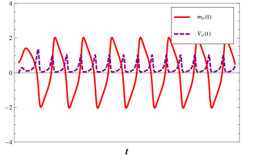
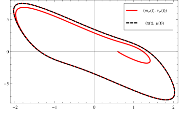
For θ>α+2𝜃𝛼2\theta>\alpha+2 and σ1much-less-than𝜎1\sigma\ll 1, we expect system (4.6) to have an unique attracting periodic solution, as the deterministic system (4.3) has. This behavior is illustrated by simulations in Figure 2.
Refer to caption
Refer to caption
Figure 2: Regime σ1much-less-than𝜎1\sigma\ll 1 and θ>α+2𝜃𝛼2\theta>\alpha+2. In the left panel the (Vσ=0)subscript𝑉𝜎0(V_{\sigma}=0)–section of the typical motion of (mσ,νσ)subscript𝑚𝜎subscript𝜈𝜎(m_{\sigma},\nu_{\sigma}) is shown. The trajectory t(mσ(t),νσ(t))maps-to𝑡subscript𝑚𝜎𝑡subscript𝜈𝜎𝑡t\mapsto(m_{\sigma}(t),\nu_{\sigma}(t)) (solid red line) approaches and remains close to the limit cycle attractor for the dynamics (4.3) (dashed black line). A heuristic explanation of the phenomenon can be inferred from the right panel, where the oscillatory behavior of mσsubscript𝑚𝜎m_{\sigma} and Vσsubscript𝑉𝜎V_{\sigma} is illustrated. Since Vσsubscript𝑉𝜎V_{\sigma} is of order one for all times, the terms proportional to σ2Vσsuperscript𝜎2subscript𝑉𝜎\sigma^{2}V_{\sigma} in (4.6) are small when σ1much-less-than𝜎1\sigma\ll 1. Thus, the trajectories of (4.6) are close to those of the deterministic system (4.3).

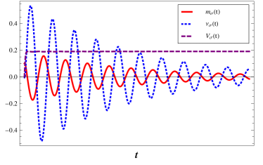
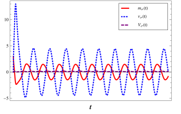
The behavior of (4.6) for large σ𝜎\sigma could be studied as well, although it may not reflect any of the features of (3.4). For θ>α+2𝜃𝛼2\theta>\alpha+2 one shows, in particular, that the equilibrium s5subscript𝑠5s_{5} becomes linearly stable as σ>23(αθ)(αθ1)𝜎23𝛼𝜃𝛼𝜃1\sigma>\sqrt{\frac{2}{3}(\alpha-\theta)(\alpha-\theta-1)}, but it is not a global attractor, since a locally stable periodic orbit survives. This is illustrated in Figure 3.
Refer to caption
Refer to caption
Figure 3: Simulations for the system (4.6) in the case when θ>α+2𝜃𝛼2\theta>\alpha+2 and σ>23(αθ)(αθ1)𝜎23𝛼𝜃𝛼𝜃1\sigma>\sqrt{\frac{2}{3}(\alpha-\theta)(\alpha-\theta-1)}. In this regime the limiting behavior of the trajectories depends on the initial value of the magnetization. We run simulations with starting point Vσ(0)=νσ(0)=0subscript𝑉𝜎0subscript𝜈𝜎00V_{\sigma}(0)=\nu_{\sigma}(0)=0 and various initial conditions for mσ(0)subscript𝑚𝜎0m_{\sigma}(0). For |mσ(0)|1much-less-thansubscript𝑚𝜎01\left|m_{\sigma}(0)\right|\ll 1 the oscillatory behavior disappears. Indeed, (mσ,νσ,Vσ)subscript𝑚𝜎subscript𝜈𝜎subscript𝑉𝜎(m_{\sigma},\nu_{\sigma},V_{\sigma}) converges to s5=(0,0,1+1+6σ26σ2)subscript𝑠500116superscript𝜎26superscript𝜎2s_{5}=(0,0,\frac{1+\sqrt{1+6\sigma^{2}}}{6\sigma^{2}}), which is the only fixed point for the dynamics (4.6) in this phase and is linearly stable (left panel). On the contrary, when |mσ(0)|subscript𝑚𝜎0\left|m_{\sigma}(0)\right| is large, the periodicity persists also for σ1much-greater-than𝜎1\sigma\gg 1 (right panel).

5 Proofs

5.1 Proof of Proposition 4

In view of dynamics (4.1), an equilibrium probability density for our system must satisfy the system of equations

σ22xx2q(x)x{[x3+xμ]q(x)}=0superscript𝜎22subscriptsuperscript2𝑥𝑥subscript𝑞𝑥subscript𝑥delimited-[]superscript𝑥3𝑥subscript𝜇subscript𝑞𝑥0\frac{\sigma^{2}}{2}\partial^{2}_{xx}q_{*}(x)-\partial_{x}\left\{\left[-x^{3}+x-\mu_{*}\right]q_{*}(x)\right\}=0 (5.1a)
(αθ)μθx3+x,q=0.𝛼𝜃subscript𝜇𝜃superscript𝑥3𝑥subscript𝑞0-(\alpha-\theta)\mu_{*}-\theta\left\langle-x^{3}+x,q_{*}\right\rangle=0\,. (5.1b)

Solving (5.1a) we obtain

q(x)=Z1exp{1σ2[x42+x2+2θμx]}subscript𝑞𝑥superscriptsubscript𝑍11superscript𝜎2delimited-[]superscript𝑥42superscript𝑥22𝜃subscript𝜇𝑥q_{*}(x)=Z_{*}^{-1}\cdot\exp\left\{\frac{1}{\sigma^{2}}\left[-\frac{x^{4}}{2}+x^{2}+2\theta\mu_{*}x\right]\right\}

with

Z=exp{1σ2[x42+x2+2θμx]}𝑑x.subscript𝑍subscript1superscript𝜎2delimited-[]superscript𝑥42superscript𝑥22𝜃subscript𝜇𝑥differential-d𝑥Z_{*}=\int_{\mathbb{R}}\exp\left\{\frac{1}{\sigma^{2}}\left[-\frac{x^{4}}{2}+x^{2}+2\theta\mu_{*}x\right]\right\}dx\,.

This result together with equation (5.1b) imply μ=0subscript𝜇0\mu_{*}=0 and the proof is complete.

5.2 Proof of Theorem 5

The scenario depicted in the statement is due to the occurrence of both a homoclinic and a Hopf bifurcation. To ease the readability of the proof, we believe it is worth first to explain what is going on and then to give the technical details.
Roughly speaking, the theorem states there exist three possible phases for system (4.3):

  • 1.

    Fixed points phase. For θ<θ1𝜃subscript𝜃1\theta<\theta_{1} the only stable attractors are (±1,0)plus-or-minus10(\pm 1,0).

  • 2.

    Coexistence phase. For θ=θ1𝜃subscript𝜃1\theta=\theta_{1} the system has an eight-shaped, symmetric with respect to the origin, homoclinic orbit surrounding (±1,0)plus-or-minus10(\pm 1,0). By increasing the parameter θ𝜃\theta from θ1subscript𝜃1\theta_{1}, this separatrix splits into an outer stable limit cycle, which contains both the equilibria, and two inner unstable periodic orbits around (1,0)10(1,0) and (1,0)10(-1,0), respectively. In this phase (±1,0)plus-or-minus10(\pm 1,0) are linearly stable. Therefore, two locally stable fixed points coexist with a stable limit cycle.

  • 3.

    Periodic orbit phase. For θ=α+2𝜃𝛼2\theta=\alpha+2 a Hopf bifurcation occurs: the inner unstable limit cycles disappear collapsing at (±1,0)plus-or-minus10(\pm 1,0). At the same time the equilibria lose their stability and, thus, the external stable limit cycle remains the only stable attractor for θα+2𝜃𝛼2\theta\geq\alpha+2.

The key point of the proof is the particular structure of the vector field generated by (4.3). For convenience, let us denote such a vector field by

Vα,θ(x,μ):=(x3+xμ(αθ)μ+θ(x3x)).assignsubscript𝑉𝛼𝜃𝑥𝜇matrixsuperscript𝑥3𝑥𝜇𝛼𝜃𝜇𝜃superscript𝑥3𝑥V_{\alpha,\theta}(x,\mu):=\begin{pmatrix}-x^{3}+x-\mu\\ -(\alpha-\theta)\mu+\theta(x^{3}-x)\end{pmatrix}. (5.2)

Observe that (5.2) defines a one-parameter family of negatively rotated vector fields (with respect to θ𝜃\theta, for fixed α𝛼\alpha); that is, the following are satisfied

  • 1.

    the critical points of (5.2) are isolated;

  • 2.

    at ordinary points, as the parameter θ𝜃\theta increases, all the field vectors Vα,θ(x,μ)subscript𝑉𝛼𝜃𝑥𝜇V_{\alpha,\theta}(x,\mu) rotate clockwise.

Additionally, (5.2) is semi-complete; in other words, the field rotates of an angle π𝜋\pi as the parameter θ𝜃\theta varies over \mathbb{R}.
For dynamical systems that depend on this specific way on a parameter, many results concerning bifurcations, stability and global behavior of limit cycles and separatrix curves are known. For the sake of completeness and readability, we collect here the properties satisfied by (5.2) that are crucial in the sequel, referring to [10, Chapter 4] for precise and general statements.

  1. 1.

    Limit cycles expand or contract monotonically as the parameter θ𝜃\theta varies in a fixed sense.

  2. 2.

    A limit cycle is generated/absorbed either by a critical point or by a separatrix of (5.2).

  3. 3.

    Cycles of distinct fields do not intersect.

Now let us go into the details of the proof.

Lyapunov function

Let α,θ>0𝛼𝜃0\alpha,\theta>0. Consider the function

W(x,μ)=x22+(θx+μ)22αθ𝑊𝑥𝜇superscript𝑥22superscript𝜃𝑥𝜇22𝛼𝜃W(x,\mu)=\frac{x^{2}}{2}+\frac{(\theta x+\mu)^{2}}{2\alpha\theta}

and observe that the total derivative

ddtW(x,μ)=x4+(1+θ)x21θ(θx+μ)2𝑑𝑑𝑡𝑊𝑥𝜇superscript𝑥41𝜃superscript𝑥21𝜃superscript𝜃𝑥𝜇2\frac{d}{dt}W(x,\mu)=-x^{4}+(1+\theta)x^{2}-\frac{1}{\theta}(\theta x+\mu)^{2}

is negative for every μ𝜇\mu and sufficiently large x𝑥x. Thus, there exists a stable domain for the flux of (4.3) and, in particular, the trajectories can not escape to infinity as t+𝑡t\to+\infty.

Local analysis of equilibria and Hopf bifurcation

As already mentioned, the vector field (5.2) admits three fixed points in the phase plane (x,μ)𝑥𝜇(x,\mu): (0,0)00(0,0) and (±1,0)plus-or-minus10(\pm 1,0). The origin is a saddle point for all values of the parameters; while, the equilibria (±1,0)plus-or-minus10(\pm 1,0) are linearly stable for θ<α+2𝜃𝛼2\theta<\alpha+2 and their local stability is lost for θ>α+2𝜃𝛼2\theta>\alpha+2. At the critical point θ=α+2𝜃𝛼2\theta=\alpha+2 a Hopf bifurcation occurs: by decreasing the parameter θ𝜃\theta from α+2𝛼2\alpha+2 two symmetric unstable limit cycles are generated from (±1,0)plus-or-minus10(\pm 1,0). This proves the first assertion in statement (d).

Separatrix formation and stability

Properties 1 and 2 allow us to explain the appearance of a separatrix curve, whose breakdown causes a homoclinic bifurcation at θ=θ1𝜃subscript𝜃1\theta=\theta_{1}. Indeed, while decreasing θ𝜃\theta from α+2𝛼2\alpha+2, the cycles arisen from (±1,0)plus-or-minus10(\pm 1,0) expand until they join each other at the origin forming a homoclinic eight-shaped separatrix graphic Γ0subscriptΓ0\Gamma_{0} at θ=θ1𝜃subscript𝜃1\theta=\theta_{1}. Notice that, for θ=θ1𝜃subscript𝜃1\theta=\theta_{1}, Γ0=WsubscriptΓ0𝑊\Gamma_{0}=W. This proves statement (b).

Furthermore the exterior of the separatrix is stable. In fact, the existence of a stable domain for the flux of (4.3) implies that all trajectories in an outer neighborhood of Γ0subscriptΓ0\Gamma_{0} approach Γ0subscriptΓ0\Gamma_{0} itself as t+𝑡t\to+\infty.

Description of the phases

We are left to prove statements (a), (c) and part of (d). Hence,

  • (c)

    When the separatrix graphic Γ0subscriptΓ0\Gamma_{0} splits increasing θ𝜃\theta from θ1subscript𝜃1\theta_{1}, it generates a periodic orbit surrounding both (±1,0)plus-or-minus10(\pm 1,0) on its exterior and two smaller limit cycles, around (1,0)10(-1,0) and (1,0)10(1,0) respectively, on its interior.
    The inner cycles are unstable (due to the subcritical Hopf bifurcation at θ=α+2𝜃𝛼2\theta=\alpha+2) and represent the boundaries of the basins of attraction of (±1,0)plus-or-minus10(\pm 1,0). Moreover, the external periodic orbit inherits the stability of the exterior of Γ0subscriptΓ0\Gamma_{0} and so it is stable. See Theorem 2 in [10, Section 4.6] for more details.

  • (a)

    It suffices to prove that in this phase the dynamical system (4.3) does not admit a periodic solution. Indeed, the non-existence of cycles together with the existence of a stable domain for the flux of (4.3) guarantee that every trajectory must converge to an equilibrium as t+𝑡t\to+\infty. The fact that the basins of attraction of (±1,0)plus-or-minus10(\pm 1,0) are separated by W𝑊W is a consequence of the Stable Manifold theorem (see [10, Section 2.7]).
    Thus, it remains to show that there is no limit cycle for θ<θ1𝜃subscript𝜃1\theta<\theta_{1}. From properties 1 and 2 it follows that, as θ𝜃\theta increases from θ1subscript𝜃1\theta_{1} to infinity, the outer stable limit cycle expands and its motion covers the whole region external to Γ0subscriptΓ0\Gamma_{0}. Similarly, the two unstable cycles contract from the graphic Γ0subscriptΓ0\Gamma_{0} and terminate at the critical points (±1,0)plus-or-minus10(\pm 1,0). As a consequence, for θ>θ1𝜃subscript𝜃1\theta>\theta_{1} the entire phase space is covered by expanding or contracting limit cycles. Now, by using property 3, we can deduce that no periodic trajectory may exist for θ<θ1𝜃subscript𝜃1\theta<\theta_{1}. In fact, such an orbit would intersect some of the cycles present when θ>θ1𝜃subscript𝜃1\theta>\theta_{1} that is not possible.

  • (d)

    The statement easily follows by combining the impossibility of escaping trajectories, the presence of the stable manifold of the origin, the loss of stability of the fixed points (±1,0)plus-or-minus10(\pm 1,0) and the existence of a stable limit cycle as a unique attractor in the phase space.

To conclude, we observe that θ1>0subscript𝜃10\theta_{1}>0. If θ1subscript𝜃1\theta_{1} was negative, for θ=0𝜃0\theta=0 some periodic solution should exist. It is sufficient to show that this is not the case. For θ=0𝜃0\theta=0, the trajectory of μ𝜇\mu in (4.3) is μ(t)=μ(0)eαt𝜇𝑡𝜇0superscript𝑒𝛼𝑡\mu(t)=\mu(0)\,e^{-\alpha t} and clearly excludes the possibility of having limit cycles.

5.3 Proof of Proposition 6

Let zσ(t)subscript𝑧𝜎𝑡z_{\sigma}(t) be the solution of the linear stochastic differential equation (4.7). Clearly zσ()subscript𝑧𝜎z_{\sigma}(\cdot) is a centered Gaussian process, so yσ(t):=mσ(t)+σzσ(t)assignsubscript𝑦𝜎𝑡subscript𝑚𝜎𝑡𝜎subscript𝑧𝜎𝑡y_{\sigma}(t):=m_{\sigma}(t)+\sigma z_{\sigma}(t) is obviously Gaussian, which establish property (a). Moreover 𝔼(yσ(t))=mσ(t)𝔼subscript𝑦𝜎𝑡subscript𝑚𝜎𝑡{\mathbb{E}}(y_{\sigma}(t))=m_{\sigma}(t), and Var(yσ(t))=σ2Vσ(t)𝑉𝑎𝑟subscript𝑦𝜎𝑡superscript𝜎2subscript𝑉𝜎𝑡Var(y_{\sigma}(t))=\sigma^{2}V_{\sigma}(t). Property (b), i.e. the fact that the first two moments of yσ(t)subscript𝑦𝜎𝑡y_{\sigma}(t) and νσ()subscript𝜈𝜎\nu_{\sigma}(\cdot) satisfy (4.4) for k=1,2𝑘12k=1,2, follows from a simple direct computation, that uses equations (4.6), and the fact that

𝔼[yσ3(t)]=mσ3(t)+3σ2mσ(t)Vσ(t),𝔼[yσ4(t)]=mσ4(t)+6σ2mσ2(t)Vσ(t)+3σ4Vσ2(t).formulae-sequence𝔼delimited-[]subscriptsuperscript𝑦3𝜎𝑡subscriptsuperscript𝑚3𝜎𝑡3superscript𝜎2subscript𝑚𝜎𝑡subscript𝑉𝜎𝑡𝔼delimited-[]subscriptsuperscript𝑦4𝜎𝑡subscriptsuperscript𝑚4𝜎𝑡6superscript𝜎2subscriptsuperscript𝑚2𝜎𝑡subscript𝑉𝜎𝑡3superscript𝜎4subscriptsuperscript𝑉2𝜎𝑡{\mathbb{E}}\left[y^{3}_{\sigma}(t)\right]=m^{3}_{\sigma}(t)+3\sigma^{2}m_{\sigma}(t)V_{\sigma}(t),\ \ \ \ {\mathbb{E}}\left[y^{4}_{\sigma}(t)\right]=m^{4}_{\sigma}(t)+6\sigma^{2}m^{2}_{\sigma}(t)V_{\sigma}(t)+3\sigma^{4}V^{2}_{\sigma}(t).

So, we are left with the proof of Property (c). By the first equation in (4.6) and (4.7), we have

dyσ=[mσ3+mσνσ3σ2mσVσ3σmσ2zσ+σzσ3σ3Vσzσ]dt+σdB=[yσ3+yσνσ+3σ2mσ(zσ2Vσ)+σ3(zσ33Vσzσ)]dt+σdB.𝑑subscript𝑦𝜎delimited-[]superscriptsubscript𝑚𝜎3subscript𝑚𝜎subscript𝜈𝜎3superscript𝜎2subscript𝑚𝜎subscript𝑉𝜎3𝜎superscriptsubscript𝑚𝜎2subscript𝑧𝜎𝜎subscript𝑧𝜎3superscript𝜎3subscript𝑉𝜎subscript𝑧𝜎𝑑𝑡𝜎𝑑𝐵delimited-[]superscriptsubscript𝑦𝜎3subscript𝑦𝜎subscript𝜈𝜎3superscript𝜎2subscript𝑚𝜎subscriptsuperscript𝑧2𝜎subscript𝑉𝜎superscript𝜎3superscriptsubscript𝑧𝜎33subscript𝑉𝜎subscript𝑧𝜎𝑑𝑡𝜎𝑑𝐵\begin{split}dy_{\sigma}&=\left[-m_{\sigma}^{3}+m_{\sigma}-\nu_{\sigma}-3\sigma^{2}m_{\sigma}V_{\sigma}-3\sigma m_{\sigma}^{2}z_{\sigma}+\sigma z_{\sigma}-3\sigma^{3}V_{\sigma}z_{\sigma}\right]dt+\sigma dB\\ &=\left[-y_{\sigma}^{3}+y_{\sigma}-\nu_{\sigma}+3\sigma^{2}m_{\sigma}(z^{2}_{\sigma}-V_{\sigma})+\sigma^{3}(z_{\sigma}^{3}-3V_{\sigma}z_{\sigma})\right]dt+\sigma dB.\end{split} (5.3)

By subtracting (5.3) from (3.4), we get

xσ(t)yσ(t)=0t{[yσ3(s)xσ3(s)yσ(s)+xσ(s)]+[νσ(s)μσ(s)]}𝑑sσ20tRσ(s)𝑑s=0t[xσ(s)yσ(s)][1f(s)]𝑑s+0t[νσ(s)μσ(s)]𝑑sσ20tRσ(s)𝑑s,subscript𝑥𝜎𝑡subscript𝑦𝜎𝑡superscriptsubscript0𝑡delimited-[]subscriptsuperscript𝑦3𝜎𝑠subscriptsuperscript𝑥3𝜎𝑠subscript𝑦𝜎𝑠subscript𝑥𝜎𝑠delimited-[]subscript𝜈𝜎𝑠subscript𝜇𝜎𝑠differential-d𝑠superscript𝜎2superscriptsubscript0𝑡subscript𝑅𝜎𝑠differential-d𝑠superscriptsubscript0𝑡delimited-[]subscript𝑥𝜎𝑠subscript𝑦𝜎𝑠delimited-[]1𝑓𝑠differential-d𝑠superscriptsubscript0𝑡delimited-[]subscript𝜈𝜎𝑠subscript𝜇𝜎𝑠differential-d𝑠superscript𝜎2superscriptsubscript0𝑡subscript𝑅𝜎𝑠differential-d𝑠\begin{split}x_{\sigma}(t)-y_{\sigma}(t)&=\int_{0}^{t}\left\{\left[y^{3}_{\sigma}(s)-x^{3}_{\sigma}(s)-y_{\sigma}(s)+x_{\sigma}(s)\right]+\left[\nu_{\sigma}(s)-\mu_{\sigma}(s)\right]\right\}ds-\sigma^{2}\int_{0}^{t}R_{\sigma}(s)ds\\ &=\int_{0}^{t}\left[x_{\sigma}(s)-y_{\sigma}(s)\right][1-f(s)]ds+\int_{0}^{t}\left[\nu_{\sigma}(s)-\mu_{\sigma}(s)\right]ds-\sigma^{2}\int_{0}^{t}R_{\sigma}(s)ds,\end{split} (5.4)

where

Rσ(t):=3mσ(t)(zσ2(t)Vσ(t))+σ(zσ3(t)3Vσ(t)zσ(t))assignsubscript𝑅𝜎𝑡3subscript𝑚𝜎𝑡subscriptsuperscript𝑧2𝜎𝑡subscript𝑉𝜎𝑡𝜎superscriptsubscript𝑧𝜎3𝑡3subscript𝑉𝜎𝑡subscript𝑧𝜎𝑡R_{\sigma}(t):=3m_{\sigma}(t)(z^{2}_{\sigma}(t)-V_{\sigma}(t))+\sigma(z_{\sigma}^{3}(t)-3V_{\sigma}(t)z_{\sigma}(t)) (5.5)

and

f(t):=xσ2(t)+yσ2(t)+xσ(t)yσ(t)0.assign𝑓𝑡superscriptsubscript𝑥𝜎2𝑡subscriptsuperscript𝑦2𝜎𝑡subscript𝑥𝜎𝑡subscript𝑦𝜎𝑡0f(t):=x_{\sigma}^{2}(t)+y^{2}_{\sigma}(t)+x_{\sigma}(t)y_{\sigma}(t)\geq 0.

Note that (5.4) can be seen as a linear differential equation for ψ(t):=xσ(t)yσ(t)assign𝜓𝑡subscript𝑥𝜎𝑡subscript𝑦𝜎𝑡\psi(t):=x_{\sigma}(t)-y_{\sigma}(t) of the form

ψ(t)=0tA(s)ψ(s)𝑑s+0tB(s)𝑑s,𝜓𝑡superscriptsubscript0𝑡𝐴𝑠𝜓𝑠differential-d𝑠superscriptsubscript0𝑡𝐵𝑠differential-d𝑠\psi(t)=\int_{0}^{t}A(s)\psi(s)ds+\int_{0}^{t}B(s)ds,

with initial condition ψ(0)=0𝜓00\psi(0)=0, whose solution is given by

ψ(t)=0tB(s)exp[stA(r)𝑑r]𝑑s.𝜓𝑡superscriptsubscript0𝑡𝐵𝑠superscriptsubscript𝑠𝑡𝐴𝑟differential-d𝑟differential-d𝑠\psi(t)=\int_{0}^{t}B(s)\exp\left[\int_{s}^{t}A(r)dr\right]ds. (5.6)

This gives

xσ(t)yσ(t)=0test(1f(r))𝑑r[νσ(s)μσ(s)σ2Rσ(s)]𝑑s.subscript𝑥𝜎𝑡subscript𝑦𝜎𝑡superscriptsubscript0𝑡superscript𝑒superscriptsubscript𝑠𝑡1𝑓𝑟differential-d𝑟delimited-[]subscript𝜈𝜎𝑠subscript𝜇𝜎𝑠superscript𝜎2subscript𝑅𝜎𝑠differential-d𝑠x_{\sigma}(t)-y_{\sigma}(t)=\int_{0}^{t}e^{-\int_{s}^{t}(1-f(r))dr}\left[\nu_{\sigma}(s)-\mu_{\sigma}(s)-\sigma^{2}R_{\sigma}(s)\right]ds. (5.7)

On the other hand, by subtracting from the equation ddtνσ(t)=ανσ(t)θddt𝔼(yσ(t))𝑑𝑑𝑡subscript𝜈𝜎𝑡𝛼subscript𝜈𝜎𝑡𝜃𝑑𝑑𝑡𝔼subscript𝑦𝜎𝑡\frac{d}{dt}\nu_{\sigma}(t)=-\alpha\nu_{\sigma}(t)-\theta\frac{d}{dt}{\mathbb{E}}(y_{\sigma}(t)) the corresponding equation for μσsubscript𝜇𝜎\mu_{\sigma}, we obtain

νσ(t)μσ(t)=α0t[νσ(s)μσ(s)]𝑑sθ[𝔼(yσ(t))𝔼(xσ(t))].subscript𝜈𝜎𝑡subscript𝜇𝜎𝑡𝛼superscriptsubscript0𝑡delimited-[]subscript𝜈𝜎𝑠subscript𝜇𝜎𝑠differential-d𝑠𝜃delimited-[]𝔼subscript𝑦𝜎𝑡𝔼subscript𝑥𝜎𝑡\nu_{\sigma}(t)-\mu_{\sigma}(t)=-\alpha\int_{0}^{t}[\nu_{\sigma}(s)-\mu_{\sigma}(s)]ds-\theta[{\mathbb{E}}(y_{\sigma}(t))-{\mathbb{E}}(x_{\sigma}(t))].

This last formula provides an equation for νσ(t)μσ(t)subscript𝜈𝜎𝑡subscript𝜇𝜎𝑡\nu_{\sigma}(t)-\mu_{\sigma}(t) of the form

ψ(t)=0tA(s)ψ(s)𝑑s+C(t),𝜓𝑡superscriptsubscript0𝑡𝐴𝑠𝜓𝑠differential-d𝑠𝐶𝑡\psi(t)=\int_{0}^{t}A(s)\psi(s)ds+C(t),

whose solution is

ψ(t)=C(t)+0tA(s)C(s)exp[stA(r)𝑑r]𝑑s.𝜓𝑡𝐶𝑡superscriptsubscript0𝑡𝐴𝑠𝐶𝑠superscriptsubscript𝑠𝑡𝐴𝑟differential-d𝑟differential-d𝑠\psi(t)=C(t)+\int_{0}^{t}A(s)C(s)\exp\left[\int_{s}^{t}A(r)dr\right]ds. (5.8)

This yields

νσ(t)μσ(t)=θ[𝔼(xσ(t))𝔼(yσ(t))α0teα(ts)[𝔼(xσ(s))𝔼(yσ(s))]𝑑s],subscript𝜈𝜎𝑡subscript𝜇𝜎𝑡𝜃delimited-[]𝔼subscript𝑥𝜎𝑡𝔼subscript𝑦𝜎𝑡𝛼superscriptsubscript0𝑡superscript𝑒𝛼𝑡𝑠delimited-[]𝔼subscript𝑥𝜎𝑠𝔼subscript𝑦𝜎𝑠differential-d𝑠\nu_{\sigma}(t)-\mu_{\sigma}(t)=\theta\left[{\mathbb{E}}(x_{\sigma}(t))-{\mathbb{E}}(y_{\sigma}(t))-\alpha\int_{0}^{t}e^{-\alpha(t-s)}[{\mathbb{E}}(x_{\sigma}(s))-{\mathbb{E}}(y_{\sigma}(s))]ds\right],

from which the following inequality follows:

supt[0,T]|νσ(t)μσ(t)|subscriptsupremum𝑡0𝑇subscript𝜈𝜎𝑡subscript𝜇𝜎𝑡\displaystyle\sup_{t\in[0,T]}|\nu_{\sigma}(t)-\mu_{\sigma}(t)| θsupt[0,T]|𝔼(xσ(t))𝔼(yσ(t))|absent𝜃subscriptsupremum𝑡0𝑇𝔼subscript𝑥𝜎𝑡𝔼subscript𝑦𝜎𝑡\displaystyle\leq\theta\sup_{t\in[0,T]}\left|{\mathbb{E}}(x_{\sigma}(t))-{\mathbb{E}}(y_{\sigma}(t))\right|
αθsupt[0,T]0teα(ts)|𝔼(xσ(s))𝔼(yσ(s))|𝑑s𝛼𝜃subscriptsupremum𝑡0𝑇superscriptsubscript0𝑡superscript𝑒𝛼𝑡𝑠𝔼subscript𝑥𝜎𝑠𝔼subscript𝑦𝜎𝑠differential-d𝑠\displaystyle\qquad-\alpha\theta\sup_{t\in[0,T]}\int_{0}^{t}e^{-\alpha(t-s)}\left|{\mathbb{E}}(x_{\sigma}(s))-{\mathbb{E}}(y_{\sigma}(s))\right|ds
KTsupt[0,T]𝔼[|xσ(t)yσ(t)|],absentsubscript𝐾𝑇subscriptsupremum𝑡0𝑇𝔼delimited-[]subscript𝑥𝜎𝑡subscript𝑦𝜎𝑡\displaystyle\leq K_{T}\sup_{t\in[0,T]}{\mathbb{E}}\left[\left|x_{\sigma}(t)-y_{\sigma}(t)\right|\right], (5.9)

for some constant KT>0subscript𝐾𝑇0K_{T}>0. By (5.7) and (5.3) we get

𝔼[supt[0,T]|xσ(t)yσ(t)|]AT0T𝔼[sups[0,t]|xσ(s)yσ(s)|]𝑑s+ATσ2supt[0,T]𝔼[|Rσ(t)|]𝔼delimited-[]subscriptsupremum𝑡0𝑇subscript𝑥𝜎𝑡subscript𝑦𝜎𝑡subscript𝐴𝑇superscriptsubscript0𝑇𝔼delimited-[]subscriptsupremum𝑠0𝑡subscript𝑥𝜎𝑠subscript𝑦𝜎𝑠differential-d𝑠subscript𝐴𝑇superscript𝜎2subscriptsupremum𝑡0𝑇𝔼delimited-[]subscript𝑅𝜎𝑡{\mathbb{E}}\left[\sup_{t\in[0,T]}\left|x_{\sigma}(t)-y_{\sigma}(t)\right|\right]\leq A_{T}\int_{0}^{T}\mathbb{E}\left[\sup_{s\in[0,t]}\left|x_{\sigma}(s)-y_{\sigma}(s)\right|\right]ds+A_{T}\sigma^{2}\sup_{t\in[0,T]}{\mathbb{E}}\left[\left|R_{\sigma}(t)\right|\right]

for some AT>0subscript𝐴𝑇0A_{T}>0 which, by Gronwall’s Lemma, yields, for all σ𝜎\sigma in a bounded subset of (0,+)0(0,+\infty)

𝔼[supt[0,T]|xσ(t)yσ(t)|]BTσ2supt[0,T]𝔼[|Rσ(t)|]CTσ2,𝔼delimited-[]subscriptsupremum𝑡0𝑇subscript𝑥𝜎𝑡subscript𝑦𝜎𝑡subscript𝐵𝑇superscript𝜎2subscriptsupremum𝑡0𝑇𝔼delimited-[]subscript𝑅𝜎𝑡subscript𝐶𝑇superscript𝜎2{\mathbb{E}}\left[\sup_{t\in[0,T]}\left|x_{\sigma}(t)-y_{\sigma}(t)\right|\right]\leq B_{T}\sigma^{2}\sup_{t\in[0,T]}{\mathbb{E}}\left[\left|R_{\sigma}(t)\right|\right]\leq C_{T}\sigma^{2}, (5.10)

where the last inequality follows from the fact that Rσ(t)subscript𝑅𝜎𝑡R_{\sigma}(t) is a polynomial function of a Gauss-Markov process and, therefore, has a L1superscript𝐿1L^{1}-norm which is locally bounded in time. To complete the proof of (4.5) we still need to show that

supt[0,T]|μσ(t)νσ(t)|CTσ2subscriptsupremum𝑡0𝑇subscript𝜇𝜎𝑡subscript𝜈𝜎𝑡subscript𝐶𝑇superscript𝜎2\sup_{t\in[0,T]}|\mu_{\sigma}(t)-\nu_{\sigma}(t)|\leq C_{T}\sigma^{2}

for some CT>0subscript𝐶𝑇0C_{T}>0, which follows immediately from (5.10) and (5.3).

5.4 Proof of Theorem 7

By symmetry, it is enough to consider the equilibrium s1subscript𝑠1s_{1}. Consider the vector field Vα,θσsuperscriptsubscript𝑉𝛼𝜃𝜎V_{\alpha,\theta}^{\sigma} associated to equation (4.6)

Vα,θσ(m,ν,v):=(m3+mν3σ2mv(αθ)ν+θ(m3m)+3θσ2mv1+2(13m2)v6σ2v2).assignsuperscriptsubscript𝑉𝛼𝜃𝜎𝑚𝜈𝑣superscript𝑚3𝑚𝜈3superscript𝜎2𝑚𝑣𝛼𝜃𝜈𝜃superscript𝑚3𝑚3𝜃superscript𝜎2𝑚𝑣1213superscript𝑚2𝑣6superscript𝜎2superscript𝑣2V_{\alpha,\theta}^{\sigma}(m,\nu,v):=\left(\begin{array}[]{c}-m^{3}+m-\nu-3\sigma^{2}mv\\ -(\alpha-\theta)\nu+\theta(m^{3}-m)+3\theta\sigma^{2}mv\\ 1+2(1-3m^{2})v-6\sigma^{2}v^{2}\end{array}\right).

We linearize the system around s1subscript𝑠1s_{1}; we obtain the linear system associated to the Jacobian matrix

DVα,θσ(s1)=(113σ213σ21+13σ22θ(1+13σ2)α+θ3θσ21+13σ22321+13σ20313σ2).𝐷superscriptsubscript𝑉𝛼𝜃𝜎subscript𝑠1matrix113superscript𝜎213superscript𝜎2113superscript𝜎22𝜃113superscript𝜎2𝛼𝜃3𝜃superscript𝜎2113superscript𝜎2232113superscript𝜎20313superscript𝜎2DV_{\alpha,\theta}^{\sigma}\left(s_{1}\right)=\begin{pmatrix}-1-\sqrt{1-3\sigma^{2}}&-1&3\,\sigma^{2}\dfrac{\sqrt{1+\sqrt{1-3\sigma^{2}}}}{\sqrt{2}}\\ \theta\left(1+\sqrt{1-3\sigma^{2}}\right)&-\alpha+\theta&-3\,\theta\sigma^{2}\dfrac{\sqrt{1+\sqrt{1-3\sigma^{2}}}}{\sqrt{2}}\\ \dfrac{3\sqrt{2}}{\sqrt{1+\sqrt{1-3\sigma^{2}}}}&0&-3-\sqrt{1-3\sigma^{2}}\end{pmatrix}.

In particular, for σ2=0superscript𝜎20\sigma^{2}=0 and θ=α+2𝜃𝛼2\theta=\alpha+2,

DVα,α+20(s1)=(2102(α+2)20304)𝐷superscriptsubscript𝑉𝛼𝛼20subscript𝑠12102𝛼220missing-subexpressionmissing-subexpressionmissing-subexpression304DV_{\alpha,\alpha+2}^{0}\left(s_{1}\right)=\left(\begin{array}[]{cc|c}-2&-1&0\\ 2(\alpha+2)&2&0\\ \hline\cr 3&0&-4\end{array}\right)

whose spectrum is given by

Spec[DVα,α+20(s1)]={4}{±i2α}.Specdelimited-[]𝐷superscriptsubscript𝑉𝛼𝛼20subscript𝑠14plus-or-minus𝑖2𝛼\mathrm{Spec}\left[DV_{\alpha,\alpha+2}^{0}\left(s_{1}\right)\right]=\{-4\}\cup\{\pm i\sqrt{2\alpha}\}\,.

Denote by λ(σ)𝜆𝜎\lambda(\sigma) the continuous function giving an eigenvalue of the matrix DVα,α+2σ(s1)𝐷superscriptsubscript𝑉𝛼𝛼2𝜎subscript𝑠1DV_{\alpha,\alpha+2}^{\sigma}\left(s_{1}\right), with λ(0)=2αi𝜆02𝛼𝑖\lambda(0)=\sqrt{2\alpha}i. We are going to show that, if α<10𝛼10\alpha<10, then

dd(σ2)Re(λ(σ))|σ=0>0.evaluated-at𝑑𝑑superscript𝜎2Re𝜆𝜎𝜎00\frac{d}{d(\sigma^{2})}\mathrm{Re}\left(\lambda(\sigma)\right)\Big{|}_{\sigma=0}>0. (5.11)

It follows that there is σ>0𝜎0\sigma>0 such that the matrix DVα,α+2σ(s1)𝐷superscriptsubscript𝑉𝛼𝛼2𝜎subscript𝑠1DV_{\alpha,\alpha+2}^{\sigma}\left(s_{1}\right) has an eigenvalue with strictly positive real part. By continuity, this implies that if θ<α+2𝜃𝛼2\theta<\alpha+2 but sufficiently close to α+2𝛼2\alpha+2, then also the matrix DVα,θσ(s1)𝐷superscriptsubscript𝑉𝛼𝜃𝜎subscript𝑠1DV_{\alpha,\theta}^{\sigma}\left(s_{1}\right) has an eigenvalue with strictly positive real part, and this suffices to complete the proof. Thus, we are left with the proof of (5.11). We write

0=det(DVα,α+2σ(s1)λ(σ)𝕀)=a0(σ)+a1(σ)λ(σ)+a2(σ)(λ(σ))2+a3(σ)(λ(σ))3,0𝐷superscriptsubscript𝑉𝛼𝛼2𝜎subscript𝑠1𝜆𝜎𝕀subscript𝑎0𝜎subscript𝑎1𝜎𝜆𝜎subscript𝑎2𝜎superscript𝜆𝜎2subscript𝑎3𝜎superscript𝜆𝜎30=\det\left(DV_{\alpha,\alpha+2}^{\sigma}\left(s_{1}\right)-\lambda(\sigma)\mathbb{I}\right)=a_{0}(\sigma)+a_{1}(\sigma)\lambda(\sigma)+a_{2}(\sigma)\left(\lambda(\sigma)\right)^{2}+a_{3}(\sigma)\left(\lambda(\sigma)\right)^{3},

which gives

dd(σ2)(λ(σ))|σ=0=1a1(0)dd(σ2)a0(σ)|σ=0.evaluated-at𝑑𝑑superscript𝜎2𝜆𝜎𝜎0evaluated-at1subscript𝑎10𝑑𝑑superscript𝜎2subscript𝑎0𝜎𝜎0\frac{d}{d(\sigma^{2})}\left(\lambda(\sigma)\right)\Big{|}_{\sigma=0}=\frac{1}{a_{1}(0)}\frac{d}{d(\sigma^{2})}a_{0}(\sigma)\Big{|}_{\sigma=0}.

Since

det(DVα,α+2σ(s1)λ𝕀)=λ32[1+13σ2]λ2+[2α+12σ2(α+2)13σ2]λ4α13σ2(1+13σ2),𝐷superscriptsubscript𝑉𝛼𝛼2𝜎subscript𝑠1𝜆𝕀superscript𝜆32delimited-[]113superscript𝜎2superscript𝜆2delimited-[]2𝛼12superscript𝜎2𝛼213superscript𝜎2𝜆4𝛼13superscript𝜎2113superscript𝜎2\det\left(DV_{\alpha,\alpha+2}^{\sigma}\left(s_{1}\right)-\lambda\mathbb{I}\right)\\ =-\lambda^{3}-2\left[1+\sqrt{1-3\sigma^{2}}\right]\lambda^{2}+\left[2-\alpha+12\sigma^{2}-\left(\alpha+2\right)\sqrt{1-3\sigma^{2}}\right]\lambda\\ -4\alpha\sqrt{1-3\sigma^{2}}\left(1+\sqrt{1-3\sigma^{2}}\right),

we obtain

dd(σ2)(λ(σ))|σ=0=3λ2(0)+3(5+α2)λ(0)+18α3λ2(0)+8λ(0)+2α.evaluated-at𝑑𝑑superscript𝜎2𝜆𝜎𝜎03superscript𝜆2035𝛼2𝜆018𝛼3superscript𝜆208𝜆02𝛼\frac{d}{d(\sigma^{2})}\left(\lambda(\sigma)\right)\Big{|}_{\sigma=0}=\frac{3\lambda^{2}(0)+3\left(5+\frac{\alpha}{2}\right)\lambda(0)+18\alpha}{3\lambda^{2}(0)+8\lambda(0)+2\alpha}.

Inserting λ(0)=2αi𝜆02𝛼𝑖\lambda(0)=\sqrt{2\alpha}i, we easily get

dd(σ2)Re(λ(σ))|σ=0=3(10α)2(8+α),evaluated-at𝑑𝑑superscript𝜎2Re𝜆𝜎𝜎0310𝛼28𝛼\frac{d}{d(\sigma^{2})}\mathrm{Re}\left(\lambda(\sigma)\right)\Big{|}_{\sigma=0}=\frac{3(10-\alpha)}{2(8+\alpha)},

from which (5.11) follows.

6 Appendix

6.1 Proof of Theorem 2

It will be convenient to write (3.4) in the form

dx(t)=(x3(t)+x(t))dtμ(t)dt+σdB(t)dμdt(t)=αμ(t)θddt𝔼[x(t)].𝑑𝑥𝑡superscript𝑥3𝑡𝑥𝑡𝑑𝑡𝜇𝑡𝑑𝑡𝜎𝑑𝐵𝑡𝑑𝜇𝑑𝑡𝑡𝛼𝜇𝑡𝜃𝑑𝑑𝑡𝔼delimited-[]𝑥𝑡\begin{split}dx(t)&=\left(-x^{3}(t)+x(t)\right)dt-\mu(t)dt+\sigma dB(t)\\ \frac{d\mu}{dt}(t)&=-\alpha\mu(t)-\theta\frac{d}{dt}{\mathbb{E}}\left[x(t)\right].\end{split} (6.1)

The second equation in (6.1) can be solved in μ(t)𝜇𝑡\mu(t):

μ(t)=eαtμ0θ𝔼[x(t)]+θeαt𝔼(ξ)+αθ0teα(ts)𝔼[x(s)]𝑑s.𝜇𝑡superscript𝑒𝛼𝑡subscript𝜇0𝜃𝔼delimited-[]𝑥𝑡𝜃superscript𝑒𝛼𝑡𝔼𝜉𝛼𝜃superscriptsubscript0𝑡superscript𝑒𝛼𝑡𝑠𝔼delimited-[]𝑥𝑠differential-d𝑠\mu(t)=e^{-\alpha t}\mu_{0}-\theta{\mathbb{E}}[x(t)]+\theta e^{-\alpha t}{\mathbb{E}}(\xi)+\alpha\theta\int_{0}^{t}e^{-\alpha(t-s)}{\mathbb{E}}[x(s)]ds. (6.2)

To show existence and uniqueness in (6.1) we follow the argument in [2] (Theorem 2.4.1). Given μ0subscript𝜇0\mu_{0}\in{\mathbb{R}}, we define the stochastic processes (xn(t))t0subscriptsubscript𝑥𝑛𝑡𝑡0(x_{n}(t))_{t\geq 0} and the functions (μn(t))t0subscriptsubscript𝜇𝑛𝑡𝑡0(\mu_{n}(t))_{t\geq 0}, for n0𝑛0n\geq 0, by the following Picard iteration:

dxn(t)=(xn3(t)+xn(t))dtμn(t)dt+σdB(t)μn+1(t)=eαtμ0θ𝔼[xn(t)]+θeαt𝔼(ξ)+αθ0teα(ts)𝔼[xn(s)]𝑑s,𝑑subscript𝑥𝑛𝑡superscriptsubscript𝑥𝑛3𝑡subscript𝑥𝑛𝑡𝑑𝑡subscript𝜇𝑛𝑡𝑑𝑡𝜎𝑑𝐵𝑡subscript𝜇𝑛1𝑡superscript𝑒𝛼𝑡subscript𝜇0𝜃𝔼delimited-[]subscript𝑥𝑛𝑡𝜃superscript𝑒𝛼𝑡𝔼𝜉𝛼𝜃superscriptsubscript0𝑡superscript𝑒𝛼𝑡𝑠𝔼delimited-[]subscript𝑥𝑛𝑠differential-d𝑠\begin{split}dx_{n}(t)&=(-x_{n}^{3}(t)+x_{n}(t))dt-\mu_{n}(t)dt+\sigma dB(t)\\ \mu_{n+1}(t)&=e^{-\alpha t}\mu_{0}-\theta{\mathbb{E}}[x_{n}(t)]+\theta e^{-\alpha t}{\mathbb{E}}(\xi)+\alpha\theta\int_{0}^{t}e^{-\alpha(t-s)}{\mathbb{E}}[x_{n}(s)]ds,\end{split} (6.3)

all with the same initial condition xn(0)=ξsubscript𝑥𝑛0𝜉x_{n}(0)=\xi, μn(0)=μ0subscript𝜇𝑛0subscript𝜇0\mu_{n}(0)=\mu_{0}. Setting

f(t):=xn+12(t)+xn2(t)+xn+1(t)xn(t)0,assign𝑓𝑡subscriptsuperscript𝑥2𝑛1𝑡subscriptsuperscript𝑥2𝑛𝑡subscript𝑥𝑛1𝑡subscript𝑥𝑛𝑡0f(t):=x^{2}_{n+1}(t)+x^{2}_{n}(t)+x_{n+1}(t)x_{n}(t)\geq 0,

and observing that

xn+13(t)xn3(t)=(xn+1(t)xn(t))f(t),subscriptsuperscript𝑥3𝑛1𝑡subscriptsuperscript𝑥3𝑛𝑡subscript𝑥𝑛1𝑡subscript𝑥𝑛𝑡𝑓𝑡x^{3}_{n+1}(t)-x^{3}_{n}(t)=(x_{n+1}(t)-x_{n}(t))f(t),

we get

xn+1(t)xn(t)=0t[xn+1(s)xn(s)][1f(s)]𝑑s0t[μn+1(s)μn(s)]𝑑s=0t[xn+1(s)xn(s)][1f(s)]𝑑s+θ0t𝔼[xn(s)xn1(s)]𝑑sαθ0t0seα(sr)𝔼[xn(r)xn1(r)]𝑑r𝑑s.subscript𝑥𝑛1𝑡subscript𝑥𝑛𝑡superscriptsubscript0𝑡delimited-[]subscript𝑥𝑛1𝑠subscript𝑥𝑛𝑠delimited-[]1𝑓𝑠differential-d𝑠superscriptsubscript0𝑡delimited-[]subscript𝜇𝑛1𝑠subscript𝜇𝑛𝑠differential-d𝑠superscriptsubscript0𝑡delimited-[]subscript𝑥𝑛1𝑠subscript𝑥𝑛𝑠delimited-[]1𝑓𝑠differential-d𝑠𝜃superscriptsubscript0𝑡𝔼delimited-[]subscript𝑥𝑛𝑠subscript𝑥𝑛1𝑠differential-d𝑠𝛼𝜃superscriptsubscript0𝑡superscriptsubscript0𝑠superscript𝑒𝛼𝑠𝑟𝔼delimited-[]subscript𝑥𝑛𝑟subscript𝑥𝑛1𝑟differential-d𝑟differential-d𝑠\begin{split}x_{n+1}(t)-x_{n}(t)&=\int_{0}^{t}\left[x_{n+1}(s)-x_{n}(s)\right][1-f(s)]ds-\int_{0}^{t}\left[\mu_{n+1}(s)-\mu_{n}(s)\right]ds\\ &=\int_{0}^{t}\left[x_{n+1}(s)-x_{n}(s)\right][1-f(s)]ds+\theta\int_{0}^{t}{\mathbb{E}}\left[x_{n}(s)-x_{n-1}(s)\right]ds\\ &~{}~{}-\alpha\theta\int_{0}^{t}\int_{0}^{s}e^{-\alpha(s-r)}{\mathbb{E}}\left[x_{n}(r)-x_{n-1}(r)\right]drds.\end{split}

Note that, setting ψ(t):=xn+1(t)xn(t)assign𝜓𝑡subscript𝑥𝑛1𝑡subscript𝑥𝑛𝑡\psi(t):=x_{n+1}(t)-x_{n}(t), as in the proof of Proposition 6, this last identity is of the form of a linear differential equation

ψ(t)=0tA(s)ψ(s)𝑑s+0tB(s)𝑑s,𝜓𝑡superscriptsubscript0𝑡𝐴𝑠𝜓𝑠differential-d𝑠superscriptsubscript0𝑡𝐵𝑠differential-d𝑠\psi(t)=\int_{0}^{t}A(s)\psi(s)ds+\int_{0}^{t}B(s)ds,

whose solution is given by (5.6). This yields

xn+1(t)xn(t)=0test(1f(u))𝑑u[θ𝔼[xn(s)xn1(s)]αθ0seα(sr)𝔼[xn(r)xn1(r)]𝑑r]𝑑s.subscript𝑥𝑛1𝑡subscript𝑥𝑛𝑡superscriptsubscript0𝑡superscript𝑒superscriptsubscript𝑠𝑡1𝑓𝑢differential-d𝑢delimited-[]𝜃𝔼delimited-[]subscript𝑥𝑛𝑠subscript𝑥𝑛1𝑠𝛼𝜃superscriptsubscript0𝑠superscript𝑒𝛼𝑠𝑟𝔼delimited-[]subscript𝑥𝑛𝑟subscript𝑥𝑛1𝑟differential-d𝑟differential-d𝑠x_{n+1}(t)-x_{n}(t)\\ =\int_{0}^{t}e^{\int_{s}^{t}(1-f(u))du}\left[\theta{\mathbb{E}}\left[x_{n}(s)-x_{n-1}(s)\right]-\alpha\theta\int_{0}^{s}e^{-\alpha(s-r)}{\mathbb{E}}\left[x_{n}(r)-x_{n-1}(r)\right]dr\right]ds. (6.4)

Now, set

φn(t):=sups[0,t]𝔼[|xn+1(s)xn(s)|].assignsubscript𝜑𝑛𝑡subscriptsupremum𝑠0𝑡𝔼delimited-[]subscript𝑥𝑛1𝑠subscript𝑥𝑛𝑠\varphi_{n}(t):=\sup_{s\in[0,t]}{\mathbb{E}}\left[|x_{n+1}(s)-x_{n}(s)|\right].

It follows readily from (6.4) that for each T>0𝑇0T>0 there is a constant CT>0subscript𝐶𝑇0C_{T}>0 for which

φn+1(t)CT0Tφn(s)𝑑s,subscript𝜑𝑛1𝑡subscript𝐶𝑇superscriptsubscript0𝑇subscript𝜑𝑛𝑠differential-d𝑠\varphi_{n+1}(t)\leq C_{T}\int_{0}^{T}\varphi_{n}(s)ds,

which implies

φn(T)φ1(T)(CTT)n1(n1)!.subscript𝜑𝑛𝑇subscript𝜑1𝑇superscriptsubscript𝐶𝑇𝑇𝑛1𝑛1\varphi_{n}(T)\leq\varphi_{1}(T)\frac{(C_{T}T)^{n-1}}{(n-1)!}.

As a consequence, the sequence of functions 𝔼[xn()]𝔼delimited-[]subscript𝑥𝑛{\mathbb{E}}[x_{n}(\cdot)] is Cauchy in 𝒞([0,T])𝒞0𝑇\mathcal{C}([0,T]), and therefore it converges to a limit m(t)𝑚𝑡m(t). Let x()𝑥x(\cdot) be the unique solution of

dx(t)=(x3(t)+x(t))dtμ(t)dt+σdB(t)μ(t)=eαtμ0θm(t)+θeαt𝔼(ξ)+αθ0teα(ts)m(s)𝑑s.𝑑𝑥𝑡superscript𝑥3𝑡𝑥𝑡𝑑𝑡𝜇𝑡𝑑𝑡𝜎𝑑𝐵𝑡𝜇𝑡superscript𝑒𝛼𝑡subscript𝜇0𝜃𝑚𝑡𝜃superscript𝑒𝛼𝑡𝔼𝜉𝛼𝜃superscriptsubscript0𝑡superscript𝑒𝛼𝑡𝑠𝑚𝑠differential-d𝑠\begin{split}dx(t)&=\left(-x^{3}(t)+x(t)\right)dt-\mu(t)dt+\sigma dB(t)\\ \mu(t)&=e^{-\alpha t}\mu_{0}-\theta m(t)+\theta e^{-\alpha t}{\mathbb{E}}(\xi)+\alpha\theta\int_{0}^{t}e^{-\alpha(t-s)}m(s)ds.\end{split} (6.5)

By mimicking the above argument one gets

xn+1(t)x(t)=0test(1f(u))𝑑u[θ𝔼[xn(s)x(s)]αθ0seα(sr)𝔼[xn(r)x(r)]𝑑r]𝑑s,subscript𝑥𝑛1𝑡𝑥𝑡superscriptsubscript0𝑡superscript𝑒superscriptsubscript𝑠𝑡1𝑓𝑢differential-d𝑢delimited-[]𝜃𝔼delimited-[]subscript𝑥𝑛𝑠𝑥𝑠𝛼𝜃superscriptsubscript0𝑠superscript𝑒𝛼𝑠𝑟𝔼delimited-[]subscript𝑥𝑛𝑟𝑥𝑟differential-d𝑟differential-d𝑠x_{n+1}(t)-x(t)\\ =\int_{0}^{t}e^{\int_{s}^{t}(1-f(u))du}\left[\theta{\mathbb{E}}\left[x_{n}(s)-x(s)\right]-\alpha\theta\int_{0}^{s}e^{-\alpha(s-r)}{\mathbb{E}}\left[x_{n}(r)-x(r)\right]dr\right]ds, (6.6)

where, now,

f(t):=xn+12(t)+x2(t)+xn+1(t)x(t)0.assign𝑓𝑡subscriptsuperscript𝑥2𝑛1𝑡superscript𝑥2𝑡subscript𝑥𝑛1𝑡𝑥𝑡0f(t):=x^{2}_{n+1}(t)+x^{2}(t)+x_{n+1}(t)x(t)\geq 0.

As before, this implies that 𝔼(xn(t))𝔼(x(t))𝔼subscript𝑥𝑛𝑡𝔼𝑥𝑡{\mathbb{E}}(x_{n}(t))\rightarrow{\mathbb{E}}(x(t)), and thus m(t)=𝔼(x(t))𝑚𝑡𝔼𝑥𝑡m(t)={\mathbb{E}}(x(t)). This proves that x()𝑥x(\cdot) is a solution of (6.1). The very same argument is used to prove uniqueness. Indeed, if y()𝑦y(\cdot) is another solution, we write the integral equation for y(t)x(t)𝑦𝑡𝑥𝑡y(t)-x(t) and show as before that E(x(t))=E(y(t))𝐸𝑥𝑡𝐸𝑦𝑡E(x(t))=E(y(t)) for all t𝑡t. Thus y()𝑦y(\cdot) and x()𝑥x(\cdot) are both solutions of (6.5) with the same m()𝑚m(\cdot) and the same initial conditions, from which x()=y()𝑥𝑦x(\cdot)=y(\cdot) follows.

6.2 Proof of Theorem 3

We follow a coupling method; we refer to [14] for more details on this approach to prove propagation of chaos. Let (ξi)i=1Nsuperscriptsubscriptsubscript𝜉𝑖𝑖1𝑁(\xi_{i})_{i=1}^{N} be independent random variables with law λ𝜆\lambda, and independent of the Brownian motions (wi(t):t0)i=1N(w_{i}(t):t\geq 0)_{i=1}^{N}. Moreover, let (xi(N)(),μ(N)())i=1Nsuperscriptsubscriptsuperscriptsubscript𝑥𝑖𝑁superscript𝜇𝑁𝑖1𝑁(x_{i}^{(N)}(\cdot),\mu^{(N)}(\cdot))_{i=1}^{N} be the solution of (3.3) with an initial condition xi(N)(0)=ξisubscriptsuperscript𝑥𝑁𝑖0subscript𝜉𝑖x^{(N)}_{i}(0)=\xi_{i}, μi(N)(0)=μ0subscriptsuperscript𝜇𝑁𝑖0subscript𝜇0\mu^{(N)}_{i}(0)=\mu_{0}, while (yi(),ν())i=1Nsuperscriptsubscriptsubscript𝑦𝑖𝜈𝑖1𝑁(y_{i}(\cdot),\nu(\cdot))_{i=1}^{N} solve (3.4) with the same initial conditions and B()=wi()𝐵subscript𝑤𝑖B(\cdot)=w_{i}(\cdot). The claim in Theorem 3 is proved if we show that (the apex N𝑁N in xi(N)superscriptsubscript𝑥𝑖𝑁x_{i}^{(N)} is omitted in what follows)

limN+𝔼[supt[0,T]|x1(t)y1(t)|]=0.subscript𝑁𝔼delimited-[]subscriptsupremum𝑡0𝑇subscript𝑥1𝑡subscript𝑦1𝑡0\lim_{N\rightarrow+\infty}{\mathbb{E}}\left[\sup_{t\in[0,T]}|x_{1}(t)-y_{1}(t)|\right]=0. (6.7)

The strategy is analogous to that of the proof of Theorem 2. We first write, for f(t):=x12(t)+y12(t)+x1(t)y1(t)0assign𝑓𝑡superscriptsubscript𝑥12𝑡superscriptsubscript𝑦12𝑡subscript𝑥1𝑡subscript𝑦1𝑡0f(t):=x_{1}^{2}(t)+y_{1}^{2}(t)+x_{1}(t)y_{1}(t)\geq 0:

x1(t)y1(t)=0t[x1(s)y1(s)][1f(s)]𝑑s0t[μ(s)ν(s)]𝑑s,subscript𝑥1𝑡subscript𝑦1𝑡superscriptsubscript0𝑡delimited-[]subscript𝑥1𝑠subscript𝑦1𝑠delimited-[]1𝑓𝑠differential-d𝑠superscriptsubscript0𝑡delimited-[]𝜇𝑠𝜈𝑠differential-d𝑠x_{1}(t)-y_{1}(t)=\int_{0}^{t}[x_{1}(s)-y_{1}(s)][1-f(s)]ds-\int_{0}^{t}[\mu(s)-\nu(s)]ds,

yielding

x1(t)y1(t)=0t[μ(s)ν(s)]exp[st[1f(r)]𝑑r]𝑑s,subscript𝑥1𝑡subscript𝑦1𝑡superscriptsubscript0𝑡delimited-[]𝜇𝑠𝜈𝑠superscriptsubscript𝑠𝑡delimited-[]1𝑓𝑟differential-d𝑟differential-d𝑠x_{1}(t)-y_{1}(t)=\int_{0}^{t}[\mu(s)-\nu(s)]\exp\left[\int_{s}^{t}[1-f(r)]dr\right]ds,

which gives, for all t[0,T]𝑡0𝑇t\in[0,T],

|x1(t)y1(t)|CT0T|μ(s)ν(s)|𝑑ssubscript𝑥1𝑡subscript𝑦1𝑡subscript𝐶𝑇superscriptsubscript0𝑇𝜇𝑠𝜈𝑠differential-d𝑠|x_{1}(t)-y_{1}(t)|\leq C_{T}\int_{0}^{T}|\mu(s)-\nu(s)|ds (6.8)

for some constant CT>0subscript𝐶𝑇0C_{T}>0. In particular, we have

𝔼[supt[0,T]|x1(t)y1(t)|]CT0T𝔼[|μ(s)ν(s)|]𝑑s.𝔼delimited-[]subscriptsupremum𝑡0𝑇subscript𝑥1𝑡subscript𝑦1𝑡subscript𝐶𝑇superscriptsubscript0𝑇𝔼delimited-[]𝜇𝑠𝜈𝑠differential-d𝑠{\mathbb{E}}\left[\sup_{t\in[0,T]}|x_{1}(t)-y_{1}(t)|\right]\leq C_{T}\int_{0}^{T}{\mathbb{E}}[|\mu(s)-\nu(s)|]ds. (6.9)

On the other hand, it holds

μ(t)ν(t)=α0t[μ(s)ν(s)]𝑑sθ[1Ni=1Nxi(t)𝔼[y1(t)](1Ni=1Nxi(0)𝔼[y1(0)])].𝜇𝑡𝜈𝑡𝛼superscriptsubscript0𝑡delimited-[]𝜇𝑠𝜈𝑠differential-d𝑠𝜃delimited-[]1𝑁superscriptsubscript𝑖1𝑁subscript𝑥𝑖𝑡𝔼delimited-[]subscript𝑦1𝑡1𝑁superscriptsubscript𝑖1𝑁subscript𝑥𝑖0𝔼delimited-[]subscript𝑦10\mu(t)-\nu(t)=-\alpha\int_{0}^{t}[\mu(s)-\nu(s)]ds\\ -\theta\left[\frac{1}{N}\sum_{i=1}^{N}x_{i}(t)-{\mathbb{E}}[y_{1}(t)]-\left(\frac{1}{N}\sum_{i=1}^{N}x_{i}(0)-{\mathbb{E}}[y_{1}(0)]\right)\right]. (6.10)

Set

φ(t):=1Ni=1Nxi(t)𝔼[y1(t)](1Ni=1Nxi(0)𝔼[y1(0)]).assign𝜑𝑡1𝑁superscriptsubscript𝑖1𝑁subscript𝑥𝑖𝑡𝔼delimited-[]subscript𝑦1𝑡1𝑁superscriptsubscript𝑖1𝑁subscript𝑥𝑖0𝔼delimited-[]subscript𝑦10\varphi(t):=\frac{1}{N}\sum_{i=1}^{N}x_{i}(t)-{\mathbb{E}}[y_{1}(t)]-\left(\frac{1}{N}\sum_{i=1}^{N}x_{i}(0)-{\mathbb{E}}[y_{1}(0)]\right).

By (5.8),

μ(t)ν(t)=θφ(t)+αθ0tφ(s)eα(ts)𝑑s.𝜇𝑡𝜈𝑡𝜃𝜑𝑡𝛼𝜃superscriptsubscript0𝑡𝜑𝑠superscript𝑒𝛼𝑡𝑠differential-d𝑠\mu(t)-\nu(t)=-\theta\varphi(t)+\alpha\theta\int_{0}^{t}\varphi(s)e^{-\alpha(t-s)}ds. (6.11)

Note that if in the expression of φ(t)𝜑𝑡\varphi(t) we add and subtract 1Ni[yi(t)yi(0)]1𝑁subscript𝑖delimited-[]subscript𝑦𝑖𝑡subscript𝑦𝑖0\frac{1}{N}\sum_{i}[y_{i}(t)-y_{i}(0)], the following estimate follows for s[0,T]𝑠0𝑇s\in[0,T]:

𝔼[|φ(s)|]𝔼delimited-[]𝜑𝑠\displaystyle{\mathbb{E}}\left[|\varphi(s)|\right] 1Ni=1N𝔼[|xi(s)yi(s)|]+1Ni=1N𝔼[|xi(0)yi(0)|]absent1𝑁superscriptsubscript𝑖1𝑁𝔼delimited-[]subscript𝑥𝑖𝑠subscript𝑦𝑖𝑠1𝑁superscriptsubscript𝑖1𝑁𝔼delimited-[]subscript𝑥𝑖0subscript𝑦𝑖0\displaystyle\leq\frac{1}{N}\sum_{i=1}^{N}{\mathbb{E}}[|x_{i}(s)-y_{i}(s)|]+\frac{1}{N}\sum_{i=1}^{N}{\mathbb{E}}[|x_{i}(0)-y_{i}(0)|]
+𝔼[|1Ni=1Nyi(s)𝔼[y1(s)]|]+𝔼[|1Ni=1Nyi(0)𝔼[y1(0)]|]𝔼delimited-[]1𝑁superscriptsubscript𝑖1𝑁subscript𝑦𝑖𝑠𝔼delimited-[]subscript𝑦1𝑠𝔼delimited-[]1𝑁superscriptsubscript𝑖1𝑁subscript𝑦𝑖0𝔼delimited-[]subscript𝑦10\displaystyle\quad+{\mathbb{E}}\left[\left|\frac{1}{N}\sum_{i=1}^{N}y_{i}(s)-{\mathbb{E}}[y_{1}(s)]\right|\right]+{\mathbb{E}}\left[\left|\frac{1}{N}\sum_{i=1}^{N}y_{i}(0)-{\mathbb{E}}[y_{1}(0)]\right|\right]
𝔼[supr[0,s]|x1(r)y1(r)|]+CN,absent𝔼delimited-[]subscriptsupremum𝑟0𝑠subscript𝑥1𝑟subscript𝑦1𝑟𝐶𝑁\displaystyle\leq{\mathbb{E}}\left[\sup_{r\in[0,s]}|x_{1}(r)-y_{1}(r)|\right]+\frac{C}{\sqrt{N}}, (6.12)

for some C>0𝐶0C>0, where the last inequality follows from the fact that 𝔼[|xi(t)yi(t)|]𝔼delimited-[]subscript𝑥𝑖𝑡subscript𝑦𝑖𝑡{\mathbb{E}}[|x_{i}(t)-y_{i}(t)|] does not depend on i𝑖i, and that the random variables yi(s)subscript𝑦𝑖𝑠y_{i}(s) are i.i.d. and with finite variance. By (6.2) and (6.11) it follows that

𝔼[|μ(t)ν(t)|]AT{𝔼[supt[0,T]|x1(t)y1(t)|]+CN}𝔼delimited-[]𝜇𝑡𝜈𝑡subscript𝐴𝑇𝔼delimited-[]subscriptsupremum𝑡0𝑇subscript𝑥1𝑡subscript𝑦1𝑡𝐶𝑁{\mathbb{E}}[|\mu(t)-\nu(t)|]\leq A_{T}\left\{{\mathbb{E}}\left[\sup_{t\in[0,T]}|x_{1}(t)-y_{1}(t)|\right]+\frac{C}{\sqrt{N}}\right\} (6.13)

for some strictly positive constant ATsubscript𝐴𝑇A_{T}. Inserting (6.13) in (6.9) we obtain, for some possibly different constant CTsubscript𝐶𝑇C_{T} and for all t[0,T]𝑡0𝑇t\in[0,T]:

𝔼[sups[0,t]|x1(s)y1(s)|]CT0t𝔼[supr[0,s]|x1(r)y1(r)|]𝑑s+CTN,𝔼delimited-[]subscriptsupremum𝑠0𝑡subscript𝑥1𝑠subscript𝑦1𝑠subscript𝐶𝑇superscriptsubscript0𝑡𝔼delimited-[]subscriptsupremum𝑟0𝑠subscript𝑥1𝑟subscript𝑦1𝑟differential-d𝑠subscript𝐶𝑇𝑁{\mathbb{E}}\left[\sup_{s\in[0,t]}|x_{1}(s)-y_{1}(s)|\right]\leq C_{T}\int_{0}^{t}{\mathbb{E}}\left[\sup_{r\in[0,s]}|x_{1}(r)-y_{1}(r)|\right]ds+\frac{C_{T}}{\sqrt{N}},

which implies

𝔼[supt[0,T]|x1(t)y1(t)|]KTN𝔼delimited-[]subscriptsupremum𝑡0𝑇subscript𝑥1𝑡subscript𝑦1𝑡subscript𝐾𝑇𝑁{\mathbb{E}}\left[\sup_{t\in[0,T]}|x_{1}(t)-y_{1}(t)|\right]\leq\frac{K_{T}}{\sqrt{N}} (6.14)

for some KT>0subscript𝐾𝑇0K_{T}>0, from which the conclusion follows.

Acknowledgments

The authors wish to thank Andrea Giacobbe for useful conversations. FC acknowledges financial support of FIRB research grant RBFR10N90W. MF has been partially supported by GAČR grant P201/12/2613.

References

  • [1] P. Dai Pra, M. Fischer, and D. Regoli. A Curie-Weiss model with dissipation. J. Stat. Phys., 152(1):37–53, 2013.
  • [2] D. A. Dawson. Critical dynamics and fluctuations for a mean-field model of cooperative behavior. J. Stat. Phys., 31(1):29–85, 1983.
  • [3] M. B. Elowitz and S. Leibler. A synthetic oscillatory network of transcriptional regulators. Nature, 403(6767):335–338, 2000.
  • [4] J. Garcia-Ojalvo, M. B. Elowitz, and S. H. Strogatz. Modeling a synthetic multicellular clock: repressilators coupled by quorum sensing. Proc. Natl. Acad. Sci. USA, 101(30):10955–10960, 2004.
  • [5] J. Garnier, G. Papanicolaou, and T.-W. Yang. Large deviations for a mean field model of systemic risk. SIAM J. Finan. Math., 4(1):151–184, 2013.
  • [6] G. Giacomin and C. Poquet. Noise, interaction, nonlinear dynamics and the origin of rhythmic behaviors. To appear in Braz. J. Prob. Stat., 2015.
  • [7] K. Giesecke, K. Spiliopoulos, R. B. Sowers, and J. A. Sirignano. Large portfolio asymptotics for loss from default. Math. Finance, doi: 10.1111/mafi.12011, 2012.
  • [8] B. Lindner, J. Garcıa-Ojalvo, A. Neiman, and L. Schimansky-Geier. Effects of noise in excitable systems. Phys. Rep., 392(6):321–424, 2004.
  • [9] H. P. McKean. Stochastic integrals. Probability and Mathematical Statistics, No. 5, Academic Press, New York-London, 1969.
  • [10] L. Perko. Differential equations and dynamical systems. Springer-Verlag, New York, third edition, 2001.
  • [11] M. Scheutzow. Some examples of nonlinear diffusion processes having a time-periodic law. Ann. Probab., 13(2):379–384, 1985.
  • [12] M. Scheutzow. Noise can create periodic behavior and stabilize nonlinear diffusions. Stochastic Process. Appl., 20(2):323–331, 1985.
  • [13] F. Schweitzer. Brownian agents and active particles: collective dynamics in the natural and social sciences. Springer Series in Synergetics. Springer-Verlag Berlin Heidelberg, 2007.
  • [14] A.-S. Sznitman. Topics in propagation of chaos. In Ecole d’Eté de Probabilités de Saint-Flour XIX—1989, pages 165–251. Springer Berlin Heidelberg, 1991.
  • [15] J. Touboul, G. Hermann, and O. Faugeras. Noise-induced behaviors in neural mean field dynamics. arXiv preprint arXiv:1104.5425, 2011.