Isometric Immersions of Surfaces with Two Classes of Metrics and Negative Gauss Curvature

Abstract.

The isometric immersion of two-dimensional Riemannian manifolds or surfaces with negative Gauss curvature into the three-dimensional Euclidean space is studied in this paper. The global weak solutions to the Gauss-Codazzi equations with large data in $L^{\infty}$ are obtained through the vanishing viscosity method and the compensated compactness framework. The $L^{\infty}$ uniform estimate and $H^{-1}$ compactness are established through a transformation of state variables and construction of proper invariant regions for two types of given metrics including the catenoid type and the helicoid type. The global weak solutions in $L^{\infty}$ to the Gauss-Codazzi equations yield the $C^{1,1}$ isometric immersions of surfaces with the given metrics.

1. Introduction

Isometric embedding or immersion into $\mathbb{R}^{3}$ of two-dimensional Riemannian manifolds (or surfaces) $\mathcal{M}^{2}$ is a well known classical problem in differential geometry (cf. Cartan [6] in 1927, Codazzi [12] in 1860, Janet [30] in 1926, Mainardi [34] in 1856, Peterson [41] in 1853), with emerging applications in shell theory, computer graphics, biological leaf growth and protein folding in biology and so on (cf. [21, 49]). The classical surface theory indicates that for the given metric, the isometric embedding or immersion can be realized if the first fundamental form and the second fundamental form satisfy the Gauss-Codazzi equations (cf. [5, 35, 36, 44]). There have been many results for the isometric embedding of surfaces with positive Gauss curvature, which can be studied by solving an elliptic problem of the Darboux equation or the Gauss-Codazzi equations; see [27] and the references therein. When the Gauss curvature is negative or changes signs, there are only a few studies in literature. The case where the Gauss curvature is negative can be formulated into a hyperbolic problem of nonlinear partial differential equations, and the case in which the Gauss curvature changes signs becomes solving nonlinear partial differential equations of mixed elliptic-hyperbolic type. Han in [26] obtained local isometric embedding of surfaces with Gauss curvature changing sign cleanly. Hong in [28] proved the isometric immersion in $\mathbb{R}^{3}$ of completely negative curved surfaces with the negative Gauss curvature decaying at a certain rate in the time-like direction, and the $C^{1}$ norm of initial data is small so that he can obtain the smooth solution. Recently, Chen-Slemrod-Wang in [8] developed a general method, which combines a fluid dynamic formulation of conservation laws for the Gauss-Codazzi system with a compensated compactness framework, to realize the isometric immersions in $\mathbb{R}^{3}$ with negative Gauss curvature. Christoforou in [11] obtained the small BV solution to the Gauss-Codazzi system with the same catenoid type metric as in [8]. See [18, 19, 20, 28, 31, 44, 46, 50] for other related results on surface embeddings. For the higher dimensional isometric embeddings we refer the readers to [2, 3, 4, 9, 10, 22, 25, 38, 39, 40, 43] and the references therein.

Recall that in Chen-Slemrod-Wang [8], the $C^{1,1}$ isometric immersion of surfaces was obtained for the catenoid type metric:

$$ds^{2}=E(y)dx^{2}+cE(y)dy^{2}$$

and negative Gauss curvature

$$K(y)=-k_{0}E(y)^{-{\beta}^{2}}$$

with index $\beta>\sqrt{2}$, $c=1$ and $k_{0}>0$. The goal of this paper is to study the isometric immersion of surfaces with negative Gauss curvature and more general metrics. To this end, we shall apply directly the artificial vanishing viscosity method ([13]) and introduce a transformation of state variables (see e.g. [27]). The vanishing viscosity limit will be obtained through the compensated compactness method ([1, 7, 14, 15, 16, 23, 29, 32, 33, 37, 48]). We shall establish the $L^{\infty}$ estimate of the viscous approximate solutions by studying the Riemann invariants to find the invariant region (see e.g [47]) in the new state variables. Then we prove the $H^{-1}$ compactness of the viscous approximate solutions, and finally apply the compensated compactness framework in [8] to obtain the weak solution of the Gauss-Codazzi equations, and thus realize the isometric immersion of surfaces into $\mathbb{R}^{3}$. In the new state variables, using the vanishing artificial viscosity method, we are able to obtain the weak solution of the Gauss-Codazzi system for two classes of metrics, that is, for the catenoid type metric with $\beta\geq\sqrt{2}$ and $c>0$, and for the helicoid type metric

$$ds^{2}=E(y)dx^{2}+dy^{2}$$

and

$$K(y)=-k_{0}E(y)^{a}$$

with $a\leq-2$ and $k_{0}>0$. An important step to achieve this development is to find the invariant regions of the viscous approximate solutions for the wider classes of metrics, for which the introduction of new state variables $(u,v)$ plays a crucial role. We note that the $L^{\infty}$ solution of the Gauss-Codazzi equations for the given metric in $C^{1,1}$ yields the $C^{1,1}$ isometric immersion from the fundamental theorem of surfaces by Mardare [35, 36].

The paper is organized as follows. In Section 2, we introduce a new formulation of the Gauss-Codazzi system and provide the viscous approximate solutions. In Section 3, we establish the $L^{\infty}$ estimate for the two types of metrics to get the global existence of the equations with viscous terms. In Section 4, we prove the $H^{-1}_{loc}$ compactness. In Section 5, combining the above two estimates and the compensated compactness framework we state and prove our theorems on the existence of weak solutions for the surfaces with the catenoid type and helicoid type metrics.

2. Reformulation of the Gauss-Codazzi System

As in [27] and [8], the isometric embedding problem for the two-dimensional Riemannian manifolds (or surfaces) in $\mathbb{R}^{3}$ can be formulated through the Gauss-Codazzi system using the fundamental theorem of surface theory (cf. Mardare [35, 36]).

Let $\Omega\subset\mathbb{R}^{2}$ be an open set and $(x,y)\in\Omega$. For a two-dimensional surface defined on $\Omega$ with the given metric in the first fundamental form:

$$I=Edx^{2}+2Fdxdy+Gdy^{2},$$

where $E,F,G$ are differentiable functions of $(x,y)$ in $\Omega$. If the second fundamental form of the surface is

$$I\!\!I=h_{11}dx^{2}+2h_{12}dxdy+h_{22}dy^{2},$$

where $h_{11},h_{12}=h_{21},h_{22}$ are also functions of $(x,y)$ in $\Omega$, then the Gauss-Codazzi system has the following form:

$$\begin{cases}&\displaystyle M_{x}-L_{y}=\Gamma^{2}_{22}L-2\Gamma^{2}_{12}M+\Gamma^{2}_{11}N,\\ &\displaystyle N_{x}-M_{y}=-\Gamma^{1}_{22}L+2\Gamma^{1}_{12}M-\Gamma^{1}_{11}N,\\ &\displaystyle LN-M^{2}=K.\end{cases}$$ (2.1)

Here and in the rest of the paper $\Box_{x}$, $\Box_{y}$ stand for the partial derivatives of corresponding function $\Box$ with respect to $x,y$ respectively. In (2.1),

$$L=\frac{h_{11}}{\sqrt{|g|}},\quad M=\frac{h_{12}}{\sqrt{|g|}},\quad N=\frac{h_{22}}{\sqrt{|g|}},$$

$$|g|=EG-F^{2}>0,$$

$K=K(x,y)$ is the Gauss curvature which is determined by $E,F,G$ according to the Gauss’s Theorem Egregium ([17, 46]), $\Gamma^{k}_{ij}\;(i,j,k=1,2)$ are the Christoffel symbols given by the following formulas ([27]):

$$\begin{split}&\Gamma^{1}_{11}=\frac{GE_{x}-2FF_{x}+FE_{y}}{2(EG-F^{2})},\quad\Gamma^{2}_{11}=\frac{2EF_{x}-EE_{y}-FE_{x}}{2(EG-F^{2})},\\ &\Gamma^{1}_{12}=\Gamma^{1}_{21}=\frac{GE_{y}-FG_{x}}{2(EG-F^{2})},\quad\Gamma^{2}_{12}=\Gamma^{2}_{21}=\frac{EG_{x}-FE_{y}}{2(EG-F^{2})},\\ &\Gamma^{1}_{22}=\frac{2GF_{y}-GG_{x}-FG_{x}}{2(EG-F^{2})},\quad\Gamma^{2}_{22}=\frac{EG_{y}-2FF_{y}+FG_{x}}{2(EG-F^{2})}.\end{split}$$ (2.2)

As in Mardare [35, 36] and Chen-Slemrod-Wang [8], the fundamental theorem of surface theory holds when $(h_{ij})$ or $L,M,N$ are in $L^{\infty}$ for the given $E,F,G\in C^{1,1}$, and the immersion surface is $C^{1,1}$. Therefore it suffices to find the solutions $L,M,N$ in $L^{\infty}$ to the Gauss-Codazzi system to realize the surface with the given metric.

In this paper, we consider the isometric immersion into $\mathbb{R}^{3}$ of a two-dimensional Riemanian manifold with negative Gauss curvature. We write the negative Gauss curvature as

$$K=-\gamma^{2}$$ (2.3)

with $\gamma>0$ and $\gamma\in C^{1,1}(\Omega)$, and rescale $L,M,N$ as

$$\tilde{L}=\frac{L}{\gamma},\quad\tilde{M}=\frac{M}{\gamma},\quad\tilde{N}=\frac{N}{\gamma}.$$ (2.4)

Then the third equation (or the Gauss equation) of system (2.1) becomes

$$\tilde{L}\tilde{N}-\tilde{M}^{2}=-1.$$ (2.5)

The other two equations (or the Codazzi equations) of system (2.1) become

$$\begin{split}&\tilde{M}_{x}-\tilde{L}_{y}=\tilde{\Gamma}^{2}_{22}\tilde{L}-2\tilde{\Gamma}^{2}_{12}\tilde{M}+\tilde{\Gamma}^{2}_{11}\tilde{N},\\ &\tilde{N}_{x}-\tilde{M}_{y}=-\tilde{\Gamma}^{1}_{22}\tilde{L}+2\tilde{\Gamma}^{1}_{12}\tilde{M}-\tilde{\Gamma}^{1}_{11}\tilde{N},\end{split}$$ (2.6)

where

$$\begin{split}\tilde{\Gamma}^{2}_{22}=\Gamma^{2}_{22}+\frac{\gamma_{y}}{\gamma},\quad\tilde{\Gamma}^{2}_{12}=\Gamma^{2}_{12}+\frac{\gamma_{x}}{2\gamma},\quad\tilde{\Gamma}^{2}_{11}=\Gamma^{2}_{11},\\ \tilde{\Gamma}^{1}_{22}=\Gamma^{1}_{22},\quad\tilde{\Gamma}^{1}_{12}=\Gamma^{1}_{12}+\frac{\gamma_{y}}{2\gamma},\quad\tilde{\Gamma}^{1}_{11}=\Gamma^{1}_{11}+\frac{\gamma_{x}}{\gamma}.\end{split}$$ (2.7)

Consider the following viscous approximation of system (2.5)-(2.6) with artificial viscosity:

$$\begin{cases}&\tilde{L}_{y}-\tilde{M}_{x}=\varepsilon\tilde{L}_{xx}-\tilde{\Gamma}^{2}_{22}\tilde{L}+2\tilde{\Gamma}^{2}_{12}\tilde{M}-\tilde{\Gamma}^{2}_{11}\tilde{N},\\ &\tilde{M}_{y}-\tilde{N}_{x}=\varepsilon\tilde{M}_{xx}+\tilde{\Gamma}^{1}_{22}\tilde{L}-2\tilde{\Gamma}^{1}_{12}\tilde{M}+\tilde{\Gamma}^{1}_{11}\tilde{N},\\ &\tilde{L}\tilde{N}-\tilde{M}^{2}=-1,\end{cases}$$ (2.8)

where $\varepsilon>0$. Our goal is to apply the vanishing viscosity method to the smooth solutions of (2.8) to obtain the $L^{\infty}$ solution of (2.5)-(2.6). The eigenvalues of the system (2.6) for $\tilde{L}\neq 0$ are

$$\lambda_{\pm}=\frac{-\tilde{M}\pm 1}{\tilde{L}},$$

and the right eigenvectors are

$$\vec{r}_{\pm}=(1,-\lambda_{\pm})^{T}.$$

A direct calculation shows

$$\bigtriangledown\lambda_{\pm}\cdot\vec{r}_{\pm}=\frac{-\tilde{M}\pm 1}{-\tilde{L}^{2}}\cdot 1+\frac{-1}{\tilde{L}}\cdot\frac{-\tilde{M}\pm 1}{-\tilde{L}}=0,$$

thus we can take $\lambda_{\pm}$ as the Riemann invariants.

Introduce the new variables:

$$u:=-\frac{\tilde{M}}{\tilde{L}},\quad v:=\frac{1}{\tilde{L}},$$ (2.9)

then

$$\tilde{L}=\frac{1}{v},\quad\tilde{M}=\frac{-u}{v},\quad\tilde{N}=\frac{u^{2}-v^{2}}{v}.$$ (2.10)

Thus

$$\begin{split}&\tilde{L}_{y}=-\frac{v_{y}}{v^{2}},\qquad\tilde{L}_{xx}=\frac{2v_{x}^{2}-vv_{xx}}{v^{3}},\\ &\tilde{N}_{x}=\frac{(2uu_{x}-2vv_{x})v-(u^{2}-v^{2})v_{x}}{v^{2}}=\frac{2uvu_{x}-v^{2}v_{x}-u^{2}v_{x}}{v^{2}},\end{split}$$ (2.11)

and

$$\begin{split}&\tilde{M}_{y}=\frac{uv_{y}-vu_{y}}{v^{2}},\quad\tilde{M}_{x}=\frac{uv_{x}-vu_{x}}{v^{2}},\\ &\tilde{M}_{xx}=\frac{uv_{xx}-vu_{xx}}{v^{2}}-\frac{2uv_{x}^{2}-2vu_{x}v_{x}}{v^{3}}.\end{split}$$ (2.12)

Substituting (2.11) and (2.12) into the system (2.8), we get

$$\frac{-v_{y}}{v^{2}}-\frac{uv_{x}-vu_{x}}{v^{2}}=\frac{2\varepsilon v_{x}^{2}-\varepsilon vv_{xx}}{v^{3}}-\tilde{\Gamma}^{2}_{22}\frac{1}{v}-2\tilde{\Gamma}^{2}_{12}\frac{u}{v}-\tilde{\Gamma}^{2}_{11}\frac{u^{2}-v^{2}}{v},$$ (2.13)

and

$$\begin{split}&\frac{uv_{y}-vu_{y}}{v^{2}}-\frac{2uvu_{x}-v^{2}v_{x}-u^{2}v_{x}}{v^{2}}\\ &=\frac{\varepsilon uv_{xx}-\varepsilon vu_{xx}}{v^{2}}-\frac{2\varepsilon uv_{x}^{2}-2\varepsilon vu_{x}v_{x}}{v^{3}}+\tilde{\Gamma}^{1}_{22}\frac{1}{v}+2\tilde{\Gamma}^{1}_{12}\frac{u}{v}+\tilde{\Gamma}^{1}_{11}\frac{u^{2}-v^{2}}{v}.\end{split}$$ (2.14)

Multiplying (2.13) by $-v^{2}$, we get

$$v_{y}+uv_{x}-vu_{x}=\varepsilon v_{xx}-\frac{2\varepsilon v_{x}^{2}}{v}+\tilde{\Gamma}^{2}_{22}v+2\tilde{\Gamma}^{2}_{12}uv+\tilde{\Gamma}^{2}_{11}(u^{2}-v^{2})v,$$ (2.15)

and multiplying (2.14) by $-v$, one has

$$\begin{split}&-\frac{uv_{y}}{v}+u_{y}+2uu_{x}-vv_{x}-\frac{u^{2}v_{x}}{v}\\ &=\varepsilon u_{xx}-\frac{\varepsilon uv_{xx}}{v}-\frac{2\varepsilon u_{x}v_{x}}{v}+\frac{2\varepsilon uv_{x}^{2}}{v^{2}}-\tilde{\Gamma}^{1}_{22}-2\tilde{\Gamma}^{1}_{12}u-\tilde{\Gamma}^{1}_{11}(u^{2}-v^{2}).\end{split}$$ (2.16)

Substituting (2.15) into (2.16), we obtain

$$\begin{split}u_{y}+uu_{x}-vv_{x}=\,&\varepsilon u_{xx}-\frac{2\varepsilon v_{x}u_{x}}{v}-\tilde{\Gamma}^{1}_{22}-2\tilde{\Gamma}^{1}_{12}u-\tilde{\Gamma}^{1}_{11}(u^{2}-v^{2})\\ &+\tilde{\Gamma}^{2}_{22}u+2\tilde{\Gamma}^{2}_{12}u^{2}+\tilde{\Gamma}^{2}_{11}(u^{2}-v^{2})u\\ =\,&\varepsilon u_{xx}-\frac{2\varepsilon v_{x}u_{x}}{v}-\tilde{\Gamma}^{1}_{22}+(\tilde{\Gamma}^{2}_{22}-2\tilde{\Gamma}^{1}_{12})u+(2\tilde{\Gamma}^{2}_{12}-\tilde{\Gamma}^{1}_{11})u^{2}\\ &+\tilde{\Gamma}^{1}_{11}v^{2}+\tilde{\Gamma}^{2}_{11}(u^{2}-v^{2})u.\end{split}$$

Therefore we have the following system in the variables $(u,v)$:

$$\begin{split}u_{y}+(uu_{x}-vv_{x})=&\varepsilon u_{xx}-\frac{2\varepsilon v_{x}u_{x}}{v}-\tilde{\Gamma}^{1}_{22}+(\tilde{\Gamma}^{2}_{22}-2\tilde{\Gamma}^{1}_{12})u\\ &+(2\tilde{\Gamma}^{2}_{12}-\tilde{\Gamma}^{1}_{11})u^{2}+\tilde{\Gamma}^{1}_{11}v^{2}+\tilde{\Gamma}^{2}_{11}(u^{2}-v^{2})u,\\ v_{y}+(uv_{x}-vu_{x})=&\varepsilon v_{xx}-\frac{2\varepsilon v_{x}^{2}}{v}+\tilde{\Gamma}^{2}_{22}v+2\tilde{\Gamma}^{2}_{12}uv+\tilde{\Gamma}^{2}_{11}(u^{2}-v^{2})v.\end{split}$$ (2.17)

We note that the $L^{\infty}$ estimate for the solutions $\tilde{L},\tilde{M}$ and $\tilde{N}$ to (2.8) with $\tilde{L}>0$ is equivalent to the $L^{\infty}$ estimate for the solutions $u$ and $v$ to (2.17) with $v>0$. Set

$$\begin{split}&f(u,v)=-\tilde{\Gamma}^{1}_{22}+(\tilde{\Gamma}^{2}_{22}-2\tilde{\Gamma}^{1}_{12})u+(2\tilde{\Gamma}^{2}_{12}-\tilde{\Gamma}^{1}_{11})u^{2}+\tilde{\Gamma}^{1}_{11}v^{2}+\tilde{\Gamma}^{2}_{11}(u^{2}-v^{2})u,\\ &g(u,v)=\tilde{\Gamma}^{2}_{22}v+2\tilde{\Gamma}^{2}_{12}uv+\tilde{\Gamma}^{2}_{11}(u^{2}-v^{2})v,\end{split}$$ (2.18)

then the system (2.17) becomes

$$\begin{cases}&\displaystyle u_{y}+(uu_{x}-vv_{x})=f(u,v)+\varepsilon u_{xx}-\frac{2\varepsilon u_{x}v_{x}}{v},\\[10.0pt] &\displaystyle v_{y}+(uv_{x}-vu_{x})=g(u,v)+\varepsilon v_{xx}-\frac{2\varepsilon v_{x}^{2}}{v}.\end{cases}$$ (2.19)

The local existence of (2.8) is standard, and the global existence can be proved if the $L^{\infty}$ boundedness of $\tilde{L},\tilde{M}$ and $\tilde{N}$ (or equivalently the $L^{\infty}$ boundedness of $u$ and $v$) is established. The $L^{\infty}$ uniform bound will be established in the next Section 3. The global existence of solution $(\tilde{L},\tilde{M})$ to (2.8) is equivalent to the global existence of solution $(u,v)$ to (2.19) which will be proved in Section 5.

3. $L^{\infty}$ Uniform Estimate

In order to establish the $L^{\infty}$ bound of $u$ and $v$, we need to derive the equations of the Riemann invariants of (2.19). First we rewrite the system (2.19) in the following form:

$$\begin{bmatrix}u_{y}\\ v_{y}\end{bmatrix}+\begin{bmatrix}u&-v\\ -v&u\end{bmatrix}\begin{bmatrix}u_{x}\\ v_{x}\end{bmatrix}=\begin{bmatrix}f(u,v)\\ g(u,v)\end{bmatrix}+\begin{bmatrix}\varepsilon u_{xx}-\frac{2\varepsilon u_{x}v_{x}}{v}\\ \varepsilon v_{xx}-\frac{2\varepsilon v_{x}^{2}}{v}\end{bmatrix}.$$ (3.1)

The eigenvalues of (3.1) are

$$\lambda_{1}=u-v,\quad\lambda_{2}=u+v,$$

and the Riemann invariants are

$$w=u+v,\quad z=u-v.$$

Multiply (3.1) by $(w_{u},w_{v})$ or $(z_{u},z_{v})$ to obtain the equations satisfied by the Riemann invariants:

$$\begin{split}&w_{y}+\lambda_{1}w_{x}=\varepsilon w_{xx}-\frac{2\varepsilon v_{x}w_{x}}{v}+f(u,v)+g(u,v),\\ &z_{y}+\lambda_{2}z_{x}=\varepsilon z_{xx}-\frac{2\varepsilon v_{x}z_{x}}{v}+f(u,v)-g(u,v).\end{split}$$ (3.2)

Then at the critical points of $w$, the first equation of (3.2) becomes

$$\varepsilon w_{xx}+f(u,v)+g(u,v)=0,$$

and at the critical points of $z$, the second equation of (3.2) becomes

$$\varepsilon z_{xx}+f(u,v)-g(u,v)=0.$$

Hence, by the parabolic maximum principle (see [24, 45]), we have

• $w$ has no internal maximum when $f(u,v)+g(u,v)<0,$

• $w$ has no internal minimum when $f(u,v)+g(u,v)>0,$

• $z$ has no internal maximum when $f(u,v)-g(u,v)<0,$

• $z$ has no internal minimum when $f(u,v)-g(u,v)>0.$

In order to find the invariant region of $w,z$, we need to analyze the source terms in (3.2), that is, the signs of $f(u,v)+g(u,v)$ and $f(u,v)-g(u,v)$. We shall consider two types of surfaces that have special metrics with $F\equiv 0.$

3.1. Catenoid type surfaces: $G(y)=cE(y),F=0$, $c>0$

For the surfaces with metrics of the form:

$$G(y)=cE(y),\quad F=0$$ (3.3)

with constant $c>0$, from the formulas of $\Gamma^{k}_{ij}$ in (2.2) and (2.7), we can easily calculate that

$$\begin{split}&\Gamma^{2}_{22}=\frac{E^{\prime}}{2E},\qquad\Gamma^{2}_{12}=0,\qquad\Gamma^{2}_{11}=\frac{-E^{\prime}}{2cE},\\ &\Gamma^{1}_{22}=0,\qquad\Gamma^{1}_{12}=\frac{E^{\prime}}{2E},\qquad\Gamma^{1}_{11}=0,\end{split}$$

and thus

$$\begin{split}&\tilde{\Gamma}^{2}_{22}=\frac{E^{\prime}}{2E}+\frac{\gamma^{\prime}}{\gamma},\qquad\tilde{\Gamma}^{2}_{12}=0,\qquad\tilde{\Gamma}^{2}_{11}=\frac{-E^{\prime}}{2cE},\\ &\tilde{\Gamma}^{1}_{22}=0,\qquad\tilde{\Gamma}^{1}_{12}=\frac{E^{\prime}}{2E}+\frac{\gamma^{\prime}}{2\gamma},\qquad\tilde{\Gamma}^{1}_{11}=0.\end{split}$$

If we assume

$$\frac{\gamma^{\prime}}{\gamma}=\alpha\frac{E^{\prime}}{E},$$

where $\alpha$ is constant, then, by (2.3),

$$2\alpha\frac{E^{\prime}}{E}=\frac{K^{\prime}}{K},$$

that is

$$K(y)=-k_{0}E(y)^{2\alpha},$$ (3.4)

with some constant $k_{0}>0$. From the expressions of $f(u,v)$, $g(u,v)$ in (2.18), one has

$$\begin{split}&f(u,v)=\frac{-E^{\prime}}{2E}u-\frac{E^{\prime}}{2cE}(u^{2}-v^{2})u,\\ &g(u,v)=\frac{E^{\prime}}{E}(\alpha+\frac{1}{2})v-\frac{E^{\prime}}{2cE}(u^{2}-v^{2})v.\end{split}$$

and then

$$\begin{split}f(u,v)+g(u,v)=-\frac{E^{\prime}}{2cE}\left(cu-c(2\alpha+1)v+(u^{2}-v^{2})(u+v)\right),\\ f(u,v)-g(u,v)=-\frac{E^{\prime}}{2cE}\left(cu+c(2\alpha+1)v+(u^{2}-v^{2})(u-v)\right).\end{split}$$ (3.5)

Set

$$\begin{split}\varphi_{1}(u,v)=cu-c(2\alpha+1)v+(u^{2}-v^{2})(u+v),\\ \varphi_{2}(u,v)=cu+c(2\alpha+1)v+(u^{2}-v^{2})(u-v).\end{split}$$ (3.6)

In particular, when $\alpha=-1$,

$$\begin{split}\varphi_{1}(u,v)=(u^{2}-v^{2}+c)(u+v),\\ \varphi_{2}(u,v)=(u^{2}-v^{2}+c)(u-v).\end{split}$$ (3.7)

If we assume

$$\frac{E^{\prime}}{E}<0,$$ (3.8)

then the signs of

$$f(u,v)+g(u,v),\quad f(u,v)-g(u,v)$$

depend only on $\varphi_{1}(u,v),\varphi_{2}(u,v)$ respectively.

We now derive and sketch the invariant regions.

When $\alpha=-1$, first we can easily sketch the level sets of $w,z$ in the $u-v$ plane in Figure 1.

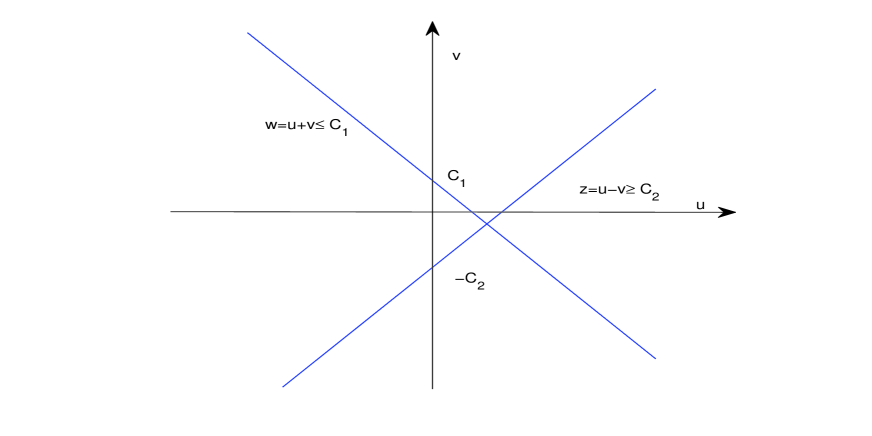
Figure 1. Graphs of level sets of $w$ and $z$

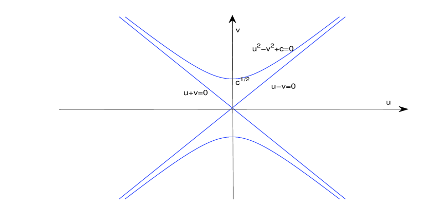
Figure 2. Graphs of $\varphi_{1}(u,v)=0,\varphi_{2}(u,v)=0$ when $\alpha=-1$

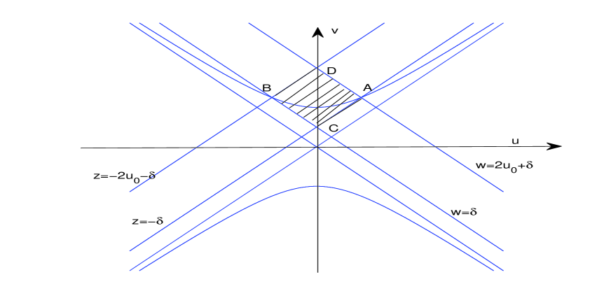
Figure 3. Invariant region when $\alpha=-1$

To obtain the invariant region we need to sketch the graphs of

$$\varphi_{1}(u,v)=0,\,\varphi_{2}(u,v)=0$$

in the $u-v$ plane in Figure 2. Now let us find the invariant region in the upper half-plane. We draw a straight line parallel to $u-v=0$ passing through the point

$$C=(0,\delta)$$

with $0<\delta<\sqrt{c}$ intersecting the hyperbola at the point

$$A=(u_{0},u_{0}+\delta),$$

and similarly, we get the point

$$B=(-u_{0},u_{0}+\delta),$$

where

$$u_{0}=u_{0}(-1)=\frac{c-\delta^{2}}{2\delta}.$$ (3.9)

We then draw a straight line perpendicular to $u-v=0$ passing through the point $A$ and another straight line perpendicular to $u+v=0$ through $B$. Then the two lines intersect the $v-$axis at the same point

$$D=\left(0,\frac{c-\delta^{2}}{2\delta}\right);$$

see Figure 3. We see that the square $ACBD$ in Figure 3 is an invariant region. Therefore we get the $L^{\infty}$ estimate of $(u,v)$, that is,

$$-\frac{c-\delta^{2}}{2\delta}\leq u\leq\frac{c-\delta^{2}}{2\delta},\quad\delta\leq v\leq\frac{c}{\delta}.$$ (3.10)

When $\alpha<-1$, the graphs of $\varphi_{1}(u,v)=0,\,\varphi_{2}(u,v)=0$ in the $u-v$ plane look like the curves marked with $1$ and $2$ respectively in Figure 4. Similarly to the case $\alpha=-1$, we draw a straight line parallel to $u-v=0$ passing through the point

$$C=(0,\delta)$$

with $0<\delta<\sqrt{-2c\alpha-c}$ intersecting the curve $\varphi_{1}(u,v)=0$ at the point

$$A=(u_{0},u_{0}+\delta).$$

Then we draw a straight line parallel to $u+v=0$ passing through the point $C=(0,\delta)$ intersecting the curve $\varphi_{2}(u,v)=0$ at the point

$$B=(-u_{0},u_{0}+\delta).$$

Moreover, we draw a straight line perpendicular to $u-v=0$ passing through point $A$ and another straight line perpendicular to $u+v=0$ passing through point $B$. Then the two lines intersect the $v-$axis at the same point

$$D=(0,2u_{0}+\delta).$$

Thus, the square $ACBD$ in Figure 5 is an invariant region, and now the $L^{\infty}$ estimate of $(u,v)$ is

$$-u_{0}\leq u\leq u_{0},\quad\delta\leq v\leq 2u_{0}+\delta,$$ (3.11)

where

$$0<\delta<\sqrt{-2c\alpha-c},$$

$$u_{0}=u_{0}(\alpha)=-\frac{c\alpha+2\delta^{2}-\sqrt{c^{2}\alpha^{2}-4c\alpha\delta^{2}-4c\delta^{2}}}{4\delta}.$$ (3.12)

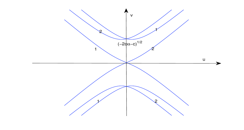
Figure 4. Graphs of $\varphi_{1}(u,v)=0,\varphi_{2}(u,v)=0$ when $\alpha<-1$.

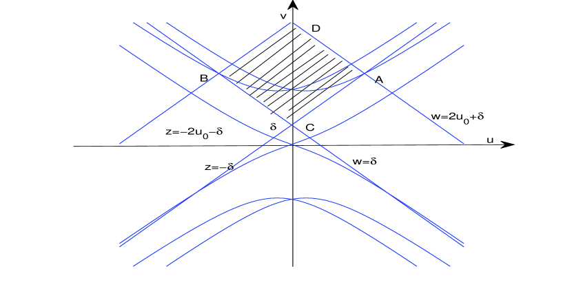
Figure 5. Invariant region when $\alpha<-1$

Example 3.1.

For the following special catenoid type surfaces with

$$E(y)=\left(c\cosh\left(\frac{y}{c}\right)\right)^{\frac{2}{\beta^{2}-1}},\quad G(y)=\frac{1}{c^{2}(\beta^{2}-1)^{2}}E(y),$$

and

$$K(y)=-c^{2}(\beta^{2}-1)E(y)^{-\beta^{2}},$$

where $c\neq 0,\,\beta\geq\sqrt{2}$ are constants, one has $E(y)^{\prime}>0$ whenever $y>0$, and $E(y)^{\prime}<0$ whenever $y<0$. All the conditions (3.4) and (3.8) for the above invariant region are satisfied when $y<0$. If we take $\Omega=\{(x,y):x\in\mathbb{R},-y_{0}\leq y\leq 0\}$, where $y_{0}>0$ is arbitrary, then in $\Omega$ the equations (2.19) are parabolic for $y-$time like. Therefore, when the initial value $(u(x,-y_{0}),v(x,-y_{0}))$ is in the square $ACBD$, the parabolic maximum/minimum principle ensures that the square $ACBD$ is an invariant region, which yields the $L^{\infty}$ estimate. We notice that the surface is just the classical catenoid when $\beta=\sqrt{2}$. Indeed, for the special catenoid type metric, the surface is given by the following function:

$$\mathbf{r}(x,y)=(r_{1}(x,y),r_{2}(x,y),r_{3}(x,y)),$$

with

$$r_{1}(x,y)=\left(c\cosh\left(\frac{y}{c}\right)\right)^{\frac{1}{\beta^{2}-1}}\sin(x),$$

$$r_{2}(x,y)=\left(c\cosh\left(\frac{y}{c}\right)\right)^{\frac{1}{\beta^{2}-1}}\cos(x),$$

$$r_{3}(x,y)=\int^{y}\frac{1}{(\beta^{2}-1)^{2}}\left(c\cosh\left(\frac{t}{c}\right)\right)^{\frac{4-2\beta^{2}}{\beta^{2}-1}}dt.$$

3.2. Helicoid type surfaces: $E(y)=B(y)^{2},F=0,G(y)=1$

For the surfaces with the metric of the form:

$$E(y)=B(y)^{2},\quad F=0,\quad G(y)=1,\quad B(y)>0,$$ (3.13)

we can also calculate that

$$\Gamma^{2}_{22}=0,\quad\Gamma^{2}_{12}=0,\quad\Gamma^{2}_{11}=\frac{-E^{\prime}}{2E},\quad\Gamma^{1}_{22}=0,\quad\Gamma^{1}_{12}=\frac{E^{\prime}}{2E},\quad\Gamma^{1}_{11}=0.$$

and

$$\begin{split}\tilde{\Gamma}^{2}_{22}=\frac{\gamma^{\prime}}{\gamma},\qquad\tilde{\Gamma}^{2}_{12}=0,\qquad\tilde{\Gamma}^{2}_{11}=\frac{-E^{\prime}}{2},\\ \tilde{\Gamma}^{1}_{22}=0,\qquad\tilde{\Gamma}^{1}_{12}=\frac{E^{\prime}}{2E}+\frac{\gamma^{\prime}}{2\gamma},\qquad\tilde{\Gamma}^{1}_{11}=0.\end{split}$$

Then

$$\begin{split}&f(u,v)=-\frac{E^{\prime}}{E}u-\frac{E^{\prime}}{2}(u^{2}-v^{2})u,\\ &g(u,v)=\frac{\gamma^{\prime}}{\gamma}v-\frac{E^{\prime}}{2}(u^{2}-v^{2})v.\end{split}$$

Assuming

$$\frac{\gamma^{\prime}}{\gamma}=a\frac{B^{\prime}}{B},$$

and using $E(y)=B(y)^{2}$ and (2.3), we have

$$a\frac{E^{\prime}}{E}=\frac{K^{\prime}}{K},$$

that is,

$$K(y)=-k_{0}E(y)^{a},$$ (3.14)

with some constant $k_{0}>0$. Thus,

$$\begin{split}&f(u,v)=-\frac{2B^{\prime}}{B}u-BB^{\prime}(u^{2}-v^{2})u,\\ &g(u,v)=a\frac{B^{\prime}}{B}v-BB^{\prime}(u^{2}-v^{2})v,\end{split}$$

and

$$\begin{split}&f(u,v)+g(u,v)=-\frac{2B^{\prime}}{B}u+a\frac{B^{\prime}}{B}v-BB^{\prime}(u^{2}-v^{2})(u+v),\\ &f(u,v)-g(u,v)=-\frac{2B^{\prime}}{B}u-a\frac{B^{\prime}}{B}v-BB^{\prime}(u^{2}-v^{2})(u-v).\end{split}$$

Now set

$$\begin{split}\tilde{u}=Bu,\quad&\tilde{v}=Bv,\\ \tilde{w}=Bu+Bv=\tilde{u}+\tilde{v},\quad&\tilde{z}=Bu-Bv=\tilde{u}-\tilde{v}.\end{split}$$ (3.15)

Since $B$ depends only on $y$, we have

$$\begin{split}&\tilde{w}_{y}+\lambda_{1}\tilde{w}_{x}=\varepsilon\tilde{w}_{xx}-\frac{2\varepsilon v_{x}\tilde{w}_{x}}{v}+(f(u,v)+g(u,v))B+\frac{B^{\prime}}{B}\tilde{w},\\ &\tilde{z}_{y}+\lambda_{2}\tilde{z}_{x}=\varepsilon\tilde{z}_{xx}-\frac{2\varepsilon v_{x}\tilde{z}_{x}}{v}+(f(u,v)-g(u,v))B+\frac{B^{\prime}}{B}\tilde{z}.\end{split}$$ (3.16)

Note that

$$f(u,v)+g(u,v)=-\frac{B^{\prime}}{B^{2}}\left(2Bu-aBv+((Bu)^{2}-(Bv)^{2})(Bu+Bv)\right),$$

then

$$\begin{split}R_{1}(u,v):=&(f(u,v)+g(u,v))B+\frac{B^{\prime}}{B}\tilde{w}\\ =&-\frac{B^{\prime}}{B}\left(2\tilde{u}-a\tilde{v}+(\tilde{u}^{2}-\tilde{v}^{2})(\tilde{u}+\tilde{v})\right)+\frac{B^{\prime}}{B}(\tilde{u}+\tilde{v})\\ =&-\frac{B^{\prime}}{B}\left(\tilde{u}-(a+1)\tilde{v}+(\tilde{u}^{2}-\tilde{v}^{2})(\tilde{u}+\tilde{v})\right),\end{split}$$

and similarly,

$$\begin{split}R_{2}(u,v):=&(f(u,v)-g(u,v))B+\frac{B^{\prime}}{B}\tilde{z}\\ =&-\frac{B^{\prime}}{B}\left(\tilde{u}+(a+1)\tilde{v}+(\tilde{u}^{2}-\tilde{v}^{2})(\tilde{u}-\tilde{v})\right).\end{split}$$

Since $B(y)>0$ is given, it remains to find the invariant region of $\tilde{w},\tilde{z}$. As in the catenoid case in Subsection 3.1, we need to analyze the signs of $R_{1}$ and $R_{2}$. If we assume

$$B^{\prime}<0,$$

or equivalently, from $E=B^{2}$,

$$E^{\prime}<0,$$ (3.17)

and set

$$\begin{split}&\psi_{1}(\tilde{u},\tilde{v}):=\tilde{u}-(a+1)\tilde{v}+(\tilde{u}^{2}-\tilde{v}^{2})(\tilde{u}+\tilde{v}),\\ &\psi_{2}(\tilde{u},\tilde{v}):=\tilde{u}+(a+1)\tilde{v}+(\tilde{u}^{2}-\tilde{v}^{2})(\tilde{u}-\tilde{v}),\end{split}$$

then the signs of $R_{1}(\tilde{u},\tilde{v}),R_{2}(\tilde{u},\tilde{v})$ depend on the signs of $\psi_{1}(\tilde{u},\tilde{v}),\psi_{2}(\tilde{u},\tilde{v})$ respectively. Now we end up with a situation similar to the catenoid case in Subsection 3.1 with $c=1,\,a=2\alpha$, and the corresponding $\varphi_{i}$ ($i=1,2$) in Subsection 3.1 are

$$\varphi_{1}(\tilde{u},\tilde{v})=\psi_{1}(\tilde{u},\tilde{v}),\quad\varphi_{2}(\tilde{u},\tilde{v})=\psi_{2}(\tilde{u},\tilde{v}).$$

We can find the invariant regions just as in catenoid case in Subsection 3.1. Indeed, the invariant region of $(\tilde{u},\tilde{v})$ looks like the same as the invariant region $ACBD$ in Figure 3 when $a=-2$ if we replace the $u-v$ plane by the $\tilde{u}-\tilde{v}$ plane and $u_{0}$ by $\tilde{u}_{0}=\tilde{u}_{0}(-2)$ defined below; and looks like the same as the invariant region $ACBD$ in Figure 5 when $a<-2$ in the $\tilde{u}-\tilde{v}$ plane, and thus we omit the sketch of the invariant regions. From the invariant region, when $a=-2$,

$$-\frac{1-\delta^{2}}{2\delta}\leq\tilde{u}\leq\frac{1-\delta^{2}}{2\delta},\qquad\delta\leq\tilde{v}\leq\frac{1}{\delta};$$ (3.18)

and when $a<-2$,

$$-\tilde{u}_{0}\leq\tilde{u}\leq\tilde{u}_{0},\qquad\delta\leq\tilde{v}\leq 2\tilde{u}_{0}+\delta,$$ (3.19)

where

$$0<\delta<\sqrt{-a-1},$$

$$\tilde{u}_{0}=\tilde{u}_{0}(a)=\frac{-a-4\delta^{2}+\sqrt{a^{2}-8a\delta^{2}-16\delta^{2}}}{8\delta}.$$ (3.20)

Note that $0<B(y)\in C^{1,1}(\Omega)$, we can easily obtain the $L^{\infty}$ boundedness of $u,v$.

Example 3.2.

For the helicoid surface with

$$E(y)=c^{2}+y^{2},\quad F(y)\equiv 0,\quad G(y)\equiv 1,\quad K(y)=-\frac{c^{2}}{(c^{2}+y^{2})^{2}},$$

where $c\neq 0$, we see that

$$B(y)=\sqrt{c^{2}+y^{2}},$$

and $B(y)^{\prime}>0$ for $y>0$, and $B(y)^{\prime}<0$ for $y<0$. If we take

$$\Omega=\{(x,y):x\in\mathbb{R},-y_{0}\leq y\leq 0\},$$

where $y_{0}>0$ is an arbitrary constant, then in $\Omega$, the equations in (2.19) are parabolic for $y-$time like. Therefore, when the initial value $(u(x,-y_{0}),v(x,-y_{0}))$ is in the square $ACBD$, we have the invariant region for the solutions. We note that the function for the helicoid in $\mathbb{R}^{3}$ is $\mathbf{r}(x,y)=(y\sin x,y\cos x,cx).$

Remark 3.1.

We can see from Figures 3 and 5 that the $L^{\infty}$ estimates also hold for $v<0$ since we can also find the invariant regions in the lower half-plane of $u-v$, which are symmetric with the invariant regions in the upper half-plane around the $u$ axis.

4. $H^{-1}$ Compactness

In this section we shall prove the $H^{-1}_{loc}$ compactness of the approximate viscous solutions.

For the strictly convex entropy

$$\eta=\frac{\tilde{M}^{2}+1}{\tilde{L}},$$

and entropy flux

$$q=\frac{-\tilde{M}^{3}+\tilde{M}}{\tilde{L}^{2}},$$

from the parabolic equations (2.8), one has

$$\begin{split}\eta_{y}+q_{x}&=\varepsilon\eta_{xx}+\Pi(\tilde{L},\tilde{M})-2\varepsilon\left(\frac{\tilde{M}^{2}+1}{\tilde{L}^{3}}\tilde{L}_{x}^{2}-2\frac{\tilde{M}}{\tilde{L}^{2}}\tilde{L}_{x}\tilde{M}_{x}+\frac{\tilde{M}_{x}^{2}}{\tilde{L}}\right)\\ &=\varepsilon\eta_{xx}+\Pi(\tilde{L},\tilde{M})-2\varepsilon\left(\frac{\tilde{L}_{x}^{2}}{\tilde{L}^{3}}+\frac{1}{\tilde{L}}\left(\frac{\tilde{M}}{\tilde{L}}\tilde{L}_{x}-\tilde{M}_{x}\right)^{2}\right),\end{split}$$ (4.1)

where

$$\begin{split}\Pi(\tilde{L},\tilde{M})=&\frac{\tilde{M}^{2}+1}{\tilde{L}^{2}}\left(\tilde{\Gamma}^{2}_{22}\tilde{L}-2\tilde{\Gamma}^{2}_{12}\tilde{M}+\tilde{\Gamma}^{2}_{11}\tilde{N}\right)\\ &+\frac{2\tilde{M}}{\tilde{L}}\left(\tilde{\Gamma}^{1}_{22}\tilde{L}-2\tilde{\Gamma}^{1}_{12}\tilde{M}+\tilde{\Gamma}^{1}_{11}\tilde{N}\right).\end{split}$$

From

$$\tilde{L}=\frac{1}{v},\quad\tilde{M}=-\frac{u}{v},$$

we have

$$\tilde{L}_{x}=-\frac{v_{x}}{v^{2}},\quad\tilde{M}_{x}=\frac{uv_{x}}{v^{2}}-\frac{u_{x}}{v},$$

and thus

$$\eta_{y}+q_{x}=\varepsilon\eta_{xx}+\Pi(\tilde{L},\tilde{M})-2\varepsilon\left(\frac{v_{x}^{2}}{v}+\frac{u_{x}^{2}}{v}\right).$$ (4.2)

Due to the $L^{\infty}$ uniform estimates for $u$ and $v$ in Subsections 3.1 and 3.2, we have

$$0<b_{1}(\delta)\leq\tilde{L}\leq b_{2}(\delta),\quad|\tilde{M}|\leq b_{3}(\delta),$$ (4.3)

uniformly in $\varepsilon$ in $\Omega$, where $b_{1}(\delta)$, $b_{2}(\delta)$ and $b_{3}(\delta)$ are positive constants depending on $\delta>0$. Therefore $\Pi(\tilde{L},\tilde{M})$ is also uniformly bounded in $\varepsilon$. Let

$$\Omega=\{(x,y):x\in\mathbb{R},-y_{0}\leq y\leq 0\},$$

where $y_{0}>0$ is arbitrary. Choose the test function $\phi\in C^{\infty}_{c}(\Omega)$ satisfying $\phi|_{K}\equiv 1$, $0\leq\phi\leq 1$, where $K$ is a compact set and $K\subset S=\text{supp }\phi$. From $\eqref{10b}$, we have

$$\begin{split}&\int_{-\infty}^{\infty}\int_{-y_{0}}^{0}2\varepsilon\left(\frac{v_{x}^{2}}{v}+\frac{u_{x}^{2}}{v}\right)\phi dydx\\ &\leq\int_{-\infty}^{\infty}\int_{-y_{0}}^{0}\left(\varepsilon\eta_{xx}-\eta_{y}-q_{x}+\Pi(\tilde{L},\tilde{M})\right)\phi dydx\\ &=\int_{-\infty}^{\infty}\int_{-y_{0}}^{0}\left(\varepsilon\eta\phi_{xx}+\eta\phi_{y}+q\phi_{x}+\Pi(\tilde{L},\tilde{M})\phi\right)dydx\\ &\leq M(\phi)\end{split}$$ (4.4)

for some positive constant $M(\phi)$ uniform in $\varepsilon\in(0,1)$. Since $v$ is uniformly bounded from below with positive lower bound, $\varepsilon v_{x}^{2},\,\varepsilon u_{x}^{2}$ are bounded in $L^{1}_{loc}(\Omega)$. Since $u$ is uniformly bounded and $v$ has uniform positive lower bound, one has

$$\varepsilon\tilde{L}_{x}^{2}=\varepsilon\frac{v_{x}^{2}}{v^{4}}\leq C\varepsilon v_{x}^{2},\quad\varepsilon\tilde{M}_{x}^{2}=\varepsilon\left(\frac{uv_{x}}{v^{2}}-\frac{u_{x}}{v}\right)^{2}\leq C\varepsilon(v_{x}^{2}+u_{x}^{2}),$$

for some positive constant $C$ uniform in $\varepsilon$, then we see that $\varepsilon\tilde{L}_{x}^{2}$ and $\varepsilon\tilde{M}_{x}^{2}$ are uniformly bounded in $L^{1}_{loc}(\Omega)$. Noting that

$$\varepsilon\tilde{L}_{xx}=\sqrt{\varepsilon}(\sqrt{\varepsilon}\tilde{L}_{x})_{x},$$

and for arbitrary $\phi\in C_{c}^{\infty}(\Omega)$,

$$\begin{split}&\int_{-\infty}^{\infty}\int_{-y_{0}}^{0}\varepsilon\tilde{L}_{xx}\phi dydx=\int_{-\infty}^{\infty}\int_{-y_{0}}^{0}\varepsilon\tilde{L}_{x}\phi_{x}dydx\\ &\leq\sqrt{\varepsilon}\left(\int_{\text{supp }\phi}\varepsilon\tilde{L}_{x}^{2}dydx\right)^{\frac{1}{2}}\left(\int_{\Omega}(\phi_{x})^{2}dydx\right)^{\frac{1}{2}}\\ &\leq C\sqrt{\varepsilon}\rightarrow 0\text{ as }\varepsilon\rightarrow 0,\end{split}$$ (4.5)

we see that $\varepsilon\tilde{L}_{xx}$ is compact in $H^{-1}_{loc}(\Omega)$. From (2.8), we have

$$\tilde{M}_{x}-\tilde{L}_{y}=\tilde{\Gamma}^{2}_{22}\tilde{L}-2\tilde{\Gamma}^{2}_{12}\tilde{M}+\tilde{\Gamma}^{2}_{11}\tilde{N}-\varepsilon\tilde{L}_{xx}.$$ (4.6)

Since $\tilde{\Gamma}^{2}_{22}\tilde{L}-2\tilde{\Gamma}^{2}_{12}\tilde{M}+\tilde{\Gamma}^{2}_{11}\tilde{N}$ is uniformly bounded in $\Omega$, it is uniformly bounded in $L^{1}_{loc}(\Omega)$ and compact in $W^{-1,p}_{loc}(\Omega)$ with some $1<p<2$ by the imbedding theorem and the Schauder theorem. Therefore $\tilde{M}_{x}-\tilde{L}_{y}$ is compact in $W^{-1,p}_{loc}(\Omega)$. Moreover, we see that $\tilde{M}_{x}-\tilde{L}_{y}$ is uniformly bounded in $W^{-1,\infty}_{loc}(\Omega)$ since $\tilde{M}$ and $\tilde{L}$ are uniformly bounded. Finally, by Lemma 4.1 below, we conclude that $\tilde{M}_{x}-\tilde{L}_{y}$ is compact in $H^{-1}_{loc}(\Omega)$. Similarly, $\tilde{N}_{x}-\tilde{M}_{y}$ is also compact in $H^{-1}_{loc}(\Omega)$. Since $\gamma$ is $C^{1}$, we see that $M_{x}-L_{y}$ and $N_{x}-M_{y}$ are also compact in $H^{-1}_{loc}(\Omega).$

We record the following useful lemma (see [7, 48]) here:

Lemma 4.1.

Let $\Omega\in\mathbb{R}^{n}$ be a open set, then (compact set of $W^{-1,q}_{loc}(\Omega)$ ) $\bigcap$ (bounded set of $W_{loc}^{-1,r}(\Omega)$ ) $\subset$ (compact set of $H^{-1}_{loc}(\Omega)$). where $q$ and $r$ are constants, $1<q\leq 2<r.$

5. Main Theorems and Proofs

In this section, we shall state our main results and also give the proof.

In the previous sections, we have established the $L^{\infty}$ uniform estimate and $H_{loc}^{-1}$ compactness of the viscous approximate solutions to (2.8) for some special metrics of the form

$$ds^{2}=Edx^{2}+Gdy^{2}.$$

The corresponding Gauss curvature $K(x,y)=K$ has the following form (see [27]):

$$K=\frac{1}{4EG}\left(\frac{E_{y}^{2}+E_{x}G_{x}}{E}+\frac{G_{x}^{2}+E_{y}G_{y}}{G_{y}}-2(E_{yy}+G_{xx})\right).$$ (5.1)

To prove the existence of isometric immersion, first let us recall the following compensated compactness framework in Theorem 4.1 of [8]:

Lemma 5.1.

Let a sequence of functions $(L^{\varepsilon},M^{\varepsilon},N^{\varepsilon})(x,y)$, defined on an open subset $\Omega\subset\mathbb{R}^{2}$, satisfy the following framework:

• $(L^{\varepsilon},M^{\varepsilon},N^{\varepsilon})(x,y)$ is uniformly bounded almost everywhere in $\Omega\subset\mathbb{R}^{2}$ with respect to $\varepsilon$;

• $M^{\varepsilon}_{x}-L^{\varepsilon}_{y}$ and $N^{\varepsilon}_{x}-M^{\varepsilon}_{y}$ are compact in $H^{-1}_{loc}(\Omega)$;

• There exist $o_{j}^{\varepsilon}(1)$, $j=1,2,3$, with $o_{j}^{\varepsilon}(1)\rightarrow 0$ in the sense of distributions as $\varepsilon\rightarrow 0$ such that

  $$\begin{split}&M_{x}^{\varepsilon}-L_{y}^{\varepsilon}=\Gamma^{2}_{22}L^{\varepsilon}-2\Gamma^{2}_{12}M^{\varepsilon}+\Gamma^{2}_{11}N^{\varepsilon}+o_{1}^{\varepsilon}(1),\\ &N_{x}^{\varepsilon}-M_{y}^{\varepsilon}=-\Gamma^{1}_{22}L^{\varepsilon}+2\Gamma^{1}_{12}M^{\varepsilon}-\Gamma^{1}_{11}N^{\varepsilon}+o_{2}^{\varepsilon}(1),\\ \end{split}$$ (5.2)

  and

  $$L^{\varepsilon}N^{\varepsilon}-(M^{\varepsilon})^{2}=K+o_{3}^{\varepsilon}(1).$$ (5.3)

Then there exists a subsequence (still labeled) $(L^{\varepsilon},M^{\varepsilon},N^{\varepsilon})$ converging weak-star in $L^{\infty}$ to $(L,M,N)(x,y)$ as $\varepsilon\rightarrow 0$ such that

• $(L,M,N)$ is also bounded in $\Omega\subset\mathbb{R}^{2}$;

• the Gauss equation (5.3) is weakly continuous with respect to the subsequence $(L^{\varepsilon},M^{\varepsilon},N^{\varepsilon})$ converging weak-star in $L^{\infty}$ to $(L,M,N)(x,y)$ as $\varepsilon\rightarrow 0$;

• The Codazzi equations (5.2) as $\varepsilon\to 0$ hold for $(L,M,N)$ in the sense of distribution.

We now present the results on the existence of isometric immersion of surfaces with the two types of metrics studied in Section 3.

Definition 5.1.

A Riemannian metric on a two-dimensional manifold is called a catenoid metric if it is of the form

$$ds^{2}=E(y)dx^{2}+cE(y)dy^{2},$$

with

$$c>0,\quad E(y)>0,\quad E(y)^{\prime}<0\text{ for }y<0,$$

and the corresponding Gauss curvature is of the form

$$K(y)=-k_{0}E(y)^{-\beta^{2}}$$

with constants $k_{0}>0$ and $\beta\geq\sqrt{2}$.

From the Definition 5.1 and the formula in (5.1), we see that $E(y)$ satisfies the following ordinary differential equation:

$$(E(y)^{\prime})^{2}-EE(y)^{\prime\prime}=-2k_{0}E(y)^{2-\beta^{2}}.$$ (5.4)

We can solve it through the following process utilizing the method of [42]. Set

$$E(y)=e^{w(y)},$$

then

$$E(y)^{\prime}=e^{w(y)}w(y)^{\prime},\quad E(y)^{\prime\prime}=e^{w(y)}\left((w(y)^{\prime})^{2}+w(y)^{\prime\prime}\right),$$

and (5.4) becomes

$$w(y)^{\prime\prime}=2k_{0}e^{-\beta^{2}w(y)}.$$ (5.5)

Let $f(w(y))=w(y)^{\prime}.$ After differentiating respect to $y$, we get

$$f(w)^{\prime}w(y)^{\prime}=w(y)^{\prime\prime},$$

i.e.,

$$f(w)f(w)^{\prime}=2k_{0}e^{-\beta^{2}w},$$

therefore, noting that $E^{\prime}<0$ implies $w^{\prime}<0$,

$$f(w)=\frac{dw}{dy}=-\sqrt{C_{1}-\frac{4k_{0}}{\beta^{2}}e^{-\beta^{2}w}}.$$

Then one has

$$y=C_{2}-\int\frac{dw}{\sqrt{C_{1}-\frac{4k_{0}}{\beta^{2}}e^{-\beta^{2}w}}},$$

Denote the right side of the above equation by $h(w)$, then $w(y)=h^{-1}(y)$ and $E(y)=e^{h^{-1}(y)}$, where $h^{-1}(y)$ is the inverse function of $h(w)$, $C_{1}$ and $C_{2}$ depend on the the value of $w(0)$ and $w(0)^{\prime}$. Then the catenoid metric is of the form:

$$ds^{2}=e^{h^{-1}(y)}dx^{2}+ce^{h^{-1}(y)}dy^{2}.$$ (5.6)

We note that the special catenoid type metric given in Example 3.1:

$$E(y)=\left(c\cosh\left(\frac{y}{c}\right)\right)^{\frac{2}{\beta^{2}-1}},\quad G(y)=\frac{1}{c^{2}(\beta^{2}-1)^{2}}E(y),$$

with $K(y)=-c^{2}(\beta^{2}-1)E(y)^{-\beta^{2}}$ is a catenoid metric in the sense of Definition 5.1.

Definition 5.2.

A Riemannian metric on a two-dimensional manifold is called a helicoid metric if it is of the form

$$ds^{2}=E(y)dx^{2}+dy^{2},$$

with

$$E(y)>0,\quad E(y)^{\prime}<0\text{ for }y<0,$$

and the corresponding Gauss curvature is of the form

$$K(y)=-k_{0}E(y)^{a}$$

with constants $k_{0}>0$ and $a\leq-2$.

From Definition 5.2 and the formula (5.1), $E(y)$ satisfies the following ordinary differential equation:

$$(E(y)^{\prime})^{2}-2EE(y)^{\prime\prime}=-4k_{0}E(y)^{2+a}.$$ (5.7)

Set

$$E(y)=w(y)^{2},$$

then (5.7) becomes

$$w(y)^{\prime\prime}=k_{0}w(y)^{2a+1}.$$

Letting $g(w(y))=w(y)^{\prime}$, and differentiating respect to $y$, one has

$$w(y)^{\prime\prime}=u(w)^{\prime}w(y)^{\prime},$$

i.e.,

$$g(w)^{\prime}g(w)=k_{0}w^{2a+1}.$$

Thus

$$g(w)=\frac{dw}{dy}=-\sqrt{C_{1}+\frac{k_{0}}{a+1}w^{2a+2}}.$$

Then

$$y=C_{2}-\int\frac{dw}{\sqrt{{C_{1}+\frac{k_{0}}{a+1}}w^{2a+2}}}.$$

Denote the right side of the above equation by $h(w)$, then $w(y)=h^{-1}(y),$ and $E(y)=(h^{-1}(y))^{2}.$ Therefore, the helicoid metric is

$$ds^{2}=(h^{-1}(y))^{2}dx^{2}+dy^{2},$$

where $h^{-1}(y)$ is the inverse function of

$$h(w)=C_{2}-\int\frac{dw}{\sqrt{C_{1}+\frac{k_{0}}{a+1}w^{2a+2}}}.$$

Similar to the catenoid metric, $C_{1}$ and $C_{2}$ depend on the value of $w(0)$ and $w(0)^{\prime}$. As an example, the helicoid surface with

$$E(y)=c^{2}+y^{2},\quad K(y)=-\frac{c^{2}}{(c^{2}+y^{2})^{2}}$$

is a two-dimensional Riemannian manifold with the helicoid metric in the sense of Definition 5.2.

Now we prove the existence of $C^{1,1}$ isometric immersion of surfaces with the above two types of metrics into $\mathbb{R}^{3}$ by using Lemma 5.1.

Theorem 5.1.

For any given $y_{0}>0$, let the initial data

$$(u,v)|_{y=-y_{0}}=(\bar{u}_{0}(x),\bar{v}_{0}(x)):=(u(x,-y_{0}),v(x,-y_{0}))$$ (5.8)

satisfy the following conditions:

$$\bar{u}_{0}+\bar{v}_{0}\text{ and }\bar{u}_{0}-\bar{v}_{0}\text{ are bounded},$$

and

$$\inf_{x\in\mathbb{R}}\left(\bar{u}_{0}+\bar{v}_{0}\right)>0,\quad\sup_{x\in\mathbb{R}}\left(\bar{u}_{0}-\bar{v}_{0}\right)<0.$$

Then, for the catenoid metric in the sense of Definition 5.1, the Gauss-Codazzi system (2.1) has a weak solution in $\Omega=\{(x,y):x\in\mathbb{R},-y_{0}\leq y\leq 0\}$ with the initial data (5.8).

Remark 5.1.

For the initial data $(\bar{u}_{0}(x),\bar{v}_{0}(x))$ satisfying the conditions in Theorem 5.1, there exists a constant $\delta>0$, such that

$$\begin{split}(\bar{u}_{0}(x),\bar{v}_{0}(x))\in ACBD:=\{(u,v):\;\;&\delta\leq w=u+v\leq 2u_{0}+\delta,\\ &-(2u_{0}+\delta)\leq z=u-v\leq-\delta\},\end{split}$$

for the catenoid type metrics, where $u_{0}$ is defined in (3.12). That is, $(\bar{u}_{0}(x),\bar{v}_{0}(x))$ lies in the invariant region $ACBD$ sketched in Figure 3 or Figure 5, i.e., $\bar{u}_{0}(x)$ is bounded, and $\bar{v}_{0}(x)$ has positive lower bound and upper bound.

Proof.

First for the initial data (5.8), the corresponding initial data for $\tilde{L},\tilde{M},\tilde{N}$ is

$$\tilde{L}_{0}(x)=\frac{1}{\bar{v}_{0}(x)},\quad\tilde{M}_{0}(x)=\frac{-\bar{u}_{0}(x)}{\bar{v}_{0}(x)},\quad\tilde{N}_{0}(x)=\frac{\bar{u}_{0}(x)^{2}-\bar{v}_{0}(x)^{2}}{\bar{v}_{0}(x)}.$$

We use system (2.19) to obtain the approximate viscous solutions and their $L^{\infty}$ estimate, and then use (2.8) to obtain the $H^{-1}_{loc}$ compactness.

Step 1. We mollify the initial data (5.8) as

$$\bar{u}_{0}^{\varepsilon}(x)=\bar{u}_{0}(x)\ast j^{\varepsilon},\quad\bar{v}_{0}^{\varepsilon}(x)=\bar{v}_{0}(x)\ast j^{\varepsilon},$$

where $j^{\varepsilon}$ is the standard mollifier and $\ast$ is for the convolution. From the above Remark 5.1, there exists a $\delta>0$, such that,

$$|\bar{u}_{0}^{\varepsilon}(x)|\leq M(\delta),\quad 0<\delta\leq\bar{v}_{0}^{\varepsilon}(x)\leq M(\delta),$$

where $M(\delta)$ is positive constant depending on $\delta$, and

$$(\bar{u}_{0}^{\varepsilon}(x),\bar{v}_{0}^{\varepsilon}(x))\rightarrow(\bar{u}_{0}(x),\bar{v}_{0}(x))\text{ as }\varepsilon\rightarrow 0,\qquad a.e.$$

Step 2. The local existence of (2.8) can be obtained by the standard theory, hence we have the local existence of (2.19). From Section 3, we have the $L^{\infty}$ estimate for the approximate solution of (2.19), then we can obtain the global existence of the approximate solution as follows. We observe that the first equation of (2.19) is of the divergence form, thus the estimate of $u_{x}$ can be handled in the standard way. However, the second equation of (2.19) is not in divergence form. By differentiation of the second equation with respect to $x$, we get

$$(v_{x})_{y}+(uv_{x}-vu_{x})_{x}=g(u,v)_{x}+\varepsilon(v_{x})_{xx}-\Big{(}\frac{2\varepsilon v_{x}^{2}}{v}\Big{)}_{x},$$

where we omit $\varepsilon$ and still use $u(x,y),v(x,y)$ for the approximate solution of (2.19). Let $G(x,y)$ is the heat kernel of $h_{y}=\varepsilon h_{xx}$, then we can solve the above equation as the following:

$$\begin{split}v_{x}=&\int_{-\infty}^{\infty}G(x-\xi,y)\bar{v}_{0x}^{\varepsilon}(\xi)d\xi\\ &+\int_{-y_{0}}^{0}\int_{-\infty}^{\infty}\left(g(u,v)_{x}-(uv_{x}-vu_{x})_{x}+\Big{(}\frac{2\varepsilon v_{x}^{2}}{v}\Big{)}_{x}\right)G(x-\xi,y-\eta)d\xi d\eta\\ =&\int_{-\infty}^{\infty}G(x-\xi,y)\bar{v}_{0x}^{\varepsilon}(\xi)d\xi\\ &+\int_{-y_{0}}^{0}\int_{-\infty}^{\infty}\left(-g(u,v)+(uv_{x}-vu_{x})+\frac{2\varepsilon v_{x}^{2}}{v}\right)G(x-\xi,y-\eta)_{x}d\xi d\eta.\end{split}$$

Therefore

$$\begin{split}&||v_{x}||_{C^{0}}\leq\int_{-\infty}^{\infty}G(x-\xi,y)|\bar{v}_{0x}^{\varepsilon}(\xi)|d\xi\\ &\qquad\qquad+\int_{-y_{0}}^{0}\int_{-\infty}^{\infty}\left(|g(u,v)|+|(uv_{x}-vu_{x})|+\left|\frac{2\varepsilon v_{x}^{2}}{v}\right|\right)G(x-\xi,y-\eta)_{x}|d\xi d\eta\\ &\leq||\bar{v}_{0x}^{\varepsilon}||_{C^{0}}+M(\delta)(||u_{x}||_{C^{0}}|+||v_{x}||_{C^{0}}+\varepsilon||v_{x}||_{C^{0}})\int_{-y_{0}}^{0}\int_{-\infty}^{\infty}|G(x-\xi,y-\eta)_{x}|d\xi d\eta,\end{split}$$

where $||\cdot||_{C^{0}}$ stands for the norm of continuous functions. The above process yields the $C^{0}$ estimate of $v_{x}$. Similarly, we can estimate $C^{k}$ (for any integer $k\geq 1$) norms of $u(x,y),v(x,y)$, which can be bounded by the $C^{k}$ norms of $\bar{u}_{0}^{\varepsilon}$ and $\bar{v}_{0}^{\varepsilon}$. Thus, we obtain the global existence of smooth solutions to the system (2.19).

Step 3. In Section 3 we have proved $L^{\infty}$ boundness of $\tilde{L},\tilde{M},\tilde{N}$, and then $L,M,N$ is in $L^{\infty}$ for $\gamma\in C^{1}$. By the reverse process of Section 2, we can reformulate the equations (2.19) of $u$ and $v$ as the equations (2.8). Therefore, as in Section 4 we also obtain the $H^{-1}_{loc}$ compactness. So we have proved that our approximate solutions satisfy (W.1) and (W.2) in the framework of Lemma 5.1. Furthermore, from Section 2, we have

$$\begin{split}&(\tilde{M}_{x}-\tilde{L}_{y})-(\tilde{\Gamma}^{2}_{22}\tilde{L}-2\tilde{\Gamma}^{2}_{12}\tilde{M}+\tilde{\Gamma}^{2}_{11}\tilde{N})=-\varepsilon\tilde{L}_{xx},\\ &(\tilde{N}_{x}-\tilde{M}_{y})-(-\tilde{\Gamma}^{1}_{22}\tilde{L}+2\tilde{\Gamma}^{1}_{12}\tilde{M}-\tilde{\Gamma}^{1}_{11}\tilde{N})=-\varepsilon\tilde{M}_{xx}.\end{split}$$

As in Section 4, from (4.5), we can get that, as $\varepsilon\to 0$,

$$\varepsilon\tilde{L}_{xx}\rightarrow 0,$$

in the sense of distribution, and then

$$\tilde{M}_{x}-\tilde{L}_{y}=\tilde{\Gamma}^{2}_{22}\tilde{L}-2\tilde{\Gamma}^{2}_{12}\tilde{M}+\tilde{\Gamma}^{2}_{11}\tilde{N}+o_{1}(1)$$

holds in the sense of distribution. Similarly,

$$\tilde{N}_{x}-\tilde{M}_{y}=-\tilde{\Gamma}^{1}_{22}\tilde{L}+2\tilde{\Gamma}^{1}_{12}\tilde{M}-\tilde{\Gamma}^{1}_{11}\tilde{N}+o_{2}(1)$$

also holds in the sense of distribution. Here $o_{1}(1),o_{2}(1)\to 0$ as $\varepsilon\to 0$. We note that the Gauss equation holds exactly for the viscous approximate solutions. Therefore (W.3) is satisfied. Consequently, we complete the proof of the theorem and obtain the isometric immersion of the surface with the catenoid metric in $\mathbb{R}^{3}$ using Lemma 5.1. ∎

Since we also obtained the $L^{\infty}$ estimate and the $H^{-1}_{loc}$ compactness for the helicoid metric in the previous sections, we can have the isometric immersion of surfaces with the helicoid metric in $\mathbb{R}^{3}$ just as the case for the catenoid metric.

Theorem 5.2.

For any given $y_{0}>0$, let the initial data

$$(u,v)|_{y=-y_{0}}=(\bar{u}_{0}(x),\bar{v}_{0}(x)):=(u(x,-y_{0}),v(x,-y_{0}))$$

satisfy the following conditions:

$$\bar{u}_{0}+\bar{v}_{0}\text{ and }\bar{u}_{0}-\bar{v}_{0}\text{ are bounded},$$

and

$$\inf_{x\in\mathbb{R}}\left(\bar{u}_{0}+\bar{v}_{0}\right)>0,\quad\sup_{x\in\mathbb{R}}\left(\bar{u}_{0}-\bar{v}_{0}\right)<0.$$

Then for the helicoid metric in the sense of Definition 5.2, the Gauss-Codazzi system (2.1) has a weak solution in $\Omega=\{(x,y):x\in\mathbb{R},-y_{0}\leq y\leq 0\}$ with the initial data (5.8).

Remark 5.2.

Although the catenoid metric for $\beta>\sqrt{2}$ has also been studied by Chen-Slemrod-Wang in [8], their $L^{\infty}$ estimate is different from ours, especially for $L$. In addition, we also prove the isometric immersion of catenoid for $\beta=\sqrt{2}$.

Remark 5.3.

By Remark 3.1, if we replace the second condition on the initial data in Theorem 5.1 and Theorem 5.2 by the following:

$$\sup_{x\in\mathbb{R}}\left(\bar{u}_{0}+\bar{v}_{0}\right)<0,\quad\inf_{x\in\mathbb{R}}\left(\bar{u}_{0}-\bar{v}_{0}\right)>0,$$

then both theorems still hold.

Remark 5.4.

By even symmetry from the weak solution in $\Omega=\{(x,y):x\in\mathbb{R},\,-y_{0}\leq y\leq 0\}$ obtained in Theorem 5.1 and Theorem 5.2, we can obtain the weak solution in $\Omega^{\prime}=\{(x,y):x\in\mathbb{R},\,0\leq y\leq y_{0}\}$.

References

- [1] J. M. Ball, A version of the fundamental theorem for Young measures, Lecture Notes in Phys. 344, pp. 207–215, Springer: Berlin, 1989.
- [2] E. Berger, R. Bryant, and P. Griffiths, Some isometric embedding and rigidity results for Riemannian manifolds, Proc. Nat. Acad. Sci. 78 (1981), 4657-4660.
- [3] E. Berger, R. Bryant, and P. Griffiths, Characteristics and rigidity of isometric embeddings, Duke Math. J. 50 (1983), 803-892.
- [4] R. L. Bryant, P. A. Griffiths, and D. Yang, Characteristics and existence of isometric embeddings, Duke Math. J. 50 (1983), 893–994.
- [5] Y. D. Burago and S. Z. Shefel, The geometry of surfaces in Euclidean spaces, Geometry III, 1–85, Encyclopaedia Math. Sci., 48, Burago and Zalggaller (Eds.), Springer-Verlag: Berlin, 1992.
- [6] E. Cartan, Sur la possibilité de plonger un espace Riemannian donné dans un espace Euclidien, Ann. Soc. Pol. Math. 6 (1927), 1–7.
- [7] G.-Q. Chen, Convergence of the Lax-Friedrichs scheme for isentropic gas dynamics (III), Acta Math. Sci. 6 (1986), 75–120 (in English); 8 (1988), 243–276 (in Chinese).
- [8] G.-Q. Chen, M. Slemrod, D. Wang, Isomeric immersion and compensated compactness. Commun. Math. Phys, 294 (2010),411-437.
- [9] G.-Q. Chen, M. Slemrod, D. Wang, Weak continuity of the Gauss-Codazzi-Ricci system for isometric embedding. Proc. Amer. Math. Soc. 138 (2009), 1843-1852.
- [10] G.-Q. Chen, M. Slemrod, D. Wang, Entropy, elasticity, and the isometric embedding problem: . In: Hyperbolic Conservation Laws and Related Analysis with Applications, Springer Proceedings in Mathematics & Statistics 49, 95-112, Springer-Verlag, Berlin, 2014.
- [11] C. Christoforou, BV weak solutions to Gauss-Codazzi system for isometric immersions. J. Differential Equations 252 (2012), no. 3, 2845–2863.
- [12] D. Codazzi, Sulle coordinate curvilinee d’una superficie dello spazio, Ann. Math. Pura Applicata, 2 (1860), 101–119.
- [13] C. M. Dafermos, Hyperbolic Conservation Laws in Continuum Physics, 2nd edition, Springer-Verlag: Berlin, 2005.
- [14] X. Ding, G.-Q. Chen, and P. Luo, Convergence of the Lax-Friedrichs scheme for isentropic gas dynamics (I)-(II), Acta Math. Sci. 5 (1985), 483–500, 501–540 (in English); 7 (1987), 467–480, 8 (1988), 61–94 (in Chinese).
- [15] R. J. DiPerna, Convergence of viscosity method for isentropic gas dynamics, Commun. Math. Phys. 91 (1983), 1–30.
- [16] R. J. DiPerna, Compensated compactness and general systems of conservation laws, Trans. Amer. Math. Soc. 292 (1985), 383–420.
- [17] M. P. do Carmo, Riemannian Geometry, Transl. by F. Flaherty, Birkhäuser: Boston, MA, 1992.
- [18] G.-C. Dong, The semi-global isometric imbedding in of two-dimensional Riemannian manifolds with Gaussian curvature changing sign cleanly, J. Partial Diff. Eqs. 6 (1993), 62–79.
- [19] N. V. Efimov, The impossibility in Euclideam 3-space of a complete regular surface with a negative upper bound of the Gaussian curvature, Dokl. Akad. Nauk SSSR (N.S.), 150 (1963), 1206–1209; Soviet Math. Dokl. 4 (1963), 843–846.
- [20] N. V. Efimov, Surfaces with slowly varying negative curvature. Russian Math. Survey, 21 (1966), 1–55.
- [21] R. Ghrist, Configuration spaces, braids, and robotics. Lecture Note Series, Inst. Math. Sci., NUS, vol. 19, World Scientific, 263-304.
- [22] L. P. Eisenhart, Riemannian Geometry, Eighth Printing. Princeton University Press: Princeton, NJ, 1997.
- [23] L. C. Evans, Weak Convergence Methods for Nonlinear Partial Differential Equations, CBMS-RCSM, 74. AMS: Providence, RI, 1990.
- [24] L. C. Evans, Partial Differential Equations. Providence, RI: Amer. Math. Soc., 1998.
- [25] M. Gromov, Partial Differential Relations. Springer-Verlag: Berlin, 1986.
- [26] Q. Han, On isometric embedding of surfaces with Gauss curvature changing sign cleanly. Comm. Pure Appl. Math. 58 (2005), 285-295.
- [27] Q. Han, J.-X. Hong, Isomeric embedding of Riemannian manifolds in Euclidean spaces. Providence, RI: Amer. Math. Soc., 2006.
- [28] J.-X. Hong, Realization in of complete Riemannian manifolds with negative curvature. Commun. Anal. Geom., 1(1993),487-514.
- [29] F. Huang, and Z. Wang, Convergence of viscosity for isothermal gas dynamics. SIAM J. Math. Anal. 34 (2002), 595-610.
- [30] M. Janet, Sur la possibilité de plonger un espace Riemannian donné dans un espace Euclidien. Ann. Soc. Pol. Math. 5 (1926), 38–43.
- [31] C.-S. Lin, The local isometric embedding in of 2-dimensional Riemannian manifolds with Gaussian curvature changing sign cleanly. Comm. Pure Appl. Math. 39 (1986), 867–887.
- [32] P. -L. Lions, B. Perthame, P. Souganidis, Existence and stability of entropy solutions for the hyperbolic systems of isentropic gas dynamics in Eulerian and Lagrangian coordinates. Comm. Pure Appl. Math. 49 (1996), 599–638.
- [33] P.-L. Lions, B. Perthame, E. Tadmor, Kinetic formulation of the isentropic gas dynamics and p-systems. Commun. Math. Phys. 163 (1994), 169–172.
- [34] G. Mainardi, Su la teoria generale delle superficie. Giornale dell’ Istituto Lombardo 9 (1856), 385–404.
- [35] S. Mardare, The foundamental theorem of theorey for surfaces with little regularity. J.Elasticity 73(2003) 251-290.
- [36] S. Mardare, On Pfaff systems with coefficients and their applications in differential geometry. J. Math. Pure Appl. 84(2005), 1659-1692.
- [37] F. Murat, Compacite par compensation. Ann. Suola Norm. Pisa (4), 5 (1978), 489–507.
- [38] G. Nakamura, Y. Maeda, Local isometric embedding problem of Riemannian -manifold into . Proc. Japan Acad. Ser. A Math. Sci. 62 (1986), no. 7, 257-259.
- [39] G. Nakamura, Y. Maeda, Local smooth isometric embeddings of low-dimensional Riemannian manifolds into Euclidean spaces. Trans. Amer. Math. Soc. 313 (1989), no. 1, 1-51.
- [40] J. Nash, The imbedding problem for Riemannian manifolds. Ann. Math. (2), 63, 20–63.
- [41] K. M. Peterson, Ueber die Biegung der Flächen. Dorpat. Kandidatenschrift (1853).
- [42] A. D. Polyanin, V. F. Zaitsev, Handbook of Exact Solutions for Ordinary Differential Equations. Chapman & Hall/CRC, 2002.
- [43] T. E. Poole, The local isometric embedding problem for 3-dimensional Riemannian manifolds with cleanly vanishing curvature. Comm. in Partial Differential Equations, 35 (2010), 1802-1826.
- [44] È. G. Poznyak, E. V. Shikin, Small parameters in the theory of isometric imbeddings of two-dimensional Riemannian manifolds in Euclidean spaces. In: Some Questions of Differential Geometry in the Large, Amer. Math. Soc. Transl. Ser. 2, 176 (1996), 151–192, AMS: Providence, RI.
- [45] M. H. Protter, H. F. Weinberger, Maximum Principles in Differential Equations. Springer, 1984.
- [46] È. R. Rozendorn, Surfaces of negative curvature. In: Geometry, III, 87–178, 251–256, Encyclopaedia Math. Sci. 48, Springer: Berlin, 1992.
- [47] J. Smoller, Shock Waves and Reaction-Diffusion Equations. Springer-Verlag, New York, 1994.
- [48] L. Tartar, Compensated compactness and applications to partial differential equations. In: Nonlinear Analysis and Mechanics, Heriot-Watt Symposium IV, Res. Notes in Math. 39, pp. 136–212, Pitman: Boston-London, 1979.
- [49] A. Vaziri, and L. Mahedevan, Localized and extended deformations of elastic shells. Proc. National Acad. Sci, USA 105 (2008), 7913-7918.
- [50] S.-T. Yau, Review of geometry and analysis. In: Mathematics: Frontiers and Perspectives, pp. 353–401, International Mathematics Union, Eds. V. Arnold, M. Atiyah, P. Lax, and B. Mazur, AMS: Providence, 2000.