Multistable jittering in oscillators with pulsatile delayed feedback

Abstract

Oscillatory systems with time-delayed pulsatile feedback appear in various applied and theoretical research areas, and received a growing interest in recent years. For such systems, we report a remarkable scenario of destabilization of a periodic regular spiking regime. At the bifurcation point numerous regimes with non-equal interspike intervals emerge. We show that the number of the emerging, so-called “jittering” regimes grows exponentially with the delay value. Although this appears as highly degenerate from a dynamical systems viewpoint, the “multi-jitter” bifurcation occurs robustly in a large class of systems. We observe it not only in a paradigmatic phase-reduced model, but also in a simulated Hodgkin-Huxley neuron model and in an experiment with an electronic circuit.

Interaction via pulse-like signals is important in neuron populations Intro1 ; Zillmer2007 ; Canavier2010 , biological Intro2 ; Winfree2001 , optical and optoelectronic systems Intro3 . Often, time delays are inevitable in such systems as a consequence of the finite speed of pulse propagation Intro4 . In this letter we demonstrate that the pulsatile and delayed nature of interactions may lead to novel and unusual phenomena in a large class of systems. In particular, we explore oscillatory systems with pulsatile delayed feedback which exhibit periodic regular spiking (RS). We show that this RS regime may destabilize via a scenario in which a variety of higher-periodical regimes with non-equal interspike intervals (ISIs) emerge simultaneously. The number of the emergent, so-called “jittering” regimes grows exponentially as the delay increases. Therefore we adopt the term “multi-jitter” bifurcation.

Usually, the simultaneous emergence of many different regimes is a sign of degeneracy and it is expected to occur generically only when additional symmetries are present Zillmer2007 ; Intro5 . However, for the class of systems treated here no such symmetry is apparent. Nevertheless, the phenomenon can be reliably observed when just a single parameter, for example the delay, is varied. This means that the observed bifurcation has codimension one Kuznetsov1995 . In addition to the theoretical analysis of a simple paradigmatic model, we provide numerical evidence for the occurrence of the multi-jitter bifurcation in a realistic neuronal model, as well as an experimental confirmation in an electronic circuit.

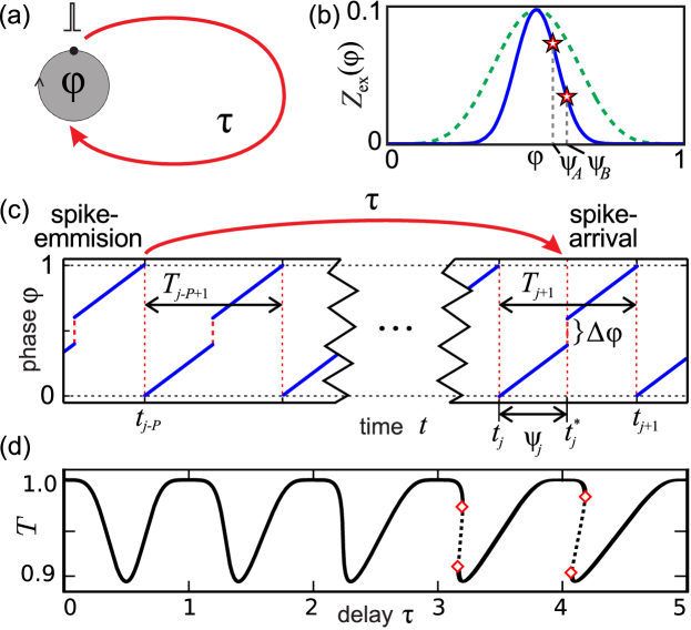
Figure 1: (a) Scheme of the model. (b) Shape of the PRC $Z_{{\rm ex}}(\varphi)$ for $q=5$ (dashed green) and $q=28$ (solid blue). The stars indicate points with slope $-1$. (c) Construction of the map (2): the new ISI $T_{j+1}$ depends on the pulse emitted at $t=t_{j-P}$. (d) Periods $T$ of the RS versus the delay $\tau$ for $q=5$, obtained from Eq. (3). Solid lines indicate stable RS regimes, dashed unstable. Diamonds indicate saddle-node bifurcations.

As a universal and simplest oscillatory spiking model in the absence of the feedback, we consider the phase oscillator $d\varphi/dt=\omega$, where $\varphi\in\mathbb{R}\left(\mod 1\right)$, and $\omega=1$ without loss of generality. When the oscillator reaches $\varphi=1$ at some moment $t$, the phase is reset to zero and the oscillator produces a pulse signal. If this signal is sent into a delayed feedback loop [Fig. 1(a)] the emitted pulses affect the oscillator after a delay $\tau$ at the time instant $t^{*}=t+\tau$. When the pulse is received, the phase of the oscillator undergoes an instantaneous shift by an amount $\Delta\varphi=Z(\varphi(t^{\ast}-0))$, where $Z(\varphi)$ is the phase resetting curve (PRC). Thus, the dynamics of the oscillator can be described by the following equation Canavier2010 ; Goel2002 ; Klinshov2011 ; Lucken2012a ; Luecken2013 :

$$\frac{d\varphi}{dt} = 1+Z(\varphi)\sum\limits_{t_{j}}\delta(t-t_{j}-\tau),$$ (1)

where $t_{j}$ are the instants when the pulses are emitted. Note that we adopt the convention that positive values of the PRC lead to shorter ISIs. For numerical illustrations we use $Z_{{\rm ex}}(\varphi):=0.1\sin^{q}\left(\pi\varphi\right),$ where $q$ controls the steepness of $Z_{{\rm ex}}\left(\varphi\right)$ [see Fig. 1(b)]. However, our analysis is valid for an arbitrary amplitude or shape of the PRC.

In Klinshov2013 it was proven that a system with pulsatile delayed coupling can be reduced to a finite-dimensional map under quite general conditions. To construct the map for system (1) let us calculate the ISI $T_{j+1}:=t_{j+1}-t_{j}$. It is easy to see that $T_{j+1}=1-Z(\psi_{j})$, where $\psi_{j}=\varphi(t_{j}^{\ast}-0)=t_{j}^{*}-t_{j}$ is the phase at the moment of the pulse arrival $t_{j}^{*}=t_{j-P}+\tau$ [Fig. 1(c)]. Here, $P$ is the number of ISIs between the emission time and the arrival time. Substituting $t_{j}=t_{j-P}+T_{j-P+1}+...+T_{j}$, we obtain the ISI map

$$T_{j+1}=1-Z\left(\tau-\sum_{k=j-P+1}^{j}T_{k}\right).$$ (2)

The most basic regime possible in this system is the regular spiking (RS) when the oscillator emits pulses periodically with $T_{j}=T$ for all $j$. Such a regime corresponds to a fixed point of the map (2) and therefore all possible periods $T$ are given as solutions to

$$T=1-Z\left(\tau-PT\right),$$ (3)

where $P=\left[\tau/T\right]$, and hence $\tau-PT=\tau({\rm mod}T)$. Figure 1(d) shows the period $T$ as a function of $\tau$ for $Z_{{\rm ex}}(\varphi)$ and $q=5$.

To analyze the stability of the RS regime, we introduce small perturbations $\delta_{j}$ such that $T_{j}=T+\delta_{j}$, and study whether they are damped or amplified with time. The linearization of (2) in $\delta_{j}$ is straightforward and leads to the characteristic equation

$$\lambda^{P}-\alpha\lambda^{P-1}-\alpha\lambda^{P-2}-...-\alpha\lambda-\alpha = 0,$$ (4)

where $\alpha:=Z^{\prime}(\psi)$ is the slope of the PRC at the phase $\psi=\tau\mod T$ (cf. Canavier2010 ; Foss2000 ).

There are two possibilities for the multipliers $\lambda$ to become critical, i.e. $\left|\lambda\right|=1$. The first scenario takes place at $\alpha=1/P$ when the multiplier $\lambda=1$ appears, which indicates a saddle-node bifurcation [diamonds in Fig. 1(d)]. In general these folds of the RS-branch lead to the appearance of multistability and hysteresis between different RS regimes Foss2000 ; Foss1996 ; Hashemi2012 .

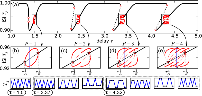
Figure 2: (a) ISIs $T_{j}$ versus the delay $\tau$ for (1) with $Z=Z_{{\rm ex}}$ and $q=28$. Solid lines correspond to stable, dashed and dotted to unstable solutions. Black color indicates RS regimes, red stands for bipartite solutions (with two different ISIs). Diamonds indicate saddle-node bifurcations and stars multi-jitter bifurcations. (b), (c), (d), and (e) are zooms of (a) for $P=1,2,3,4$. The lower panels show examples of stable bipartite solutions, for which the corresponding sequences of ISIs are plotted versus time. Solutions within the same dashed frame coexist at a common value of $\tau$, which is also indicated by a vertical blue line in the corresponding zoom.

The second scenario is much more remarkable and takes place at $\alpha=-1$, where $P$ critical multipliers $\lambda_{k}=e^{i2\pi k/(P+1)},$ $1\leq k\leq P$, appear simultaneously. This feature is quite unusual since in general bifurcations one would not expect more than one real or two complex-conjugate Floquet multipliers become critical at once Kuznetsov1995 . In the following we study this surprising bifurcation in detail and explain why we call it ”multi-jitter”.

In order to observe the multi-jitter bifurcation, the PRC $Z(\varphi)$ must possess points with sufficiently steep negative slope $Z^{\prime}(\varphi)=-1$. For instance, in the case $Z(\varphi)=Z_{{\rm ex}}(\varphi)$, such points exist for $q>q^{*}\approx 27$. For such $q$, two points $\psi_{A},\psi_{B}\in\left(0,1\right)$ exist where $Z_{{\rm ex}}^{\prime}\left(\psi_{A,B}\right)=-1$ [see stars in Fig. 1(b)]. This means that for appropriate values of the delay time $\tau$, such that $\tau\left({\rm mod}T\right)\in\{\psi_{A},\psi_{B}\}$, it holds $\alpha=-1$, and the multi-jitter bifurcation takes place. Using Eq. (3) one may determine the corresponding values of $\tau$ for each possible $P\geq 1$:

$$\tau_{A,B}^{P}=P(1-Z(\psi_{A,B}))+\psi_{A,B}.$$ (5)

Figure 2 shows the numerically obtained bifurcation diagram for $q=28$. All values of its ISIs $T_{j}$ observed after a transient are plotted by solid lines versus the delay $\tau$. Black lines correspond to RS regimes, while irregular regimes with distinct ISIs are indicated in red color. Black dashed lines correspond to unstable RS solutions obtained from Eq. (3). For the intervals $\tau\in(\tau_{A}^{P},\tau_{B}^{P})$, the RS regime destabilizes and several stable irregularly spiking regimes appear.

Let us study in more detail the bifurcation points $\tau=\tau_{A,B}^{P}$ for different values of $P$. For $P=1$, only one multiplier $\lambda=-1$ becomes critical. Note that in this case the map (2) is one-dimensional and the corresponding bifurcation is just a supercritical period doubling giving birth to a stable period-2 solution existing in the interval $\tau\in(\tau_{A}^{1},\tau_{B}^{1})$ [Fig. 2(b)]. For this solution the ISIs $T_{j}$ form a periodic sequence $(\overline{\Theta_{1},\Theta_{2}})$, where the periodicity of the sequence is indicated by an overline. It satisfies

$$\Theta_{2}=1-Z\left(\tau-\Theta_{1}\right)\text{ and }\Theta_{1}=1-Z\left(\tau-\Theta_{2}\right).$$ (6)

For $P\geq 2$, $P$ multipliers become critical simultaneously at $\tau=\tau_{A,B}^{P}$ and the RS solution is unstable for $\tau\in(\tau_{A}^{P},\tau_{B}^{P})$. Numerical study shows that various irregular spiking regimes appear in this interval. We observe solutions, which have ISI sequences of period $P+1$ but exhibit only two different ISIs in varying order [see Fig. 2, bottom]. As a result, each solution corresponds to only two, and not $P+1$, points in Figs. 2(a),(c)–(e). In the following we call such solutions “bipartite”. For larger $P$, a variety of different bipartite solutions with $(P+1)$-periodic ISI sequences can be observed in $\tau\in(\tau_{A}^{P},\tau_{B}^{P})$. The stability regions of these solutions alternate and may overlap leading to multistable regimes [see Appendix, Figs.A.1–A.4].

The bipartite structure of the observed solutions can be explained by their peculiar combinatorial origin. Indeed, all bipartite solutions can be constructed from the period-2 solution$(\overline{\Theta_{1},\Theta_{2}})$ existing for $P=1.$ Consider an arbitrary $(P+1)$-periodic sequence of ISIs $(\overline{T_{1},T_{2},...,T_{P+1}})$, where each $T_{j}$ equals one of the solutions $\Theta_{1,2}$ of (6) for some delay $\tau=\tau_{0}\in\left[\tau_{A}^{1},\tau_{B}^{1}\right]$. Let $n_{1}\geq 1$ and $n_{2}\geq 1$ be the number of ISIs equal to $\Theta_{1}$ and to $\Theta_{2}$ respectively. Then it is readily checked that the constructed sequence is a solution of (2) at the feedback delay time

$$\tau_{n_{1},n_{2}}=\tau_{0}+\left(n_{1}-1\right)\Theta_{1}+\left(n_{2}-1\right)\Theta_{2}.$$ (7)

Red dotted lines in Figs. 2(c), (d), and (e) show the branches of bipartite solutions constructed from (6) with $P=n_{1}+n_{2}-1=2,3,4$. Note that these solutions lie exactly on the numerical branches which validates the above reasoning. However, some parts of the branches are unstable and not observable. Since each bipartite solution corresponds to a pair of points $\left(\tau_{n_{1},n_{2}},T_{1}\right)$ and $\left(\tau_{n_{1},n_{2}},T_{2}\right)$, solutions with identical $n_{1}$ and $n_{2}$ correspond to the same points in the bifurcation diagrams in Fig. 2. For instance, when $P=3$ the branches corresponding to the solutions $(\overline{\Theta_{1},\Theta_{2},\Theta_{1},\Theta_{2}})=(\overline{\Theta_{1},\Theta_{2}})$ and $(\overline{\Theta_{1},\Theta_{1},\Theta_{2},\Theta_{2}})$ lie on top of each other.

Let us estimate the number of different bipartite solutions for a given $P\in\mathbb{N}$. The number of different binary sequences of the length $P+1$ equals $2^{P+1}$. Subtracting the two trivial sequences corresponding to the RS one gets $2^{P+1}-2$. Disregarding the possible duplicates by periodic shifts (maximally $P+1$ per sequence) one obtains an estimate for the total number ${\cal N}_{P}$ of bipartite solutions for a given value of $P$ as

$${\cal N}_{P}\geq\frac{2^{P+1}-2}{(P+1)}.$$ (8)

Notice that all these bipartite solutions exist at the same value of $P$ but for different ranges of the delay $\tau$. Nevertheless, all emerge from the RS solution in the bifurcation points $\tau_{A,B}^{P}$. To see this, let us consider the limit $\tau_{0}\to\tau_{A}^{1}$. In this case the ISIs $\Theta_{1}(\tau_{0})$ and $\Theta_{2}(\tau_{0})$ tend to the same limit $T_{A}=1-Z\left(\psi_{A}\right)$ which is the period of the RS at the bifurcation point. Then, (7) converges to $\tau_{A}^{1}+(n_{1}+n_{2}-2)T_{A}=\tau_{A}^{P}$, while all bipartite solutions converge to the RS with period $T_{A}$.

Thus, all bipartite solutions branch off the RS in the bifurcation points $\tau_{A,B}^{P}$. This finding is clearly recognizable in Figs. 2(c)–(e), where stars indicate the multi-jitter bifurcation points. Numerical simulations show that many of the bipartite solutions stabilize leading to high multistability. In particular, we observe that all bipartite solutions with same values of $n_{1}$ and $n_{2}$ exhibit identical stability. This emergence of numerous irregular spiking, or jittering, regimes motivates the choice of the name “multi-jitter bifurcation”.

High multistability is a well-known property of systems with time delays. A common reason is the so-called reappearance of periodic solutions Yanchuk2009 . This mechanism may cause multistability of coexisting periodic solutions, whose number is linearly proportional to the delay. Due to multi-jitter bifurcation, multistability can develop much faster, since the number of coexisting solutions grows exponentially with the delay [cf. Eq. (8)]. This suggests that the underlying mechanism is quite different.

Irregular spiking regimes similar to the ones described here were reported previously for systems exhibiting a dynamical “memory effect”, where the effect of each incoming pulse lasts for several periods Glass . In system (1), however, the effect of a pulse decays completely within one period. Therefore the origin of jittering must be different. In fact, it relies on another kind of memory, which is provided by the delay line and stores the last $P$ ISIs. This memory preserves fundamental properties of time, which are responsible for the degeneracy of the multi-jitter bifurcation. To explain this let us consider (2) as a $P$-dimensional mapping $\left(T_{j-P+1},...,T_{j}\right)\mapsto\left(T_{j-P+2},...,T_{j+1}\right).$ Disregarding the calculation of the new ISI $T_{j+1}$ as in (2), all the map does is to move the timeframe by shifting all ISIs one place ahead. The rigid nature of time allows no physically meaningful modification of this part of the map which could unfold the degenerate bifurcation. Moreover, the new ISI $T_{j+1}$ depends exclusively on the sum of the previous ISIs which has the effect that all past intervals have an equal influence on the new ISI regardless of their order. As a consequence the combinatorial accumulation of coexisting solutions with differently ordered ISIs is generated.

Besides the delayed feedback, another essential ingredient for the multi-jitter bifurcation is the existence of points where the PRC fulfills $Z^{\prime}(\varphi)<-1$. Since the PRC is a characteristic that can be measured for an arbitrary oscillator Winfree2001 , this condition gives a practical criterion for the occurence of jittering regimes. In this context it is worth noticing that the condition $Z^{\prime}(\varphi)<-1$ is equivalent to the non-monotonicity of the system’s response to an external pulse, i.e. there are such phases $\varphi_{1}<\varphi_{2}$ that a pulse can reverse their order as $\varphi_{1}+Z(\varphi_{1})>\varphi_{2}+Z(\varphi_{2})$. Note that for a smooth one-dimensional system as (1) the reversal of phases is only possible if the feedback takes the form of $\delta$-pulses. With pulses of finite duration two continuous orbits connecting the different phase values before and after the pulse cannot cross each other. This prevents a reversal of phases. However, for oscillators with a phase space of dimension larger than one the phase points $\varphi_{1}$ and $\varphi_{2}$ can exchange their order without necessitating the orbits to intersect.

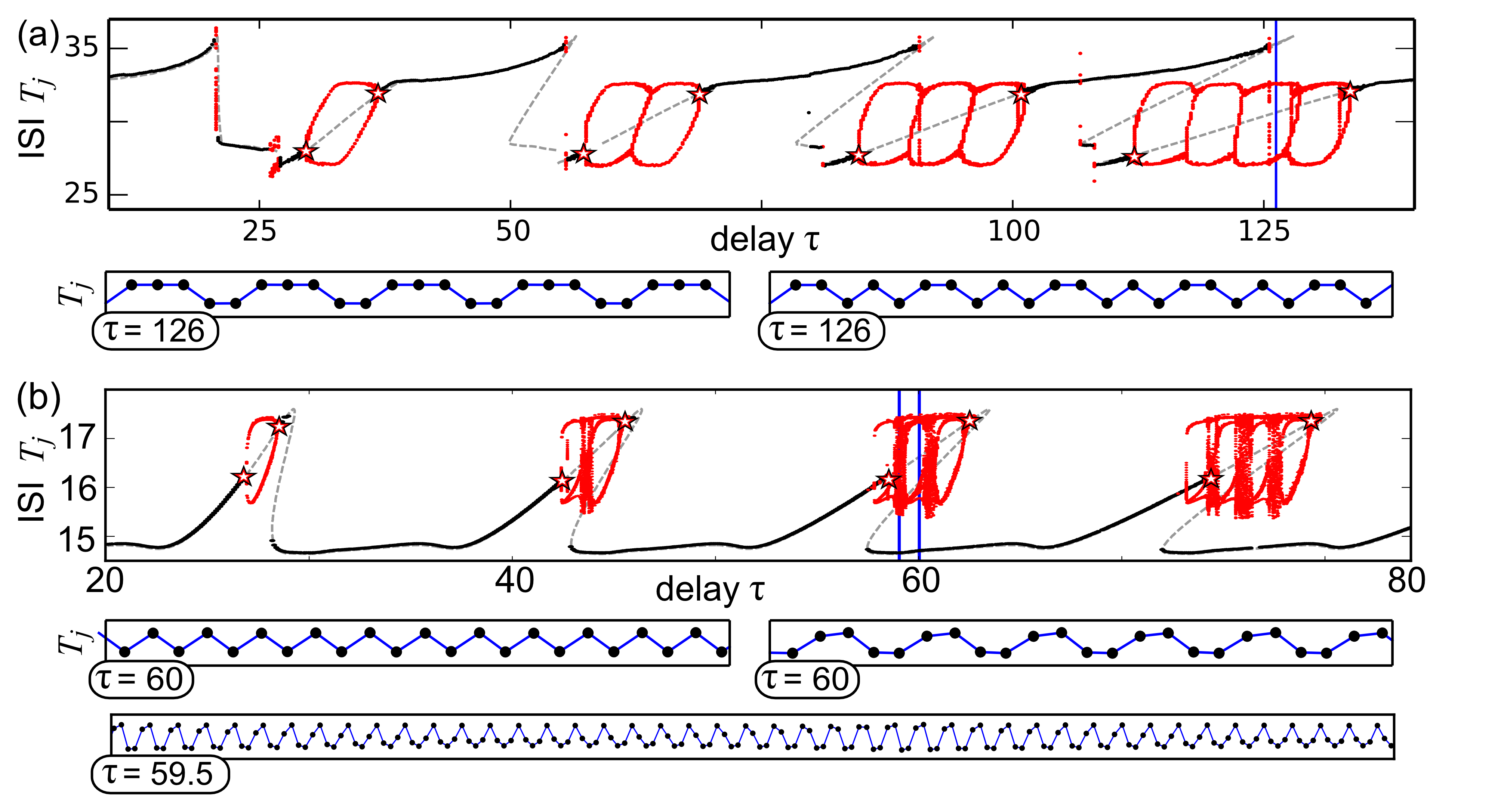
Figure 3: Bifurcation diagrams for (a) an electrically implemented FitzHugh-Nagumo system and (b) a simulated Hodgkin-Huxley neuron model. RS solutions are indicated by black dots, solutions with more than one ISI by red dots. The branches of RS solutions obtained from the measured PRCs and (3) are plotted as dashed grey lines. Multi-jitter bifurcations are indicated by star-shaped markers. The values of the delay $\tau$ are given in ms. The panels below the diagrams show examples of stable bipartite solutions (ISIs versus time). The values of $\tau$ for which the solutions exist are also indicated by vertical blue lines in the corresponding diagrams.

In order to evaluate the practical relevance of the theory described above we consider two realistic systems: (i) an electronic implementation of the FitzHugh-Nagumo oscillator FitzHugh1961 ; Binczak2003 ; shchapin2009dynamics ; Klinshov2014 with time-delayed pulsatile feedback, and (ii) a numerically simulated Hodgkin-Huxley model Hodgkin1952 with a delayed, inhibitory, chemical synapse projecting onto itself Foss2000 ; Hashemi2012 . A detailed description of the systems is given in the Appendix [Secs. B and C]. In both cases the measured PRC exhibits parts with slope less than $-1$ [ see Figs. B.1 and C.1]. Therefore the existence of multi-stable jittering can be conjectured on the basis of our results for system (1). Figure 3 presents experimentally (for the FitzHugh-Nagumo oscillator) and numerically (for the Hodgkin-Huxley model) obtained bifurcation diagrams showing ISIs for varying delays. Both systems clearly show that a stable RS solution destabilizes closely to the multi-jitter bifurcation points. Where the RS regime is unstable, the system switches to irregular spiking, and we mainly observe $(P+1)$-periodic bipartite solutions. The insets in the lower part of Fig. 3(a) show two such period-5 bipartite regimes of the FitzHugh-Nagumo oscillator. Note that both of them coexist at $\tau=126$ ms, which illustrates the multistability of the system. Similarly, two period-4 bipartite regimes coexisting for $\tau=60$ ms for the Hodgkin-Huxley model are shown in 3(b).

Bipartite solutions are a basic form of jittering both in phase-reduced models and realistic systems. However, beyond the multi-jitter bifurcation the bipartite solutions may undergo subsequent bifurcations. In system (1), we observed higher-periodic, quasiperiodic and chaotic regimes for larger steepnesses of the PRC ($q>70$). Similar regimes were also found for the Hodgkin-Huxley model. An example showing aperiodic jittering is shown in Fig.  3(b) for $\tau=59.5$ ms. In the Appendix we show more examples of aperiodic jittering [see Fig. D.1].

To conclude, in a phase oscillator with delayed pulsatile feedback (1) we discovered a surprising bifurcation leading to the emergence of a large number ($\sim\exp\tau$) of jittering solutions. We showed that this multi-jitter bifurcation does not only appear in phase-reduced models, but also in realistic neuron models and even in physically implemented electronic systems. These findings support our theoretical results and provide motivation for a deeper study of the multi-jitter phenomenon.

The possibility of jittering depends on the steepness of the PRC which is an easily measurable quantity for most oscillatory systems Winfree2001 . Thus, our findings provide an easy criterion to check for the existence of jittering in a given system. This may prove useful in a variety of research areas, where pulsatile feedback or interactions of oscillating elements takes place. For instance, this might be one of the mechanisms behind the appearance of irregular spiking in neuronal models with delayed feedback Ma2007 and timing jitter in semiconductor laser systems with delayed feedback Otto2012 . For applications which exploit complex transient behavior such as liquid state machines LSM the high dimension of the unstable manifold at the bifurcation can be interesting. Furthermore, in view of the possibility of a huge number of coexisting attracting orbits beyond the bifurcation the system can serve as a memory device by associating inputs with the attractors to which they make the system converge.

Appendix A Maps and basins for $P=1,2,3,4$

In this section we illustrate the ISI maps for cases $P=1,2,3,4$. In all cases we use $Z_{{\rm ex}}(\varphi):=0.1\sin^{q}\left(\pi\varphi\right)$ with $q=28$.

$\boldsymbol{P=1.}$ In this case the map is one-dimensional:

$$T_{j+1}=1-Z\left(\tau-T_{j}\right).$$ (A.1)

The dynamics of the map can be illustrated on a coweb diagram which is depicted in Fig. A.1 for $\tau=1.5.$ For this value of the delay, the only attractor is a stable period 2 solution [cf. Fig. 2 of the main text].

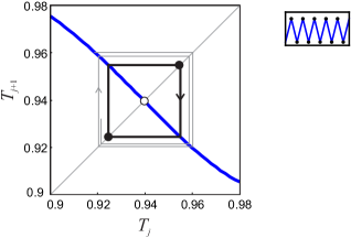
Figure A.1: Cob-web diagram of (A.1) for $\tau=1.5$. The black solid dots correspond to a stable period 2 solution and the white hallow dot corresponds to unstable regular spiking.

$\boldsymbol{P=2.}$ In this case the map is two-dimensional and reads

$$T_{j+1}=1-Z\left(\tau-T_{j}-T_{j-1}\right).$$ (A.2)

This can be equally rewritten in the vector form:

$$\left(\begin{array}[]{c}T_{1}\\ T_{2}\end{array}\right)\mapsto\left(\begin{array}[]{c}T_{2}\\ 1-Z\left(\tau-T_{2}-T_{1}\right)\end{array}\right).$$

Figure A.2 shows attractors and their attraction basins of the map (A.2) for $\tau=2.414$. For this value of the delay we observe a coexistence of a stable regular spiking solution and a stable irregular period-3 solution of the form $(\overline{\Theta_{1},\Theta_{1},\Theta_{2}})$ [cf. Eq. 6 of the main text].

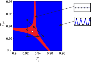
Figure A.2: Phase plane of (A.2) for $\tau=2.414$. The black solid dots correspond to a stable period 3 solution and the white hallow dot corresponds to stable regular spiking. The blue region is the attraction basin of the period-3 solutions, red of regular spiking.

$\boldsymbol{P=3.}$ In this case the map is three-dimensional and reads

$$T_{j+1}=1-Z\left(\tau-T_{j}-T_{j-1}-T_{j-2}\right),$$ (A.3)

or, written in an equivalent vector form

$$\left(\begin{array}[]{c}T_{1}\\ T_{2}\\ T_{3}\end{array}\right)\to\left(\begin{array}[]{c}T_{2}\\ T_{3}\\ 1-Z\left(\tau-T_{3}-T_{2}-T_{1}\right)\end{array}\right).$$

For $\tau=3.37$ three different stable bipartite solutions of this map coexist: $(\overline{\Theta_{1},\Theta_{1},\Theta_{1},\Theta_{2}})$, $(\overline{\Theta_{1},\Theta_{1},\Theta_{2},\Theta_{2}})$, and $(\overline{\Theta_{1},\Theta_{2}})$. Figure A.3 depicts the basins of attractions confined to the two-dimensional plane

$$H=\{(T_{1},T_{2},T_{3})\,|\,\,T_{1},T_{2}\in[0.9,0.98],T_{3}=T_{1}\}$$ (A.4)

of the three-dimensional phase space.

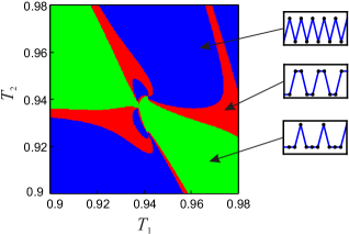
Figure A.3: Planar section of the attractor basins of the map (A.3) by the plane (A.4) for $\tau=3.37$. The corresponding attracting bipartite solutions are depicted in the right part.

$\boldsymbol{P=4.}$ In this case the map is four-dimensional and has the form

$$T_{j+1}=1-Z\left(\tau-T_{j}-T_{j-1}-T_{j-2}-T_{j-3}\right).$$ (A.5)

Here we omit the vector form for brevity. For $\tau=4.32$ four different stable bipartite solutions coexist: $(\overline{\Theta_{1},\Theta_{1},\Theta_{2},\Theta_{2},\Theta_{2}})$, $(\overline{\Theta_{1},\Theta_{2},\Theta_{1},\Theta_{2},\Theta_{2}})$, $(\overline{\Theta_{1},\Theta_{1},\Theta_{1},\Theta_{2},\Theta_{2}})$, and $(\overline{\Theta_{1},\Theta_{1},\Theta_{2},\Theta_{1},\Theta_{2}})$. An intersection of the attractors basins with the 2-dimensional plane

$$H=\{(T_{1},T_{2},T_{3},T_{4})|\,T_{1},T_{2}\in[0.9,0.98],T_{3}=T_{1},T_{4}=T_{2}\}$$ (A.6)

is shown in Fig. A.4.

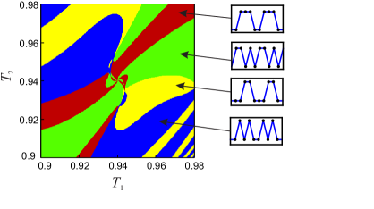
Figure A.4: Planar section of the attractor basins by the plane (A.6) of the map (A.5) for and $\tau=4.32$. The corresponding attracting bipartite solutions are depicted in the right part.

Appendix B Electronic FitzHugh-Nagumo oscillator

The circuitry of the electronic FitzHugh-Nagumo oscillator as used in the experiment [cf. Fig. 3(a) of the main text] is depicted in Fig. B.1(a), see Refs. shchapin2009dynamics ; Klinshov2014 for details. Here, $R=1$k$\Omega$, $C=47$nF, $L=103.4$H, $P_{in}$ is an input from the delay line, and $F(u)=\alpha u(u-u_{0})(u+u_{0})$ is the current-voltage characteristic of the nonlinear resistor with $\alpha=2.02\times 10^{-4}\Omega^{-1}\mbox{V}^{-1}$ and $u_{0}=0.82$V. The autonomous oscillations have period $T\approx 30$ms. The delay line is realized as a chain of monostable multivibrators. A pulse of the amplitude $A=5$V and duration $\theta=0.42$ms is delivered with a delay $\tau$ each time the voltage $u$ reaches the threshold $u_{th}=-0.7$V.

The noise level in the circuit was $\approx-40$dB (this means fluctuations of $\approx 20$mV for a signal amplitude of $\approx 2$V).

The measured phase resetting curve for the given parameters is depicted in Fig. B.1(b). The interval where the PRC slope is less than minus one is highlighted in red.

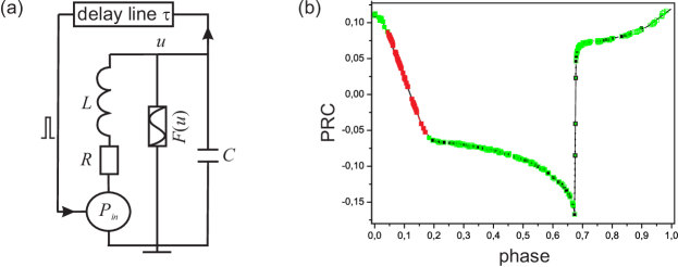
Figure B.1: (a) Circuitry of the Fitzhugh-Nagumo oscillator. (b) The measured PRC of the FitzHugh-Nagumo oscillator. The interval with the slope less than minus one is highlighted in red.

Appendix C Hodgkin-Huxley model

The periodically spiking Hodgkin-Huxley neuron model, which was used for the numericalresults in Fig. 3(b) of the main text, is given by the following set of equations Foss2000 ; Hashemi2012 ; Hodgkin1952

$$C\dot{V}(t) =I-g_{Na}m^{3}h(V(t)-V_{Na})-g_{K}n(V(t)-V_{K})$$

$$-g_{l}(V(t)-V_{l})-\kappa(V(t)-V_{r})s(t-\tau),$$ (C.1)

$$\dot{m}(t) =\alpha_{m}(V(t))(1-m(t))-\beta_{m}(V(t))m(t),$$

$$\dot{h}(t) =\alpha_{h}(V(t))(1-h(t))-\beta_{h}(V(t))h(t),$$

$$\dot{n}(t) =\alpha_{n}(V(t))(1-n(t))-\beta_{n}(V(t))n(t),$$

$$\dot{s}(t) =5(1-s(t))/(1+\exp(-V(t)))-s(t),$$

where $V(t)$ models the membrane potential, $\alpha_{m}(V)=(0.1V+4)/(1-\exp(-0.1V-4))$, $\beta_{m}(V)=4\exp((-V-65)/18)$, $\alpha_{h}=0.07\exp((-V-65)/20)$, $\beta_{h}(V)=1/(1+\exp(-0.1V-3.5))$, $\alpha_{n}(V)=(0.01V+0.55)/(1-\exp(-0.1V-5.5))$, $\beta_{n}(V)=0.125\exp((-V-65)/80)$, $C=1\mu\text{F}/\text{cm}^{2}$, $I=10\mu\text{A}/\text{cm}^{2}$, $g_{Na}=120\text{mS}/\text{cm}^{2}$, $V_{Na}=50\text{mV}$, $g_{K}=36\text{mS}/\text{cm}^{2}$, $V_{K}=-77\text{mV}$, $g_{l}=0.3\text{mS}/\text{cm}^{2}$, $V_{l}=-54.5\text{mV}$, $V_{r}=-65\text{mV}$, and $\kappa=0.38\text{mS}/\text{cm}^{2}$.

Figure C.1 shows the PRC of (C.1), which was measured by replacing the delayed feedback by an external stimulation line through which singular synaptic pulses sampled from the same system were applied at different phases.

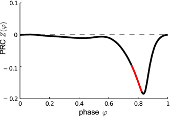
Figure C.1: PRC of the Hodgkin-Huxley model (C.1). The region, where $Z^{\prime}\left(\varphi\right)<-1$ is indicated by red.

Appendix D Emergence of chaotic jittering in the Hodgkin-Huxley model

Figure D.1 illustrates the emergence of chaotic jittering states for increasing feedback strength $\kappa$. It shows three different trajectories for $\tau=59.3$ and $\kappa=0.38,\,0.4,\,0.41$. In plot (a), the ISIs of a quasiperiodic solution are shown for $c=0.38$. A black dot is placed at $(t_{j},T_{j})$, where $t_{j}$ is the moment when the $j$-th ISI ends and $T_{j}$ is its duration. Subsequent dots are joined by a blue line. The sequence is contained in a torus in the phase-space, whose projection to the $(T_{j},T_{j+1})$-plane is shown in plot (b). For each $T_{j}$ from the sequence of approximately thousand observed ISIs, a blue dot was placed at the coordinates $(T_{j},T_{j+1})$. Plots (c) and (d) depict a solution close to the onset of chaotic jittering for $c=0.4$. The corresponding Lyapunov exponent is positive but small [see Fig. D.2(b)]. A more pronounced chaos is exhibited by the solution existing at $c=0.41$, which is shown in plots (e) and (f). Note that the emergence of chaos is accompanied by a loss of smoothness of the torus consisting of the quasiperiodic trajectories Afra2003 .

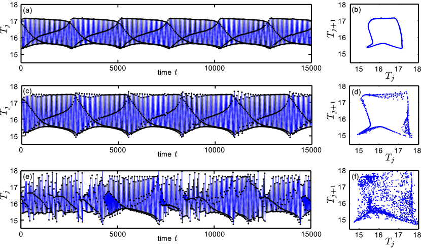
Figure D.1: Emergence of chaotic jittering in (C.1). The plots (a), (c), and (e) show ISI sequences of trajectories observed at the indicated feedback strengths $\kappa=0.38,\,0.4,\,0.41$. (a),(b): Quasiperiodic jittering for $c=0.38$; (c),(d): weakly chaotic jittering for $c=0.4$; (e),(f): clearly recognizable chaotic jittering for $c=0.41$.

Figure D.2 shows the numerically calculated Lyapunov exponents (LE) for different values of the feedback strength $\kappa$. For each value of $\kappa$ the four largest exponents are shown. Starting from $\tau=58$ on the RS solution with maximal period [cf. Fig. 3(b) for $\kappa=0.38$] each computation for $\tau\in[58,60.5]$ was initialized with a solution on the previous attractor as initial data. Note that there exists always one LE which has real part zero, since the corresponding attractors are not steady states. For each value of $\tau$, the point where the multi-jitter bifurcation occurs can clearly be recognized as all four depicted LE approach zero nearly at the same value of $\tau=\tau_{A}$ ($\tau_{A}\approx 58.75$ for $\kappa=0.38$, $\tau_{A}\approx 58.4$ for $\kappa=0.4$, and $\tau_{A}\approx 58.3$ for $\kappa=0.41$). Dynamics found in the depicted range beyond these points, i.e. for $\tau_{A}<\tau<60.5$, are irregularly spiking regimes. For $\kappa=0.38$, two LE are zero in the interval $\tau\in[59.25,59.8]$, which indicates a torus, i.e. quasiperiodic behavior as illustrated in Fig. D.1(a). For all other values of $\tau$ in the depicted range, we observe periodic solutions which exhibit ISI sequences of period 4 [see Fig.3(b) of the main text]. When the feedback strength is increased to $\kappa=0.4$ the dynamics in the corresponding interval $\tau\in[59.2,59.5]$ become weakly chaotic. For $\kappa=0.41$ the LE become larger in the interval $\tau\in[58.75,59.2]$ which indicates a more pronounced chaos. Note that even for feedback strengths where chaotic jittering is observed, periodic solutions still exist at other values of $\tau$.

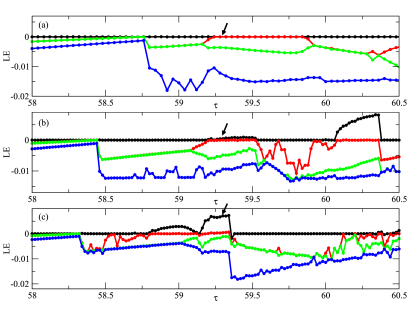
Figure D.2: Four largest Lyapunov exponents of (C.1) with $\tau\in[58,60.5]$ and feedback strengths (a) $\kappa=0.38$; (b) $\kappa=0.4$; (c) $\kappa=0.41$. Arrows indicate the delays, for which the trajectories in Fig. D.1 are shown.