Universal formula for the flavor non-singlet axial-vector current from the gradient flow

Abstract

By employing the gradient/Wilson flow, we derive a universal formula that expresses a correctly normalized flavor non-singlet axial-vector current of quarks. The formula is universal in the sense that it holds independently of regularization and especially holds with lattice regularization. It is also confirmed that, in the lowest non-trivial order of perturbation theory, the triangle diagram containing the formula and two flavor non-singlet vector currents possesses non-local structure that is compatible with the triangle anomaly.

B01, B31, B32, B38

1 Introduction

In this paper, we consider a well-studied problem, how to construct a correctly (or canonically) normalized flavor non-singlet axial-vector current of quarks, in a new light using the gradient/Wilson flow Luscher:2010iy ; Luscher:2011bx ; Luscher:2013cpa . An axial-vector current $j_{5\mu}^{A}(x)$ is said to be correctly normalized, if it fulfills the Ward–Takahashi relation associated with the flavor chiral symmetry. That partially conserved axial current (PCAC) relation is

$$\left\langle\partial_{\mu}j_{5\mu}^{A}(x)\psi(y)\bar{\psi}(z)\right\rangle-\left\langle\bar{\psi}(x)\gamma_{5}\{t^{A},M_{0}\}\psi(x)\psi(y)\bar{\psi}(z)\right\rangle$$

$$=-\delta^{4}(y-x)\gamma_{5}t^{A}\left\langle\psi(y)\bar{\psi}(z)\right\rangle-\delta^{4}(z-x)\left\langle\psi(y)\bar{\psi}(z)\right\rangle\gamma_{5}t^{A},$$ (1.1)

where $\psi$ and $\bar{\psi}$ are quark and anti-quark fields and $t^{A}$ ($A=1$, …, $N_{f}^{2}-1$) denotes the generator of the flavor $SU(N_{f})$ group. $M_{0}$ is the (flavor-diagonal) bare quark mass matrix. This relation says that the axial-vector current $j_{5\mu}^{A}(x)$ generates the axial part of the flavor symmetry $SU(N_{f})_{L}\times SU(N_{f})_{R}$ in the correct magnitude. The construction of such a composite operator is, however, not straightforward because a regulator that manifestly preserves the chiral symmetry does not easily come to hand. The only known explicit examples of such chiral-symmetry-preserving regularization are the domain-wall lattice fermion Kaplan:1992bt ; Shamir:1993zy ; Furman:1994ky and the overlap lattice fermion Neuberger:1997fp ; Neuberger:1998wv , both satisfy the Ginsparg–Wilson relation Ginsparg:1981bj ; Hasenfratz:1998jp ; Hasenfratz:1998ri ; Luscher:1998pqa .

For example, if one uses dimensional regularization with complex dimension $D=4-2\epsilon$ and

$$\gamma_{5}=\gamma_{0}\gamma_{1}\gamma_{2}\gamma_{3},$$ (1.2)

a simple expression for the axial-vector current

$$\bar{\psi}(x)\gamma_{\mu}\gamma_{5}t^{A}\psi(x)$$ (1.3)

does not fulfill Eq. (1.1). Instead one finds (see Ref. Collins:1984xc , for example)

$$\left\langle\partial_{\mu}\left[\bar{\psi}(x)\gamma_{\mu}\gamma_{5}t^{A}\psi(x)\right]\psi(y)\bar{\psi}(z)\right\rangle-\left\langle\bar{\psi}(x)\gamma_{5}\{t^{A},M_{0}\}\psi(x)\psi(y)\bar{\psi}(z)\right\rangle$$

$$=-\delta^{4}(y-x)\gamma_{5}t^{A}\left\langle\psi(y)\bar{\psi}(z)\right\rangle-\delta^{4}(z-x)\left\langle\psi(y)\bar{\psi}(z)\right\rangle\gamma_{5}t^{A}$$

$$\qquad{}+\frac{g_{0}^{2}}{(4\pi)^{2}}C_{2}(R)4\left\langle\partial_{\mu}\left[\bar{\psi}(x)\gamma_{\mu}\gamma_{5}t^{A}\psi(x)\right]\psi(y)\bar{\psi}(z)\right\rangle$$

$$\qquad\qquad{}-\frac{g_{0}^{2}}{(4\pi)^{2}}C_{2}(R)8\left\langle\bar{\psi}(x)\gamma_{5}\{t^{A},M_{0}\}\psi(x)\psi(y)\bar{\psi}(z)\right\rangle+O(g_{0}^{4})$$ (1.4)

for $\epsilon\to 0$. This relation shows that under dimensional regularization, the correctly normalized axial-vector current is not Eq. (1.3) but

$$j_{5\mu}^{A}(x)=\left[1-\frac{g_{0}^{2}}{(4\pi)^{2}}C_{2}(R)4+O(g_{0}^{4})\right]\bar{\psi}(x)\gamma_{\mu}\gamma_{5}t^{A}\psi(x)$$ (1.5)

in conjunction with a redefinition of the pseudo-scalar density,

$$\left[1-\frac{g_{0}^{2}}{(4\pi)^{2}}C_{2}(R)8+O(g_{0}^{4})\right]\bar{\psi}(x)\gamma_{5}\{t^{A},M_{0}\}\psi(x).$$ (1.6)

The relation between the correctly normalized axial-vector current and a bare axial-vector current is regularization-dependent and generally receives radiative corrections in all orders of perturbation theory. If one changes regularization (to lattice regularization with a particular discretization of the Dirac operator, for example), one has to compute the corresponding relation anew.

In the present paper, instead, we derive a single “universal formula” that is supposed to hold for any regularization. Our result is

$$j_{5\mu}^{A}(x)=\lim_{t\to 0}\left\{1+\frac{\bar{g}(1/\sqrt{8t})^{2}}{(4\pi)^{2}}C_{2}(R)\left[-\frac{1}{2}+\ln(432)\right]\right\}\mathring{\bar{\chi}}(t,x)\gamma_{\mu}\gamma_{5}t^{A}\mathring{\chi}(t,x).$$ (1.7)

Here, $\bar{g}(q)$ is the running gauge coupling in the minimal subtraction (MS) scheme at the renormalization scale $q$; $\mathring{\chi}(t,x)$ and $\mathring{\bar{\chi}}(t,x)$ are quark and anti-quark fields evolved by flow equations which will be elucidated below. Because of theorems proven in Refs. Luscher:2011bx ; Luscher:2013cpa , the composite operator in the right-hand side of Eq. (1.7) is a renormalized quantity although it is constructed from bare quark fields in a well-defined manner. As far as one carries out the parameter renormalization properly, such a renormalized quantity must be independent of the chosen regularization. In this sense, the formula is “universal.” The formula is also usable with lattice regularization and could be applied for the computation of, say, the pion decay constant.

Since $\bar{g}(1/\sqrt{8t})\to 0$ for $t\to 0$ because of the asymptotic freedom, the formula (1.7) can further be simplified to $j_{5\mu}^{A}(x)=\lim_{t\to 0}\mathring{\bar{\chi}}(t,x)\gamma_{\mu}\gamma_{5}t^{A}\mathring{\chi}(t,x)$. Although this is mathematically correct, practically one cannot simply take the $t\to 0$ limit in lattice Monte Carlo simulations for example. In Eq. (1.7), it is supposed that the regulator is removed (after making the parameter renormalization) and the lower end of the physical flow time $t$ is limited by the lattice spacing as $a\ll\sqrt{8t}$. Thus the asymptotic $t\to 0$ behavior in Eq. (1.7) will be useful to find the extrapolation for $t\to 0$.

The above universal formula for the axial-vector current is quite analogous to universal formulas for the energy–momentum tensor—the Noether current associated with the translational invariance—on the basis of the gradient/Wilson flow Suzuki:2013gza ; Makino:2014taa ; Makino:2014sta ; Suzuki:2015fka ; see also Ref. DelDebbio:2013zaa . The motivation is also similar: Since lattice regularization breaks the translational invariance, the construction of the energy–momentum tensor with lattice regularization is not straightforward Caracciolo:1988hc ; Caracciolo:1989pt . The universal formulas in Refs. Suzuki:2013gza ; Makino:2014taa ; Makino:2014sta ; Suzuki:2015fka , because they are thought to be regularization independent, may be used with lattice regularization. The validity of the formulas has been tested by employing Monte Carlo simulations Asakawa:2013laa ; Kitazawa:2014uxa and the $1/N$ expansion Makino:2014cxa (see also, Ref. Aoki:2014dxa for the $1/N$ expansion of the gradient flow).

A main technical difference in the derivation of Eq. (1.7) from the derivation of the universal formulas for the energy–momentum tensor in Refs. Suzuki:2013gza ; Makino:2014taa ; Makino:2014sta ; Suzuki:2015fka is that only the knowledge of the one-loop expression in dimensional regularization (1.5) will be used in what follows. On the other hand, in Refs. Suzuki:2013gza ; Makino:2014taa ; Makino:2014sta ; Suzuki:2015fka , full-order perturbative expressions of the correctly normalized energy–momentum tensor (which is readily obtained by dimensional regularization) were used. Although it must be possible to arrive at Eq. (1.7) starting from an “ideal” axial-vector current obtained from the chiral-symmetry-preserving lattice fermions by the Noether method, a much simpler one-loop expression such as Eq. (1.5) is sufficient. This point, we think is technically very interesting.

2 Gradient/Wilson flow

The gradient/Wilson flow Luscher:2010iy ; Luscher:2011bx ; Luscher:2013cpa is an evolution of field configurations according to flow equations with a fictitious time $t$. For the gauge field $A_{\mu}(x)$, the flow is defined by Luscher:2010iy ; Luscher:2011bx

$$\partial_{t}B_{\mu}(t,x)=D_{\nu}G_{\nu\mu}(t,x)+\alpha_{0}D_{\mu}\partial_{\nu}B_{\nu}(t,x),\qquad B_{\mu}(t=0,x)=A_{\mu}(x),$$ (2.1)

where $G_{\mu\nu}(t,x)$ is the field strength of the flowed gauge field $B_{\mu}(t,x)$,

$$G_{\mu\nu}(t,x)=\partial_{\mu}B_{\nu}(t,x)-\partial_{\nu}B_{\mu}(t,x)+[B_{\mu}(t,x),B_{\nu}(t,x)],$$ (2.2)

and the covariant derivative on the gauge field is

$$D_{\mu}=\partial_{\mu}+[B_{\mu},\cdot].$$ (2.3)

The second term in the right-hand side of Eq. (2.1) is a “gauge-fixing term” that is introduced to provide the Gaussian damping factor (see below) to the gauge mode. Although it breaks the gauge covariance, it can be shown that any gauge-invariant quantity is independent of the “gauge parameter” $\alpha_{0}$ Luscher:2010iy .

For the quark fields, $\psi(x)$ and $\bar{\psi}(x)$, the flow is defined by Luscher:2013cpa

$$\partial_{t}\chi(t,x)=\left[\varDelta-\alpha_{0}\partial_{\mu}B_{\mu}(t,x)\right]\chi(t,x),\qquad\chi(t=0,x)=\psi(x),$$ (2.4)

$$\partial_{t}\bar{\chi}(t,x)=\bar{\chi}(t,x)\left[\overleftarrow{\varDelta}+\alpha_{0}\partial_{\mu}B_{\mu}(t,x)\right],\qquad\bar{\chi}(t=0,x)=\bar{\psi}(x),$$ (2.5)

where covariant derivatives for the flowed quark field, $\chi(t,x)$ and $\bar{\chi}(t,x)$, are

$$\varDelta=D_{\mu}D_{\mu},\qquad D_{\mu}=\partial_{\mu}+B_{\mu},$$ (2.6)

$$\overleftarrow{\varDelta}=\overleftarrow{D}_{\mu}\overleftarrow{D}_{\mu},\qquad\overleftarrow{D}_{\mu}=\overleftarrow{\partial}_{\mu}-B_{\mu}.$$ (2.7)

For the implementation of these flow equations in lattice gauge theory, see Refs. Luscher:2010iy ; Luscher:2013cpa .

The initial values in above flow equations, $A_{\mu}(x)$, $\psi(x)$, and $\bar{\psi}(x)$, are quantum fields being subject to the functional integral. One can develop Luscher:2010iy ; Luscher:2011bx ; Luscher:2013cpa perturbation theory for quantum correlation functions of the flowed fields, $B_{\mu}(t,x)$, $\chi(t,x)$, and $\bar{\chi}(t,x)$. For example, the tree-level propagator of the flowed gauge field (in the “Feynman gauge” in which $\lambda_{0}=\alpha_{0}=1$, where $\lambda_{0}$ is the conventional gauge-fixing parameter) is

$$\left\langle B_{\mu}^{a}(t,x)B_{\nu}^{b}(s,y)\right\rangle=g_{0}^{2}\delta^{ab}\delta_{\mu\nu}\int_{p}\mathrm{e}^{ip(x-y)}\frac{\mathrm{e}^{-(t+s)p^{2}}}{p^{2}}.$$ (2.9)

Similarly, the tree-level quark propagator is

$$\left\langle\chi(t,x)\bar{\chi}(s,y)\right\rangle=\int_{p}\mathrm{e}^{ip(x-y)}\frac{\mathrm{e}^{-(t+s)p^{2}}}{i{\ooalign{\hfil/\hfil\crcr$p$}}+M_{0}}.$$ (2.10)

The details of the perturbation theory (the flow Feynman rule) are summarized in Ref. Makino:2014taa .

A remarkable feature of the gradient/Wilson flow is its ultraviolet (UV) finiteness Luscher:2011bx ; Luscher:2013cpa . Correlation functions of the flowed gauge field become UV finite without the wave function renormalization (if one makes the parameter renormalization). This finiteness persists even for local products, i.e., composite operators. The flowed quark field, on the other hand requires the wave function renormalization. However, once the elementary flowed quark field is multiplicatively renormalized, any composite operator of it becomes UV finite. Thus, if one introduces the combinations Makino:2014taa

$$\mathring{\chi}(t,x) =\sqrt{\frac{-2\dim(R)N_{f}}{(4\pi)^{2}t^{2}\left\langle\bar{\chi}(t,x)\overleftrightarrow{{\ooalign{\hfil/\hfil\crcr$D$}}}\chi(t,x)\right\rangle}}\,\chi(t,x),$$ (2.13)

$$\mathring{\bar{\chi}}(t,x) =\sqrt{\frac{-2\dim(R)N_{f}}{(4\pi)^{2}t^{2}\left\langle\bar{\chi}(t,x)\overleftrightarrow{{\ooalign{\hfil/\hfil\crcr$D$}}}\chi(t,x)\right\rangle}}\,\bar{\chi}(t,x),$$ (2.16)

where

$$\overleftrightarrow{D}_{\mu}\equiv D_{\mu}-\overleftarrow{D}_{\mu},$$ (2.17)

then wave function renormalization factors are canceled out in $\mathring{\chi}(t,x)$ and $\mathring{\bar{\chi}}(t,x)$ and any local product of them becomes a UV-finite renormalized operator. Thus, if one can express a composite operator in terms of local products of flowed fields, $B_{\mu}(t,x)$, $\mathring{\chi}(t,x)$, and $\mathring{\bar{\chi}}(t,x)$, then the expression provides a universal formula for the composite operator. What we shall do is to apply this idea to the composite operator in Eq. (1.5). An explicit method to rewrite a composite operator in terms of local products of the flowed fields is given by the short flow-time expansion Luscher:2011bx that is the subject of the next section.

3 Small flow-time expansion

We take a would-be axial-vector current composed of the flowed quark field

$$\bar{\chi}(t,x)\gamma_{\mu}\gamma_{5}t^{A}\chi(t,x),$$ (3.1)

and consider its $t\to 0$ limit. As discussed in Ref. Luscher:2011bx , a local product of flowed fields in the $t\to 0$ limit can be expressed by an asymptotic series of local composite operators of fields at zero flow time with increasing mass dimensions. In the present case, because of symmetry, we have

$$\bar{\chi}(t,x)\gamma_{\mu}\gamma_{5}t^{A}\chi(t,x)=c(t)\bar{\psi}(x)\gamma_{\mu}\gamma_{5}t^{A}\psi(x)+O(t)$$ (3.2)

for $t\to 0$.

The expansion can be worked out in perturbation theory; the coefficient $c(t)$ can be found by computing the correlation function

$$\left\langle\bar{\chi}(t,x)\gamma_{\mu}\gamma_{5}t^{A}\chi(t,x)\psi(y)\bar{\psi}(z)\right\rangle$$ (3.3)

and comparing its $t\to 0$ behavior with

$$\left\langle\bar{\psi}(x)\gamma_{\mu}\gamma_{5}t^{A}\psi(x)\psi(y)\bar{\psi}(z)\right\rangle.$$ (3.4)

To one-loop order, there are seven 1PI “flow Feynman diagrams” which contribute to Eq. (3.3); they are depicted in Figs 1–7 according to the convention in Ref. Makino:2014taa .

Figure 1: Diagram a

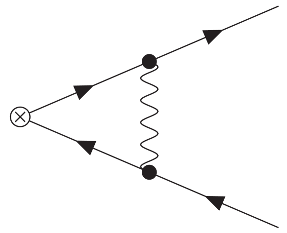
Figure 2: Diagram d

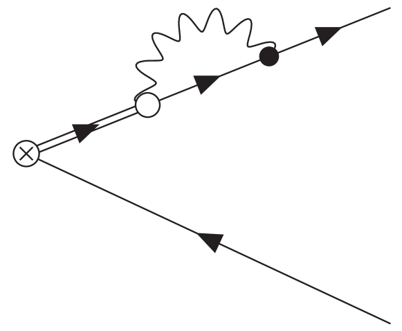
Figure 3: Diagram f

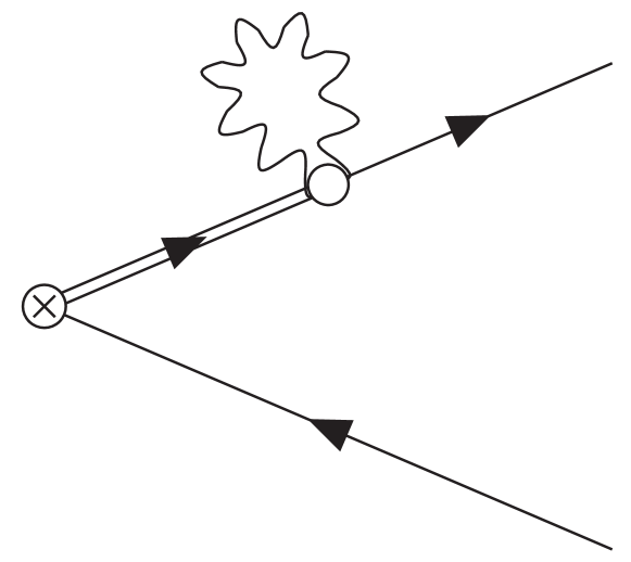
Figure 4: Diagram g

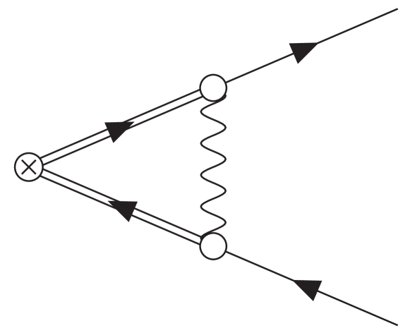
Figure 5: Diagram b

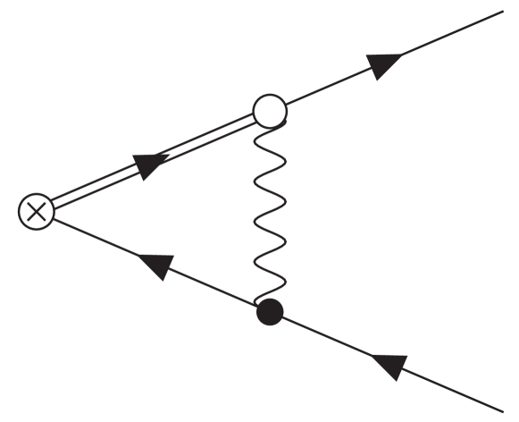
Figure 6: Diagram c

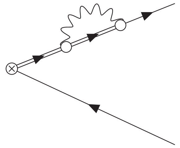
Figure 7: Diagram e

Among these diagrams, diagrams b, c, and e in Figs. 7–7 are irrelevant for the coefficient $c(t)$ in Eq. (3.2) because they are proportional to the momentum of the external quark line. Then, writing Eq. (3.3) as

$$\int\frac{\mathrm{d}^{D}p}{(2\pi)^{D}}\int\frac{\mathrm{d}^{D}q}{(2\pi)^{D}}\,\mathrm{e}^{ip(y-x)}\mathrm{e}^{iq(x-z)}\frac{1}{i{\ooalign{\hfil/\hfil\crcr$p$}}+M_{0}}\mathcal{M}_{5\mu}^{A}(p,q;t)\frac{1}{i{\ooalign{\hfil/\hfil\crcr$q$}}+M_{0}},$$ (3.5)

the contribution of diagram a is $\mathcal{M}_{5\mu}^{A}(0,0;t)=\gamma_{\mu}\gamma_{5}t^{A}$. For one-loop diagrams, we work with dimensional regularization [with the prescription (1.2)]. The contribution of each diagram to $\mathcal{M}_{5\mu}^{A}(0,0;t)$ is tabulated in Table 1.

Table 1: Contribution of each diagram to $\mathcal{M}_{5\mu}^{A}(0,0;t)$ in Eq. (3.5) in units of $\frac{g_{0}^{2}}{(4\pi)^{2}}C_{2}(R)\gamma_{\mu}\gamma_{5}t^{A}$.

d	$(-1)\left[\dfrac{1}{\epsilon}+\ln(8\pi t)+\dfrac{7}{2}\right]$
f	$2\left[\dfrac{1}{\epsilon}+\ln(8\pi t)+1\right]$
g	$(-4)\left[\dfrac{1}{\epsilon}+\ln(8\pi t)+\dfrac{1}{2}\right]$

Combining all the contributions, we have

$$\mathcal{M}_{5\mu}^{A}(0,0;t)=\left\{1+\frac{g_{0}^{2}}{(4\pi)^{2}}C_{2}(R)(-3)\left[\frac{1}{\epsilon}+\ln(8\pi t)+\frac{7}{6}\right]\right\}\gamma_{\mu}\gamma_{5}t^{A}.$$ (3.6)

Invoking a facile method explaining in Ref. Makino:2014taaa , this implies the small flow-time expansion is given by

$$\bar{\chi}(t,x)\gamma_{\mu}\gamma_{5}t^{A}\chi(t,x)$$

$$=\left\{1+\frac{g_{0}^{2}}{(4\pi)^{2}}C_{2}(R)(-3)\left[\frac{1}{\epsilon}+\ln(8\pi t)+\frac{7}{6}\right]\right\}\bar{\psi}(x)\gamma_{\mu}\gamma_{5}t^{A}\psi(x)+O(t).$$ (3.7)

Next we express this in terms of the “ringed” fields in Eqs. (2.13) and (2.16). Using the result of Ref. Makino:2014taa that

$$\frac{-2\dim(R)N_{\mathrm{f}}}{(4\pi)^{2}t^{2}\left\langle\bar{\chi}(t,x)\overleftrightarrow{{\ooalign{\hfil/\hfil\crcr$D$}}}\chi(t,x)\right\rangle}=Z(\epsilon)\left\{1+\frac{g^{2}}{(4\pi)^{2}}C_{2}(R)\left[3\frac{1}{\epsilon}-\varPhi(t)\right]+O(g^{4})+O(t)\right\},$$ (3.8)

where

$$Z(\epsilon)\equiv\frac{1}{(8\pi t)^{\epsilon}},\qquad\varPhi(t)\equiv-3\ln(8\pi\mu^{2}t)+\ln(432),$$ (3.9)

we have for $\epsilon\to 0$,

$$\mathring{\bar{\chi}}(t,x)\gamma_{\mu}\gamma_{5}t^{A}\mathring{\chi}(t,x)$$

$$=\left\{1+\frac{g^{2}}{(4\pi)^{2}}C_{2}(R)\left[-\frac{7}{2}-\ln(432)\right]+O(g^{4})\right\}\bar{\psi}(x)\gamma_{\mu}\gamma_{5}t^{A}\psi(x)+O(t),$$ (3.10)

where we have set $g_{0}^{2}=\mu^{2\epsilon}g^{2}$.

Inverting this relation for $t\to 0$ and plugging it into Eq. (1.6), we have

$$j_{5\mu}^{A}(x)=\left\{1+\frac{g^{2}}{(4\pi)^{2}}C_{2}(R)\left[-\frac{1}{2}+\ln(432)\right]+O(g^{4})\right\}\mathring{\bar{\chi}}(t,x)\gamma_{\mu}\gamma_{5}t^{A}\mathring{\chi}(t,x)+O(t).$$ (3.11)

As the Ward–Takahashi relation (1.1) shows, $j_{5\mu}^{A}(x)$ in the left-hand side of this relation must be UV finite. The right-hand side of this relation is certainly UV finite, as all $1/\epsilon$ singularities are cancelled out.

Finally, we invoke a renormalization group argument. By applying the operation

$$\left(\mu\frac{\partial}{\partial\mu}\right)_{0}$$ (3.12)

to the both sides of Eq. (1.1), where the subscript $0$ implies the bare quantities are kept fixed, we have $(\mu\partial/\partial\mu)_{0}j_{5\nu}^{A}(x)=0$. We also have $(\mu\partial/\partial\mu)_{0}\mathring{\bar{\chi}}(t,x)\gamma_{\mu}\gamma_{5}t^{A}\mathring{\chi}(t,x)=0$, because the flowed quark fields are certain (although very complicated) combinations of bare fields. Therefore, the quantity in the curly brackets in Eq. (3.10) is independent of the renormalization scale $\mu$. This implies that if one uses the running gauge coupling $\bar{g}(q)$ in place of $g$, the expression is independent of the scale $q$. Thus, we set $q=1/\sqrt{8t}$ as a particular choice. Since $\bar{g}(1/\sqrt{8t})\to 0$ for $t\to 0$, the perturbative computation is justified in the $t\to 0$ limit which also eliminates the $O(t)$ term in Eq. (3.11). In this way, we arrive at the universal formula (1.7).

An argument similar to the above may be repeated for the flavor non-singlet pseudo-scalar density that fulfills the PCAC relation,

$$\left\langle\partial_{\mu}j_{5\mu}^{A}(x)\psi(y)\bar{\psi}(z)\right\rangle-\left\langle\left\{\bar{\psi}\gamma_{5}\{t^{A},M\}\psi\right\}_{R}(x)\psi(y)\bar{\psi}(z)\right\rangle$$

$$=-\delta^{4}(y-x)\gamma_{5}t^{A}\left\langle\psi(y)\bar{\psi}(z)\right\rangle-\delta^{4}(z-x)\left\langle\psi(y)\bar{\psi}(z)\right\rangle\gamma_{5}t^{A}.$$ (3.13)

Omitting all details of the calculation, the final result is given by

$$\left\{\bar{\psi}\gamma_{5}\{t^{A},M\}\psi\right\}_{R}(x)$$

$$=\lim_{t\to 0}\left\{1+\frac{\bar{g}(1/\sqrt{8t})^{2}}{(4\pi)^{2}}C_{2}(R)\left[3\ln\pi+2+\ln(432)\right]\right\}\mathring{\bar{\chi}}(t,x)\gamma_{5}\{t^{A},\bar{M}(1/\sqrt{8t})\}\mathring{\chi}(t,x).$$ (3.14)

In these expressions, the MS or $\overline{\text{MS}}$ scheme is assumed both for the renormalized mass matrix $M$ and the renormalized pseudo-scalar density; $\bar{M}(q)$ is the running mass matrix at the renormalization scale $q$.

4 Triangle anomaly

The matrix element of the above flavor non-singlet axial-vector current is relevant for the pseudo-scalar meson decay process by weak interaction. For the process $\pi^{0}\to 2\gamma$, the triangle diagram containing one axial-vector current and two vector currents is important Adler:1969gk ; Bell:1969ts . It is thus of great interest to examine the three-point function

$$\mathcal{T}_{\mu\nu\rho}^{ABC}(p,q)\equiv\int\mathrm{d}^{D}x\int\mathrm{d}^{D}y\,\mathrm{e}^{ipx}\,\mathrm{e}^{iqy}\,\frac{1}{4}\left[\left\langle j_{5\mu}^{A}(0)j_{\nu}^{B}(x)j_{\rho}^{C}(y)\right\rangle+(B\leftrightarrow C)\right],$$ (4.1)

where $j_{5\mu}^{A}(0)$ is defined by our universal formula (1.7) and $j_{\nu}^{B}(x)$ and $j_{\rho}^{C}(y)$ are flavor non-singlet vector currents

$$j_{\nu}^{B}(y)\equiv\bar{\psi}(y)\gamma_{\nu}t^{B}\psi(y),\qquad j_{\rho}^{C}(z)\equiv\bar{\psi}(z)\gamma_{\rho}t^{C}\psi(z).$$ (4.2)

Usually, conventional regularization preserves the flavor vector symmetry and a naive expression of the vector current is correctly normalized.

In the present paper, we investigate whether (4.1) reproduces the correct triangle (or axial) anomaly in the lowest non-trivial order of perturbation theory. We work with massless theory for simplicity. In the lowest order of perturbation theory, using Eqs. (1.7), (2.13), (2.16), (3.8), and finally (2.10), Eq. (4.1) before taking the $t\to 0$ limit is given by

$$\left.\mathcal{T}_{\mu\nu\rho}^{ABC}(p,q)\right|_{O(g^{0})} =-\frac{i}{4}\operatorname{tr}_{R}(1)\operatorname{tr}\left(t^{A}\{t^{B},t^{C}\}\right)$$

$$\qquad{}\times\int_{\ell}\operatorname{tr}\biggl{[}\gamma_{\mu}\gamma_{5}\frac{1}{{\ooalign{\hfil/\hfil\crcr$\ell$}}+{\ooalign{\hfil/\hfil\crcr$p$}}}\gamma_{\nu}\frac{1}{{\ooalign{\hfil/\hfil\crcr$\ell$}}}\gamma_{\rho}\frac{1}{{\ooalign{\hfil/\hfil\crcr$\ell$}}-{\ooalign{\hfil/\hfil\crcr$q$}}}\mathrm{e}^{-t(\ell+p)^{2}}\mathrm{e}^{-t(\ell-q)^{2}}$$ (4.13)

$$\qquad\qquad\qquad{}+\gamma_{\mu}\gamma_{5}\frac{1}{{\ooalign{\hfil/\hfil\crcr$\ell$}}+{\ooalign{\hfil/\hfil\crcr$q$}}}\gamma_{\rho}\frac{1}{{\ooalign{\hfil/\hfil\crcr$\ell$}}}\gamma_{\nu}\frac{1}{{\ooalign{\hfil/\hfil\crcr$\ell$}}-{\ooalign{\hfil/\hfil\crcr$p$}}}\mathrm{e}^{-t(\ell+q)^{2}}\mathrm{e}^{-t(\ell-p)^{2}}\biggr{]}.$$ (4.24)

The total divergence of the axial-vector current, i.e., the triangle anomaly, is thus given by

$$i(p+q)_{\mu}\left.\mathcal{T}_{\mu\nu\rho}^{ABC}(p,q)\right|_{O(g^{0})}$$

$$=-\frac{1}{4}\operatorname{tr}_{R}(1)\operatorname{tr}\left(t^{A}\{t^{B},t^{C}\}\right)$$

$$\qquad{}\times\int_{\ell}\operatorname{tr}\gamma_{5}\left[\frac{1}{{\ooalign{\hfil/\hfil\crcr$\ell$}}+{\ooalign{\hfil/\hfil\crcr$p$}}}\gamma_{\nu}\frac{1}{{\ooalign{\hfil/\hfil\crcr$\ell$}}}\gamma_{\rho}\mathrm{e}^{-t(\ell+p)^{2}}\mathrm{e}^{-t(\ell-q)^{2}}-\frac{1}{{\ooalign{\hfil/\hfil\crcr$\ell$}}}\gamma_{\nu}\frac{1}{{\ooalign{\hfil/\hfil\crcr$\ell$}}-{\ooalign{\hfil/\hfil\crcr$p$}}}\gamma_{\rho}\mathrm{e}^{-t(\ell-p)^{2}}\mathrm{e}^{-t(\ell+q)^{2}}\right]$$ (4.37)

$$\qquad\qquad{}+(p\leftrightarrow q,\nu\leftrightarrow\rho).$$ (4.38)

It is interesting to note that if there were no Gaussian damping factors which result from the flow of the quark fields in this expression, a naive shift of the loop momentum makes this expression vanish as the well-known case Adler:1969gk ; Bell:1969ts . The reality is that there are Gaussian damping factors and, in the $t\to 0$ limit, we have the following non-zero result:

$$i(p+q)_{\mu}\left.\mathcal{T}_{\mu\nu\rho}^{ABC}(p,q)\right|_{O(g^{0})} =-2t\int_{\ell}\frac{\mathrm{e}^{-2t\ell^{2}}}{\ell^{2}}\operatorname{tr}_{R}(1)\operatorname{tr}\left(t^{A}\{t^{B},t^{C}\}\right)\epsilon_{\alpha\nu\beta\rho}p_{\alpha}q_{\beta}$$

$$=-\frac{1}{16\pi^{2}}\operatorname{tr}_{R}(1)\operatorname{tr}\left(t^{A}\{t^{B},t^{C}\}\right)\epsilon_{\alpha\nu\beta\rho}p_{\alpha}q_{\beta}.$$ (4.39)

However, this is not quite identical to the conventional triangle anomaly; the coefficient is half the conventional one. We recall that the coefficient of the conventional triangle anomaly is fixed by imposing the conservation law of the vector currents. Being consistent with this fact, we observe that the vector current is not conserved with Eq. (4.24):

$$-ip_{\nu}\left.\mathcal{T}_{\mu\nu\rho}^{ABC}(p,q)\right|_{O(g^{0})}=\frac{1}{32\pi^{2}}\operatorname{tr}_{R}(1)\operatorname{tr}\left(t^{A}\{t^{B},t^{C}\}\right)\epsilon_{\alpha\mu\beta\rho}p_{\alpha}q_{\beta}.$$ (4.40)

Do these observations imply that our universal formula (1.7) is incompatible with the physical requirement that the vector currents are conserved (i.e., vector gauge invariance)?

We should note, however, that it is not a priori clear whether the small flow-time expansion (3.2) for $t\to 0$ holds even if the point $x$ collides with other composite operators in position space (see the discussion in Sect. 4.1 of Ref. Makino:2014taa , for example). The integration (4.1) in fact contains the correlation function at equal points, $x=0$ or $y=0$. Therefore, there exists freedom to modify Eq. (4.24) by adding a term that contributes only when $x=0$ or $y=0$ in position space. Using this freedom, we can redefine the correlation function as

$$\left\langle j_{5\mu}^{A}(0)j_{\nu}^{B}(x)j_{\rho}^{C}(y)\right\rangle$$

$$\to\left\langle j_{5\mu}^{A}(0)j_{\nu}^{B}(x)j_{\rho}^{C}(y)\right\rangle-\frac{1}{16\pi^{2}}\operatorname{tr}_{R}(1)\operatorname{tr}\left(t^{A}\{t^{B},t^{C}\}\right)\epsilon_{\mu\nu\rho\sigma}\left[\partial_{\sigma}\delta^{4}(x)\delta^{4}(y)-\delta^{4}(x)\partial_{\sigma}\delta(y)\right].$$ (4.41)

This redefinition preserves the Bose symmetry among the vector currents and, of course, does not affect the correlation function when $x\neq 0$ or $y\neq 0$.

After the redefinition, we have

$$i(p+q)_{\mu}\left.\mathcal{T}_{\mu\nu\rho}^{ABC}(p,q)\right|_{O(g^{0})}=-\frac{1}{8\pi^{2}}\operatorname{tr}_{R}(1)\operatorname{tr}\left(t^{A}\{t^{B},t^{C}\}\right)\epsilon_{\alpha\nu\beta\rho}p_{\alpha}q_{\beta},$$ (4.42)

$$-ip_{\nu}\left.\mathcal{T}_{\mu\nu\rho}^{ABC}(p,q)\right|_{O(g^{0})}=-iq_{\rho}\left.\mathcal{T}_{\mu\nu\rho}^{ABC}(p,q)\right|_{O(g^{0})}=0.$$ (4.43)

These expressions coincide with the conventional form of the triangle anomaly. Since what we added in Eq. (4.41) is simply a term that vanishes for $x\neq 0$ or $y\neq 0$, our computation above shows that the universal formula (1.7) produces non-local structure that is consistent with the triangle anomaly, at least in the lowest non-trivial order of perturbation theory.

5 Conclusion

In this paper, we presented a universal formula that expresses a correctly normalized flavor non-singlet axial-vector current through the gradient/Wilson flow. The formula is universal in the sense that it holds irrespective of the chosen regularization, and especially holds with lattice regularization. Whether our formula possesses possible advantages over past methods in actual lattice Monte Carlo simulations must still be carefully examined. In particular, the small $t$ limit in Eq. (1.7) is limited by the lattice spacing as $a\ll\sqrt{8t}$ and there exists a systematic error associated with the extrapolation for $t\to 0$. See Refs. Asakawa:2013laa and Kitazawa:2014uxa for the $t\to 0$ extrapolation in Monte Carlo simulations with the universal formula for the energy–momentum tensor.

As a purely theoretical aspect of our formula, it is interesting to note that if one can show that the triangle anomaly obtained by $i(p+q)_{\mu}\mathcal{T}_{\mu\nu\rho}^{ABC}(p,q)$ from Eq. (4.1) is local in the sense that it is a polynomial of $p$ and $q$ (that we believe is quite possible), then we may repeat the proof Zee:1972zt of the Adler–Bardeen theorem Adler:1969er , i.e., the triangle anomaly does not receive any correction by strong interaction.

It must also be interesting to generalize the construction in the present paper to the flavor singlet axial-vector current. Here, one has to incorporate the mixing with the topological charge density. Then it is quite conceivable that this construction give a further insight on the nature of the topological susceptibility defined through the gradient/Wilson flow Luscher:2010iy ; Noaki:2014ura .

References

• (1) S. Aoki, Y. Aoki, C. Bernard, T. Blum, G. Colangelo, M. Della Morte, S. Dürr and A. X. El Khadra et al., Eur. Phys. J. C 74, no. 9, 2890 (2014) [arXiv:1310.8555 [hep-lat]].
• (2) M. Lüscher, JHEP 1008, 071 (2010) [Erratum-ibid.  1403, 092 (2014)] [arXiv:1006.4518 [hep-lat]].
• (3) M. Lüscher and P. Weisz, JHEP 1102, 051 (2011) [arXiv:1101.0963 [hep-th]].
• (4) M. Lüscher, JHEP 1304, 123 (2013) [arXiv:1302.5246 [hep-lat]].
• (5) A. Shindler, Nucl. Phys. B 881, 71 (2014) [arXiv:1312.4908 [hep-lat]].
• (6) D. B. Kaplan, Phys. Lett. B 288, 342 (1992) [hep-lat/9206013].
• (7) Y. Shamir, Nucl. Phys. B 406, 90 (1993) [hep-lat/9303005].
• (8) V. Furman and Y. Shamir, Nucl. Phys. B 439, 54 (1995) [hep-lat/9405004].
• (9) H. Neuberger, Phys. Lett. B 417, 141 (1998) [hep-lat/9707022].
• (10) H. Neuberger, Phys. Lett. B 427, 353 (1998) [hep-lat/9801031].
• (11) P. H. Ginsparg and K. G. Wilson, Phys. Rev. D 25, 2649 (1982).
• (12) P. Hasenfratz, Nucl. Phys. B 525, 401 (1998) [hep-lat/9802007].
• (13) P. Hasenfratz, V. Laliena and F. Niedermayer, Phys. Lett. B 427, 125 (1998) [hep-lat/9801021].
• (14) M. Lüscher, Phys. Lett. B 428, 342 (1998) [hep-lat/9802011].
• (15) J. C. Collins, Renormalization. An Introduction to Renormalization, the Renormalization Group, and the Operator Product Expansion (Cambridge University Press, Cambridge, UK, 1984).
• (16) H. Suzuki, PTEP 2013, no. 8, 083B03 (2013) [arXiv:1304.0533 [hep-lat]].
• (17) H. Makino and H. Suzuki, PTEP 2014, no. 6, 063B02 (2014) [arXiv:1403.4772 [hep-lat]].
• (18) H. Makino and H. Suzuki, arXiv:1410.7538 [hep-lat].
• (19) H. Suzuki, arXiv:1501.04371 [hep-lat].
• (20) L. Del Debbio, A. Patella and A. Rago, JHEP 1311, 212 (2013) [arXiv:1306.1173 [hep-th]].
• (21) S. Caracciolo, G. Curci, P. Menotti and A. Pelissetto, Nucl. Phys. B 309, 612 (1988).
• (22) S. Caracciolo, G. Curci, P. Menotti and A. Pelissetto, Annals Phys.  197, 119 (1990).
• (23) M. Asakawa et al. [FlowQCD Collaboration], Phys. Rev. D 90, no. 1, 011501 (2014) [arXiv:1312.7492 [hep-lat]].
• (24) M. Kitazawa, M. Asakawa, T. Hatsuda, T. Iritani, E. Itou and H. Suzuki, arXiv:1412.4508 [hep-lat].
• (25) H. Makino, F. Sugino and H. Suzuki, arXiv:1412.8218 [hep-lat].
• (26) S. Aoki, K. Kikuchi and T. Onogi, arXiv:1412.8249 [hep-th].
• (27) H. Makino and H. Suzuki, Appendix D of arXiv:1403.4772v4 [hep-lat].
• (28) S. L. Adler, Phys. Rev.  177, 2426 (1969).
• (29) J. S. Bell and R. Jackiw, Nuovo Cim. A 60, 47 (1969).
• (30) A. Zee, Phys. Rev. Lett.  29, 1198 (1972).
• (31) S. L. Adler and W. A. Bardeen, Phys. Rev.  182, 1517 (1969).
• (32) J. Noaki et al. [JLQCD Collaboration], PoS LATTICE 2013, 263 (2014).