Sequential Channel State Tracking & SpatioTemporal Channel Prediction in Mobile Wireless Sensor Networks

Abstract

We propose a nonlinear filtering framework for approaching the problems of channel state tracking and spatiotemporal channel gain prediction in mobile wireless sensor networks, in a Bayesian setting. We assume that the wireless channel constitutes an observable (by the sensors/network nodes), spatiotemporal, conditionally Gaussian stochastic process, which is statistically dependent on a set of hidden channel parameters, called the channel state. The channel state evolves in time according to a known, non stationary, nonlinear and/or non Gaussian Markov stochastic kernel. This formulation results in a partially observable system, with a temporally varying global state and spatiotemporally varying observations. Recognizing the intractability of general nonlinear state estimation, we advocate the use of grid based approximate filters as an effective and robust means for recursive tracking of the channel state. We also propose a sequential spatiotemporal predictor for tracking the channel gains at any point in time and space, providing real time sequential estimates for the respective channel gain map, for each sensor in the network. Additionally, we show that both estimators converge towards the true respective MMSE optimal estimators, in a common, relatively strong sense. Numerical simulations corroborate the practical effectiveness of the proposed approach.

I Introduction

As a result of the growing interest in wireless networks and distributed communication and processing systems, new, challenging problems have recently transpired, related not only to the flow of information over networks, but also to the estimation and control of the underlying physical layer. In a large number of important applications, accurate estimation of Channel State Information (CSI), or Statistical CSI (SCSI), for all of the nodes/sensors in a wireless network is essential. Popular examples include distributed collaborative beamforming and related Space Division Multiple Access (SDMA) techniques, target detection and estimation in distributed networked radar systems, and information theoretic physical layer security via transmission optimization, just to name a few [1, 2, 3, 4, 5, 6].

Traditionally, in such applications, CSI and SCSI estimation is done via pilot based schemes, blind channel estimation techniques, or even through averaging from rough channel observations. Except for the fact that naive extension of the conventional techniques to larger scale wireless networks requires collaboration between the network nodes, which can be both bandwidth and power intensive, these techniques are only sufficient for relatively lower rate and/or quasistatic environments, where the statistics of the communication medium do not change significantly over time. However, the behavior of most indoor and outdoor communication environments of practical interest is intrinsically time varying (see, e.g., [7]).

In addition to the temporal variation of the wireless medium, recently, considerable interest has been expressed concerning its spatial variation as well. In fact, learning how the communication channel evolves through space is tightly connected to the ability of a network to assess the quality of the channel at previously unexplored locations in the space, based on local channel measurements at the respective sensors and by exploiting spatial statistical correlations among them. Such knowledge would be beneficial in a number of new and important applications. Examples include mobile beamforming [8], mobility enhanced physical layer security, [9, 10, 11], communication-aware motion and path planning, network routing, connectivity maintenance and physical layer based dynamic coverage [12, 13, 14]. In all these cases, dynamic spatiotemporal channel estimation/tracking and prediction becomes an essential part of mobility control, since it would provide valuable physical layer related information (channel maps), which is absolutely necessary for dynamic decision making and stochastic control.

Regarding the explicit use of the idea of parameter tracking in channel estimation, important work has been done on identification/characterization of multipath wireless channels. For example, in [15], a sparse variational Bayesian extension of the popular SAGE algorithm [16] was developed, aiming to high resolution parameter estimation of the multipath components of spatially and frequency selective wireless channels. In [17], the problems of detection, estimation and tracking of MIMO radio propagation parameters were considered, where an efficient state space approach was developed, based on the proper use of the Extended Kalman Filter. A similar problem was also considered in [18], where a specially designed estimation algorithm was proposed, based on particle filtering.

To the best of the authors’ knowledge, the first basic approach to joint spatiotemporal channel (specifically shadowing) tracking and prediction was recently presented in [19, 20], where the use of Channel Gain (CG) maps was advocated as an advantageous alternative to Power Spectral Density (PSD) maps for cooperative spectrum sensing in the context of cognitive radios. The overall formulation of the problem presented in [19, 20] is based on a direct fusion of previously proposed results in wireless channel modeling [21] and spatiotemporal Kalman filtering [22], also known in the literature as Kriged Kalman Filtering (KKF) [23, 24]. Although analytically appealing, the state space model considered in [19, 20] for describing the spatiotemporal evolution of the wireless channel is rather restrictive; both the dependence of the shadowing field on its previous value in time and its spatial interactions are characterized by purely linear functional relationships, focusing mainly on modeling the spatiotemporal variations of the trend of the field.

In this work, in order to facilitate conceptualization, we consider a simple network configuration, comprised by a “reference” point/antenna capable of broadcasting global information in the space, as well as a set of possibly mobile network nodes/sensors, capable either of local message exchange, or communicating with a fusion center (see Fig. 1). For concreteness, a channel learning scenario is considered where, at each time instant, the reference antenna broadcasts a generic signal to all the sensors at the same time, which in turn use the acquired measurements in order to learn the basic characteristics of the channel, and subsequently make consistent predictions regarding its quality for any point in time and space. The statistical model describing the joint spatiotemporal behavior of the channel measurements gathered at the sensors is inspired by [25]. However, different from [25], the descriptive channel parameters (e.g., the path loss exponent, the shadowing power, etc.), referred to here as the channel state, are assumed to be temporally varying. Specifically, we assume that the whole channel state constitutes a Markov process, with known, but potentially non stationary, nonlinear and/or non Gaussian transition model. Essentially, under this formulation, the spatiotemporal evolution of the channel is conveniently modeled as a general two layer stochastic system, or, in more specific terms, as a partially observable dynamical system (with Markovian dynamics), more commonly referred to as a Hidden Markov Model (HMM) [26].

The proposed formulation can naturally lead to a full blown state space channel description in terms of generality. Compared to [19], it is more general, since it can deal with complex variations in the channel characteristics, other than linear variations in the shadowing trend. However, in our state space description of the channel, spatial statistical dependencies are present only in the observations process, whereas in [19], the trend of the shadowing component of the channel, constituting the hidden state, respectively, is jointly spatiotemporally colored. Also, here, we will consider the detrended problem, similar to the one treated in [25] (in a non Bayesian framework) and which has proven to be in good agreement with reality as well. A complete channel model, combining both a non zero spatiotemporally varying shadowing trend in the fashion of [19, 20] with temporally varying channel parameters advocated here, results in a non trivial problem in nonlinear estimation and constitutes a subject of future research.

Our main contributions are clear and summarized in the following. 1) Recognizing the obvious intractability of state estimation in partially observable nonlinear systems, we propose the use of grid based approximate nonlinear recursive filters for sequential channel state tracking. Due to the relatively small dimension of the channel state, grid based methods constitute excellent approximation candidates for the problems at hand. Then, exploiting filtered estimates of the channel state, a recursive spatiotemporal predictor of the channel gains (magnitudes) is developed, providing real time sequential estimates for the respective CG map, for each sensor in the network. 2) We provide a set of simple, relaxed conditions, under which the proposed channel state tracker briefly described above is asymptotically optimal, in the sense that it converges to the respective true MMSE channel state estimator, in a relatively strong sense. The convergence of the proposed spatiotemporal predictor is established in exactly the same sense, providing a unified convergence criterion for both sequential estimators.

The results presented in this paper essentially show that grid based approximate nonlinear filtering is meaningfully applicable to the channel state tracking and spatiotemporal channel prediction problems of interest. As we will see, this is possible by approximating the complex nonlinearly varying processes modeling the evolution of the channel parameters by appropriately designed Markov chains with finite state spaces. And in the other way around, the asymptotic optimality properties of the proposed approach clearly justify the use of such Markov chains as an excellent approximation choice for the highly nonlinear problems at hand.

The paper is organized as follows. In Section II, we present a detailed formulation of the problems of interest, along with some mild technical assumptions on the structure of the HMM channel description under consideration. In Section III, we present a number of essential results on asymptotically optimal, grid based recursive filtering and prediction of hidden Markov processes. Section IV is devoted to the development of the proposed channel state tracking and spatiotemporal channel prediction schemes, along with a complete theoretical justification, including the presentation of new asymptotic results. In Section V, representative numerical simulations are presented, corroborating the practical effectiveness of the proposed approach. Finally, Section VI concludes the paper.

II System Model & Problem Formulation

For simplicity, we consider a wireless network of typical form, a high level illustration of which is shown in Fig. 1. The environment is assumed to be a closed planar region ${\cal S}\subset\mathbb{R}^{2}$, where, as already stated above, there exists a fixed, stationary antenna at a reference position, capable of at least information broadcasting. There also exist a set of $N$ single antenna sensors, possibly mobile, monitoring the channel relative to the reference antenna. These sensors may be a subset of the total nodes in the network and are responsible for the respective channel estimation tasks. The sensors can cooperate, and further, can either communicate with a fusion center (in a centralized setting), or exchange basic messages amongst each other (in a decentralized/infrastructureless scenario) using a low rate dedicated channel. Concerning channel modeling, we adopt a flat fading model between each node and the reference antenna. It is additionally assumed that channel reciprocity holds and that all network nodes can perfectly observe their individual channel realizations (e.g. magnitudes and potentially phases) relative to the reference antenna [25]. The channels are modeled as spatially and temporally correlated, discrete time random processes (spatiotemporal random fields), sharing the same channel environment, at least as far as the underlying characteristics of the communication medium are concerned.

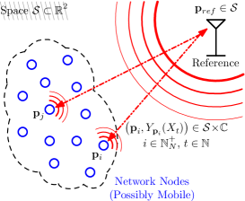
Figure 1: The wireless network of interest.

As already mentioned, the channel state encompasses statistics of the communication medium, and is here modeled as a multidimensional discrete time stochastic process, evolving in time according to a known statistical model. The channel state is assumed to be hidden from the network nodes; the nodes can observe their respective channel realizations, but they cannot directly observe the characteristics of the mechanism that generates these realizations. Naturally, this stochastic structure gives rise to the description of the channel state and the associated observation process(es) as a partially observable stochastic dynamical system.

Let us describe our problem in more explicit mathematical terms. All stochastic processes are defined on a common probability triplet $\left(\Omega,\mathscr{F},{\cal P}\right)$. Let $X_{t}\equiv X_{t}\left(\omega\right)\subset\mathbb{R}^{M\times 1}$, $t\in\mathbb{N}$, $\omega\in\Omega$ denote the hidden channel state. Under the flat fading assumption, the relative to the reference antenna complex channel process at each network node $i\in\mathbb{N}_{N}^{+}$, located at ${\bf p}_{i}\equiv{\bf p}_{i}\left(t\right)\in{\cal S}$ (that is, the nodes might be moving), can be decomposed as [27]

$$\mathbb{C} \ni Y_{i}\left({\bf p}_{i}\left(t\right),X_{t}\right)\equiv Y_{{\bf p}_{i}}\left(X_{t}\right)\equiv\underbrace{Y_{{\bf p}_{i}}^{PL}\left(X_{t}\right)}_{\text{path loss}}\underbrace{Y_{i}^{SH}\left(X_{t}\right)}_{\text{shadowing}}\underbrace{Y_{{\bf p}_{i}}^{MF}\left(t\right)\exp\left(\mathfrak{J}\dfrac{2\pi d_{i}\left(t\right)}{\lambda}\right)}_{\text{fading}},$$ (1)

where $\mathfrak{J}\triangleq\sqrt{-1}$, $\lambda\in\mathbb{R}_{++}$ denotes the wavelength employed for the communication and where: 1) $Y_{{\bf p}_{i}}^{PL}\left(X_{t}\right)\in\mathbb{R}$ denotes path loss, defined as $Y_{{\bf p}_{i}}^{PL}\left(X_{t}\right)\triangleq\left\|{\bf p}_{i}\left(t\right)-{\bf p}_{ref}\right\|_{2}^{-\mu\left(X_{t}\right)/2}\triangleq\left(d_{i}\left(t\right)\right)^{-\mu\left(X_{t}\right)/2}$, where $\mu\left(X_{t}\right)\in\mathbb{R}_{++}$ is the state dependent path loss exponent, which is the same for all network nodes and ${\bf p}_{ref}\in{\cal S}$ denotes the position of the reference antenna in ${\cal S}$. 2) $Y_{i}^{SH}\left(X_{t}\right)\in\mathbb{R}$ denotes the shadowing part of the channel model and its square, conditionally on $X_{t}$, constitutes a base-$10$ log-normal random variable with zero location and scale depending on $X_{t}$. 3) $Y_{{\bf p}_{i}}^{MF}\left(t\right)\in\mathbb{C}$ represents multipath fading, which, for simplicity, is assumed to be a spatiotemporally white, strictly stationary process with fully known statistical description, not associated with $X_{t}$, therefore being an unpredictable complex “observation noise”. Making the substitution $Y_{i}\left({\bf p}_{i}\left(t\right),X_{t}\right)\leftarrow$$\exp\left(-\mathfrak{J}2\pi d_{i}\left(t\right)/\lambda\right)$$Y_{i}\left({\bf p}_{i}\left(t\right),X_{t}\right)$ and using properties of the complex logarithm, we can define the observations of the $i$-th node in logarithmic scale as

$$y_{t}^{i}\triangleq 10\log_{10}\left|Y_{{\bf p}_{i}}\left(X_{t}\right)\right|^{2}-10\mathbb{E}\left\{\log_{10}\left|Y_{{\bf p}_{i}}^{MF}\left(t\right)\right|^{2}\right\}=\\ -10\mu\left(X_{t}\right)\log_{10}\left(d_{i}\left(t\right)\right)+10\log_{10}\left(Y_{i}^{SH}\left(X_{t}\right)\right)^{2}+\\ +\overline{10\log_{10}\left|Y_{{\bf p}_{i}}^{MF}\left(t\right)\right|^{2}}\triangleq\alpha_{t}^{i}\mu\left(X_{t}\right)+\sigma_{t}^{i}\left(X_{t}\right)+\xi_{t}^{i},$$ (2)

where $\overline{\left(\cdot\right)}$ denotes the zero mean version of a random variable. We should emphasize here that by “measurement” or “observation” we refer to the predictable component of the channel, which is described in terms of the channel magnitude.

In similar fashion as in [25], the following further assumptions are made: $\xi_{t}^{i}\overset{i.i.d.}{\sim}{\cal N}\left(0,\sigma_{\xi}^{2}\right),$ $\forall i\in\mathbb{N}_{N}^{+}$ and $\forall t\in\mathbb{N}$. This is a simplified, although quite reasonable assumption. Also see [28]. Second, conditional on $X_{t}$, $\sigma_{t}^{i}\left(X_{t}\right)\overset{i.d.}{\sim}{\cal N}\left(0,\eta^{2}\left(X_{t}\right)\right),\forall i\in\mathbb{N}_{N}^{+}$. This stems from the fact that $\left(Y_{i}^{SH}\left(X_{t}\right)\right)^{2}$ is (base-$10$) log-normally distributed. Additionally, for each set of positions of the network nodes in ${\cal S}$, it is assumed that the members of the set $\left\{\sigma_{t}^{i}\left(X_{t}\right)\right\}_{i\in\mathbb{N}_{N}^{+}}$ constitute jointly normal, spatially correlated random variables with (symmetric and positive definite in $\left({\bf p}_{i}\left(t\right),{\bf p}_{j}\left(t\right)\right)$) conditional on $X_{t}$ autocorrelation kernel

$${\cal R}\left({\bf p}_{i}\left(t\right),{\bf p}_{j}\left(t\right),\boldsymbol{\theta}\left(X_{t}\right)\right):\left({\cal S}\times{\cal S}\times\mathbb{R}^{K}\right)\mapsto\mathbb{R},$$ (3)

for $\left(i,j\right)\in\mathbb{N}_{N}^{+}\times\mathbb{N}_{N}^{+}$, where $K$ denotes the dimension of the state dependent parameter vector $\boldsymbol{\theta}\left(X_{t}\right)$, with

$${\cal R}\left({\bf p}_{i}\left(t\right),{\bf p}_{i}\left(t\right),\boldsymbol{\theta}\left(X_{t}\right)\right) \equiv\eta^{2}\left(X_{t}\right),\quad\forall i\in\mathbb{N}_{N}^{+}.$$ (4)

Therefore, the $\left(i.j\right)$-th entry of the time evolving, conditional (on $X_{t}$) covariance matrix of the random vector $\boldsymbol{\sigma}_{t}\left(X_{t}\right)\triangleq\left[\left\{\sigma_{t}^{i}\left(X_{t}\right)\right\}_{i\in\mathbb{N}_{N}^{+}}\right]^{\boldsymbol{T}}\in\mathbb{R}^{N\times 1}$, $\boldsymbol{\Sigma}_{t}\left(\boldsymbol{\theta}\left(X_{t}\right)\right)\equiv\mathbb{E}\left\{\left.\boldsymbol{\sigma}_{t}\left(X_{t}\right)\left(\boldsymbol{\sigma}_{t}\left(X_{t}\right)\right)^{\boldsymbol{T}}\right|X_{t}\right\}$ $\in{\cal D}_{\boldsymbol{\Sigma}}\subset\mathbb{R}^{N\times N}$, with ${\cal D}_{\boldsymbol{\Sigma}}$ bounded, is defined as

$$\boldsymbol{\Sigma}_{t}\left(\boldsymbol{\theta}\left(X_{t}\right)\right) \left(i,j\right)\triangleq{\cal R}\left({\bf p}_{i}\left(t\right),{\bf p}_{j}\left(t\right),\boldsymbol{\theta}\left(X_{t}\right)\right),$$ (5)

$\forall\left(i,j\right)\in\mathbb{N}_{N}^{+}\times\mathbb{N}_{N}^{+}$. For instance, for the heat kernel type of autocorrelation function employed in [25] and proposed much earlier in [29], defined as

$${\cal R}\left({\bf p}_{i}\left(t\right),{\bf p}_{j}\left(t\right),\boldsymbol{\theta}\left(X_{t}\right)\right) \triangleq{\cal R}\left(d_{ij}\left(t\right),\boldsymbol{\theta}\left(X_{t}\right)\right)\triangleq\theta_{1}\left(X_{t}\right)\exp\left(-\dfrac{d_{ij}\left(t\right)}{\theta_{2}\left(X_{t}\right)}\right),$$ (6)

where $d_{ij}\left(t\right)\triangleq\left\|{\bf p}_{i}\left(t\right)-{\bf p}_{j}\left(t\right)\right\|_{2}\in\mathbb{R}_{+}$, we make the identifications $\boldsymbol{\theta}\left(X_{t}\right)\triangleq\left[\theta_{1}\left(X_{t}\right)\,\theta_{2}\left(X_{t}\right)\right]^{\boldsymbol{T}}$ with $\theta_{1}\left(X_{t}\right)\equiv\eta^{2}\left(X_{t}\right)$. The first parameter, $\theta_{1}\left(X_{t}\right)$, called the shadowing power, controls the variance of the shadowing part of the channel, whereas the second, $\theta_{1}\left(X_{t}\right)$, called the correlation distance, controls the decay rate of the spatial correlation between the channels for each pair of network nodes. This simple isotropic model will be employed in the numerical simulations presented in Section V.

In order to completely define an overall observation process for all nodes in the network, we may stack the $N$ individual channel processes of (2), resulting in the vector additive observation model

$${\bf y}_{t}\equiv\boldsymbol{\alpha}_{t}\mu\left(X_{t}\right)+\boldsymbol{\sigma}_{t}\left(X_{t}\right)+\boldsymbol{\xi}_{t},\quad\forall t\in\mathbb{N},$$ (7)

where $\boldsymbol{\sigma}_{t}\left(X_{t}\right)$ is defined as above and ${\bf y}_{t}\in\mathbb{R}^{N\times 1}$, $\boldsymbol{\alpha}_{t}\in\mathbb{R}^{N\times 1}$ and $\boldsymbol{\xi}_{t}\in\mathbb{R}^{N\times 1}$ are defined accordingly. The observation process (7) can also be rewritten in the canonical form ${\bf y}_{t}\equiv\boldsymbol{\alpha}_{t}\mu\left(X_{t}\right)+\sqrt{{\bf C}_{t}\left(X_{t}\right)}\boldsymbol{u}_{t},\forall t\in\mathbb{N},$ where $\boldsymbol{u}_{t}\equiv\boldsymbol{u}_{t}\left(\omega\right)$ constitutes a standard Gaussian white noise process and ${\bf C}_{t}\left(X_{t}\right)\triangleq\boldsymbol{\Sigma}_{t}\left(\boldsymbol{\theta}\left(X_{t}\right)\right)+\sigma_{\xi}^{2}{\bf I}_{N\times N}\in{\cal D}_{{\bf C}}$, with ${\cal D}_{{\bf C}}$ obviously bounded.

Let us now concentrate more on the time evolving underlying channel state process $X_{t}\in\mathbb{R}^{M\times 1}$. In this work, we will assume that $X_{t}$ constitutes a Markov process with known but nonlinear and (possibly) nonstationary dynamics, described by a possibly nonstationary stochastic kernel ${\cal K}_{t}:\mathscr{B}\left(\mathbb{R}^{M\times 1}\right)\times\mathbb{R}^{M\times 1}\mapsto\left[0,1\right]$. Also, we will make the generic and realistic assumption that the state is confined to a compact strict subset of $\mathbb{R}^{M\times 1}$, that is, $\forall t\in\mathbb{N},X_{t}\in\left[a,b\right]^{M}\triangleq{\cal Z}\subset\mathbb{R}^{M\times 1}$, almost surely. Depending on the available information, instead of using stochastic kernels, we may alternatively assume the existence of an explicit state transition model expressing the temporal evolution of the state, defined as $X_{t}\triangleq f_{t}\left(X_{t-1},W_{t}\right)\in{\cal Z},\forall t\in\mathbb{N},$ where, for each $t$, $f_{t}:{\cal Z}\times{\cal W}\overset{a.s.}{\mapsto}{\cal Z}$ constitutes a measurable nonlinear state transition mapping with somewhat “favorable” analytical behavior (see below) and $W_{t}\equiv W_{t}\left(\omega\right)\in{\cal W}\subseteq\mathbb{R}^{M_{W}\times 1}$, for $t\in\mathbb{N}$, $\omega\in\Omega$, denotes a (discrete time) white noise process with known measure and state space ${\cal W}$.

From now on, in order to facilitate the presentation and without loss of generality, we will drop the subscript “$t$” both in the stochastic kernels and transition mappings governing $X_{t}$, therefore assuming stationarity of the state. Further, for mathematical simplicity, although there are endless possibilities for defining the state dependent functions $\mu\left(X_{t}\right)$ and $\boldsymbol{\theta}\left(X_{t}\right)$, we will assume that $\mu\left(X_{t}\right)\equiv X_{t}\left(1\right)\in\mathbb{R}$ and $\boldsymbol{\theta}\left(X_{t}\right)\equiv\left[X_{t}\left(2\right)\,\ldots\,X_{t}\left(M\right)\right]^{\boldsymbol{T}}\in\mathbb{R}^{\left(M-1\right)\times 1}$, also in agreement with our intuition. From the previous discussion, it follows that the partially observable system defined above constitutes a HMM and can be equivalently described by the system of stochastic difference equations

$$\begin{array}[]{l}\begin{cases}X_{t}\left|X_{t-1}\right.\sim{\cal K}\left(X_{t}\in\text{d}x\left|X_{t-1}\right.\right)&\text{or}\\ X_{t}\equiv f\left(X_{t-1},W_{t}\right)\end{cases}\\ \,\hskip 8.6pt{\bf y}_{t}\equiv\boldsymbol{A}_{t}X_{t}+\boldsymbol{\sigma}_{t}\left(X_{t}\right)+\boldsymbol{\xi}_{t}\end{array},\enskip\forall t\in\mathbb{N},$$ (8)

where $\boldsymbol{A}_{t}\triangleq\left[\boldsymbol{\alpha}_{t}\>{\bf 0}_{N\times\left(M-1\right)}\right]\in\mathbb{R}^{N\times M}$. In addition to the above and in favor of supporting our analytical arguments presented in subsequent sections, we make the following mild assumptions on the functional structure of the observation process of the HMM described by (8).

Assumption 1: (Continuity & Expansiveness) All members of the functional family $\left\{\boldsymbol{\Sigma}_{t}:{\cal Z}\mapsto{\cal D}_{\boldsymbol{\Sigma}}\right\}_{t\in\mathbb{N}}$ are elementwise uniformly Lipschitz continuous, that is, there exists some universal and bounded constant $K_{\boldsymbol{\Sigma}}\in\mathbb{R}_{+}$, such that, $\forall t\in\mathbb{N}$ and $\forall\left(i,j\right)\in\mathbb{N}_{N}^{+}\times\mathbb{N}_{N}^{+}$,

$$\left|\boldsymbol{\Sigma}_{t}^{ij}\left(\boldsymbol{x}\right)-\boldsymbol{\Sigma}_{t}^{ij}\left(\boldsymbol{y}\right)\right|\leq K_{\boldsymbol{\Sigma}}\left\|\boldsymbol{x}-\boldsymbol{y}\right\|_{1},$$ (9)

$\forall\left(\boldsymbol{x},\boldsymbol{y}\right)\in{\cal Z}\times{\cal Z}$. If $\boldsymbol{x}$ is substituted by the stochastic process $X_{t}\left(\omega\right)$, then all the above statements continue to hold almost surely. Also, it is true that

$$\lambda_{inf}\equiv{\displaystyle\inf_{t\in\mathbb{N}}}\hskip 1.99997pt{\displaystyle\inf_{\boldsymbol{x}\in{\cal Z}}}\hskip 1.99997pt\lambda_{min}\left({\bf C}_{t}\left(\boldsymbol{x}\right)\right)>1,$$ (10)

a requirement which can always be satisfied by appropriate normalization of the observations.

For later reference (Section V), let us note that the isotropic autocorrelation kernel previously defined by (6) can be very easily verified to satisfy the Lipschitz condition of Assumption 1, simply considering the compactness of the state vector.

Remark 1.

The assumption of $X_{t}$ satisfying the (first order) Markov property does not offer only analytical tractability, but also practical feasibility. For example, statistical inference in higher order HMMs suffer from the curse of dimensionality so much that, most of the times, the computational effort required for the implementation of basic state estimators is absolutely prohibitive. On the other hand, our proposed formulation is based on general nonlinear models for describing the statistical behavior of the state, offering far greater flexibility, as well as modeling precision, compared to classical linear difference equations. From another point of view, it is well known that a tremendous amount of real world dynamical systems can be modeled using Markov processes and that, in cases where this is not entirely true, Markov processes usually constitute very good modeling approximations.

Let us now define the problems of interest in this paper in a mathematically precise way. Hereafter, strict optimality will be meant to be in the Minimum Mean Square Sense (MMSE). Also, in the following, the natural filtration generated by the causal observation process ${\bf y}_{t}$ is defined as

$$\left\{\mathscr{Y}_{t}\right\}_{t\in\mathbb{N}}\triangleq\left\{\sigma\left\{\left\{{\bf y}_{i}\right\}_{i\in\mathbb{N}_{t}}\right\}\right\}_{t\in\mathbb{N}},$$ (11)

where $\sigma\left\{A\right\}$ denotes the $\sigma$-algebra generated by the random element $A$.

Problem 1.

(Sequential Channel State Tracking (SCST)) Develop a theoretically grounded, sequential scheme for (approximately) evaluating the strictly optimal filter or $\rho$-step predictor of the channel state $X_{t}$ on the basis of the available channel magnitude observations up to time $t$, given by

$$\widehat{X}_{t+\rho}\triangleq\mathbb{E}\left\{\left.X_{t+\rho}\right|\mathscr{Y}_{t}\right\},\quad\forall t\in\mathbb{N},$$ (12)

where $\rho\geq 0$ constitutes the prediction horizon. The computational complexity of the sequential scheme may not grow as more observations become available.

Problem 2.

(Sequential Spatiotemporal Channel Prediction (SSCP)) Develop a theoretically grounded, sequential scheme for (approximately) evaluating the strictly optimal spatiotemporal predictor of the channel magnitude at position ${\bf q}\in\mathbb{R}^{2}$ and time $t+\rho$ ($\rho\geq 0$ is the prediction horizon) given the available channel magnitude observations up to time $t$, expressed as

$$\widehat{y}_{t+\rho}\left({\bf q}\right)\triangleq\mathbb{E}\left\{\left.y_{t+\rho}\left({\bf q}\right)\right|\mathscr{Y}_{t}\right\},\quad\forall t\in\mathbb{N}.$$ (13)

Again, the computational complexity of the sequential scheme may not grow as more observations become available.

Remark 2.

The SSCP problem is clearly related to the channel predictability framework of [25]. In fact, in this paper, we use almost the same channel description (observation process). However, our proposed framework is philosophically different and potentially more general than that proposed in [25], since the underlying channel dynamics (the channel state) are time varying and the considered estimation and prediction problems are formulated in a Bayesian sense.

As we will see in later in Section IV, the SSCP problem can be solved sequentially using the respective sequential solution of the SCST problem. However, unfortunately, it is well known that, except for some very special cases such as those where the state process $X_{t}$ satisfies a linear recursion or where it constitutes a Markov chain (discrete state space) [30, 31, 32, 33], the respective nonlinear filtering and prediction problems do not admit any known sequential (in particular, recursive) representation [34, 26]. Therefore, in order to solve the SCST problem defined above, one typically has to rely on carefully designed and robust approximations to the problem of nonlinear filtering of Markov processes in discrete time, focusing on the class of systems (HMMs) described by (8). This is exactly the subject of the next section.

III Asymptotically Optimal Recursive Filtering & Prediction of Markov Processes: Prior Results & Preliminaries

In the following, we present a number of important results in asymptotically optimal, approximate recursive filtering of Markov processes, recently presented in [35]. These results will provide us with the required mathematical tools for attacking the SCST and SSCP problems, defined previously in Section II.

III-A Uniform State Quantizations

From Section II, we have assumed that $X_{t}\in{\cal Z}\equiv\left[a,b\right]^{M},\forall t\in\mathbb{N},a.s.,$ where, geometrically, ${\cal Z}$ constitutes an $M$-hypercube, representing the compact set of support of the state $X_{t}$. Let us discretize ${\cal Z}$ into $L_{S}\triangleq L^{M}$ hypercubic $M$-dimensional cells of identical volume (each dimension is partitioned in to $L$ intervals). The center of mass of the $l$-th cell is denoted as $\boldsymbol{x}_{L_{S}}^{l},l\in\mathbb{N}_{L_{S}}^{+}$. Then, letting ${\cal X}_{L_{S}}\triangleq\left\{\boldsymbol{x}_{L_{S}}^{l}\right\}_{l\in\mathbb{N}_{L_{S}}^{+}}$, the quantizer ${\cal Q}_{L_{S}}:\left({\cal Z},\mathscr{B}\left({\cal Z}\right)\right)\mapsto\left({\cal X}_{L_{S}},2^{{\cal X}_{L_{S}}}\right)$ is defined as the bijective and measurable function which uniquely maps the $l$-th cell to the respective reconstruction point $\boldsymbol{x}_{L_{S}}^{l}$, $\forall l\in\mathbb{N}_{L_{S}}^{+}$, according to some predefined ordering. That is, ${\cal Q}_{L_{S}}\left(\boldsymbol{x}\right)\triangleq\boldsymbol{x}_{L_{S}}^{l}$ if and only if $\boldsymbol{x}$ belongs to the respective cell (for a detailed and more formalistic definition, see [35]). Having defined the quantizer ${\cal Q}_{L_{S}}\left(\cdot\right)$, we consider the following discrete state space approximations of the process $X_{t}$ [36]:

• The Markovian Quantization of the state, defined as

  $$\widetilde{X}_{t}^{L_{S}}\triangleq{\cal Q}_{L_{S}}\left(f\left(\widetilde{X}_{t-1}^{L_{S}},W_{t}\right)\right)\in{\cal X}_{L_{S}},\quad\forall t\in\mathbb{N}.$$ (14)

  where we have assumed explicitly apriori knowledge of a transition mapping, modeling the temporal evolution of the Markov process $X_{t}$, and

• The Marginal Quantization of the state, defined as

  $$\overline{X}_{t}^{L_{S}}\triangleq{\cal Q}_{L_{S}}\left(X_{t}\right)\in{\cal X}_{L_{S}},\quad\forall t\in\mathbb{N}.$$ (15)

Additionally, for later reference, define the column stochastic matrices $\widetilde{\boldsymbol{P}}\in\left[0,1\right]^{L_{S}\times L_{S}}$ and $\overline{\boldsymbol{P}}\in\left[0,1\right]^{L_{S}\times L_{S}}$ as

$$\widetilde{\boldsymbol{P}}\left(i,j\right) \triangleq{\cal P}\left(\left.\widetilde{X}_{t}^{L_{S}}\equiv\boldsymbol{x}_{L_{S}}^{i}\right|\widetilde{X}_{t-1}^{L_{S}}\equiv\boldsymbol{x}_{L_{S}}^{j}\right)\quad\text{and}$$ (16)

$$\overline{\boldsymbol{P}}\left(i,j\right) \triangleq{\cal P}\left(\left.\overline{X}_{t}^{L_{S}}\equiv\boldsymbol{x}_{L_{S}}^{i}\right|\overline{X}_{t-1}^{L_{S}}\equiv\boldsymbol{x}_{L_{S}}^{j}\right),$$ (17)

$\forall\left(i,j\right)\in\mathbb{N}_{L_{S}}^{+}\times\mathbb{N}_{L_{S}}^{+}$, obviously related to the Markovian and marginal state quantizations, respectively. Due to its structure, $\widetilde{\boldsymbol{P}}$ can at least be constructed simulating $\widetilde{X}_{t}^{L_{S}}$. From the Law of Large Numbers, the entries of $\widetilde{\boldsymbol{P}}$ can be estimated with arbitrary precision from a sufficiently large number of realizations of $\widetilde{X}_{t}^{L_{S}},t\in\mathbb{N}_{T}$, for some $T<\infty$. Similarly, $\overline{\boldsymbol{P}}$ can be estimated also with arbitrary precision from multiple realizations of $\overline{X}_{t}^{L_{S}}$, which constitute a deterministic functional of the true state $X_{t}$. Note, however, that in this case, it is possible to obtain $\overline{\boldsymbol{P}}$ only using available realizations of the state, without actually knowing either the stochastic kernel or the transition mapping of $X_{t}$ (if such exists). For example, this could be made possible in sufficiently controlled physical experiments, specially designed for system identification, where the state $X_{t}$ wou ld be a fully observable stochastic process.

III-B Asymptotically Optimal Recursive Estimators

First, let us introduce the concept of conditional regularity of stochastic kernels and stochastic processes, which, as we will see below, plays an important role in the asymptotic consistency of a special class of approximate state estimators, based on the marginal state quantization discussed above.

Definition 1.

(Conditional Regularity of Stochastic Kernels [35]) Consider the stochastic (or Markov) kernel ${\cal K}:\mathscr{B}\left(\mathbb{R}^{M\times 1}\right)\times\mathbb{R}^{M\times 1}\mapsto\left[0,1\right]$, associated with the process $Y_{t}\left(\omega\right)\in\mathbb{R}^{M\times 1}$, for all $t\in\mathbb{N}$. We say that ${\cal K}\left(\left.\cdot\right|\cdot\right)$ is Conditionally Regular of Type I (CRT I), if, for almost all $\boldsymbol{x}\in{\cal Z}$, there exists a bounded sequence $\delta_{n}\left(\boldsymbol{x}\right)\in\mathbb{R}_{+},n\in\mathbb{N}^{+}$ such that, for ${\cal A}\in\left\{{\cal Z}_{L_{S}}^{j}\right\}_{j\in\mathbb{N}_{L_{S}}^{+}}$,

$$\begin{array}[]{c}{\displaystyle\sup_{{\cal A}}}\left|{\cal K}\left(\left.{\cal A}\right|\boldsymbol{x}\right)-{\cal K}\left({\cal A}\left|{\cal Q}_{L_{S}}\left(\boldsymbol{x}\right)\right.\right)\right|\leq\dfrac{\delta_{L_{S}}\left(\boldsymbol{x}\right)}{L_{S}}\\ \text{with}\quad{\displaystyle\lim_{L_{S}\rightarrow\infty}}\delta_{L_{S}}\left(\boldsymbol{x}\right)\equiv 0,\quad a.e.\end{array},$$ (18)

If, additionally, for almost all $\boldsymbol{x}\in\mathbb{R}^{M\times 1}$, the Borel probability measure ${\cal K}\left(\left.\cdot\right|\boldsymbol{x}\right)$ admits a stochastic kernel density $\kappa:\mathbb{R}^{M\times 1}\times\mathbb{R}^{M\times 1}\mapsto\left[0,1\right],$ suggestively denoted as $\kappa\left(\left.\boldsymbol{y}\right|\boldsymbol{x}\right)$ and if the condition

$$\begin{array}[]{c}{\displaystyle\sup_{\boldsymbol{y}\in\mathbb{R}^{M\times 1}}}\left|\kappa\left(\left.\boldsymbol{y}\right|\boldsymbol{x}\right)-\kappa\left(\left.\boldsymbol{y}\right|{\cal Q}_{L_{S}}\left(\boldsymbol{x}\right)\right)\right|\leq\delta_{L_{S}}\left(\boldsymbol{x}\right)\\ \text{with}\quad{\displaystyle\lim_{L_{S}\rightarrow\infty}}\delta_{L_{S}}\left(\boldsymbol{x}\right)\equiv 0,\quad a.e.\end{array},$$ (19)

is satisfied, then we say that ${\cal K}\left(\left.\cdot\right|\cdot\right)$ is Conditionally Regular of Type II (CRT II). In any of the two cases, we will also say that $Y_{t}$ is conditionally regular, interchangeably.

 

We are now ready to present the following two central results, establishing that, under Assumption 1 and certain but mild assumptions on the nature of the state process $X_{t}$, it is possible to approximate the strictly optimal nonlinear filter/predictor $\widehat{X}_{t+\rho}$ by a simple recursive filtering scheme, being formally similar to the MMSE optimal filter of a Markov chain with finite state space. The resulting approximate filter is strongly theoretically consistent, in the sense that it converges to the true optimal filter of the state uniformly inside each fixed finite time interval and uniformly in a measurable set consisting of possible outcomes occurring with probability almost $1$.

The results are presented below. The proofs are omitted, since each one of them essentially constitutes a fusion of several related results recently presented by the authors in [35]. In the following, ${\cal Q}_{L_{S}}^{e}:\left({\cal X}_{L_{S}},2^{{\cal X}_{L_{S}}}\right)\mapsto\left({\cal B}_{L_{S}},2^{{\cal B}_{L_{S}}}\right)$ constitutes a unique bijective mapping between the sets ${\cal X}_{L_{S}}$ and ${\cal B}_{L_{S}}\triangleq\left\{{\bf e}_{l}^{L_{S}}\right\}_{l\in\mathbb{N}_{L_{S}}^{+}}$, where the latter contains as elements the complete standard basis in $\mathbb{R}^{L_{S}\times 1}$.

Theorem 1.

(Approximate Filtering of Markov Processes [35]) Define the reconstruction and likelihood matrices as

$${\bf X} \triangleq\left[\boldsymbol{x}_{L_{S}}^{1}\,\boldsymbol{x}_{L_{S}}^{2}\,\ldots\,\boldsymbol{x}_{L_{S}}^{L_{S}}\right]\in\mathbb{R}^{M\times L_{S}}\quad\text{and}$$ (20)

$$\boldsymbol{\Lambda}_{t} \triangleq\mathrm{diag}\left(\left\{\lambda_{t}\left(\boldsymbol{x}_{L_{S}}^{j}\right)\right\}_{j\in\mathbb{N}_{L_{S}}^{+}}\right)\in\mathbb{R}^{L_{S}\times L_{S}},$$ (21)

respectively, where, for all $t\in\mathbb{N}$, $\lambda_{t}\left(\boldsymbol{x}_{L_{S}}^{j}\right)$ is given by (24) (top of next page). Then, the strictly optimal filter and $\rho$-step predictor of the state process $X_{t}$ can be approximated as

$${\cal E}^{L_{S}}\left(\left.X_{t+\rho}\right|\mathscr{Y}_{t}\right)\triangleq\dfrac{{\bf X}\boldsymbol{P}^{\rho}E_{t}}{\left\|E_{t}\right\|_{1}},\quad\forall t\in\mathbb{N}$$ (22)

and for all finite prediction horizons $\rho\geq 0$, where the process $E_{t}\in\mathbb{R}^{L_{S}\times 1}$ on the RHS of (22) satisfies the simple linear recursion

$$E_{t}\equiv\boldsymbol{\Lambda}_{t}\boldsymbol{P}E_{t-1},\quad\forall t\in\mathbb{N}$$ (23)

and where

• $\boldsymbol{P}\equiv\widetilde{\boldsymbol{P}}$, for the Markovian quantization of the state and

• $\boldsymbol{P}\equiv\overline{\boldsymbol{P}}$, for the marginal quantization of the state.

The approximate filter ${\cal E}^{L_{S}}\left(\left.X_{t}\right|\mathscr{Y}_{t}\right)$ is initialized at time $t\equiv-1$ setting $E_{-1}\equiv\mathbb{E}\left\{{\cal Q}_{L_{S}}^{e}\left(\widetilde{X}_{-1}^{L_{S}}\right)\right\}$ for the Markovian quantization and $E_{-1}\equiv\mathbb{E}\left\{{\cal Q}_{L_{S}}^{e}\left(\overline{X}_{-1}^{L_{S}}\right)\right\}$ for the marginal quantization of the state.

$$\lambda_{t}\left(\boldsymbol{x}_{L_{S}}^{j}\right)\triangleq\dfrac{\exp\left(-\dfrac{1}{2}\left({\bf y}_{t}-\boldsymbol{A}_{t}\boldsymbol{x}_{L_{S}}^{j}\right)^{\boldsymbol{T}}\left(\boldsymbol{\Sigma}_{t}\left(\boldsymbol{x}_{L_{S}}^{j}\right)+\sigma_{\xi}^{2}{\bf I}_{N\times N}\right)^{-1}\left({\bf y}_{t}-\boldsymbol{A}_{t}\boldsymbol{x}_{L_{S}}^{j}\right)\right)}{\sqrt{\det\left(\boldsymbol{\Sigma}_{t}\left(\boldsymbol{x}_{L_{S}}^{j}\right)+\sigma_{\xi}^{2}{\bf I}_{N\times N}\right)}},$$ (24)

Theorem 2.

(Asymptotic Optimality of Approximate Filters [35]) Pick any natural $T<\infty$ and suppose either of the following:

• The Markovian quantization is employed, whose initial value coincides with that of $X_{t}$, and the transition mapping of the state, $f:{\cal Z}\times{\cal W}\overset{a.s.}{\mapsto}{\cal Z}$, is Lipschitz in ${\cal Z}$, for every element of ${\cal W}$.

• The marginal quantization is employed and $X_{t}$ is conditionally regular.

Then, for any finite prediction horizon $\rho\geq 0$, there exists a measurable subset $\widehat{\Omega}_{T}\subseteq\Omega$ with ${\cal P}$-measure at least $1-\left(T+1\right)^{1-CN}\exp\left(-CN\right)$, such that

$$\sup_{t\in\mathbb{N}_{T}}\sup_{\omega\in\widehat{\Omega}_{T}}\left\|{\cal E}^{L_{S}}\left(\left.X_{t+\rho}\right|\mathscr{Y}_{t}\right)-\widehat{X}_{t+\rho}\right\|_{1}\underset{L_{S}\rightarrow\infty}{\longrightarrow}0,$$ (25)

for any free, finite constant $C\geq 1$. In other words, the convergence of the respective approximate filters is compact in $t\in\mathbb{N}$ and, with probability at least $1-\left(T+1\right)^{1-CN}\exp\left(-CN\right)$, uniform in $\omega$.

Note that while the approximate filters/predictors described in Theorem 1 are structurally very simple, they converge to the respective optimal nonlinear state estimators in a particularly strong sense (under the respective conditions), as Theorem 2 clearly suggests.

IV SCST & SSCP in Mobile Wireless Networks

In this section, we present the main results of the paper. In a nutshell, we propose two theoretically consistent sequential algorithms for approximately solving the SCST and SSCP problems defined in Section II.B, both derived as applications of Theorem 1, presented in Section III.

IV-A SCST

At this point, it is apparent that Theorem 1 in fact directly provides us with an effective approximate and recursive estimator for the channel state $X_{t}$. Therefore, Theorem 1 immediately solves the SCST problem, since the resulting filtering/prediction scheme is sequential and, as new channel measurements become available, its computational complexity is fixed, due to time invariance of the type of numerical operations required for each filter update.

Specifically, Algorithm 1 shows the discrete steps required for the centralized implementation of the proposed filtering scheme, in a relatively powerful fusion center. Observe that, depending on the type of quantization employed and for each $\rho\geq 0$, the required matrices $\boldsymbol{P}$ and ${\bf X}\boldsymbol{P}^{\rho}$ can be computed offline and stored in memory.

1. Choose $\boldsymbol{P}$ and $E_{-1}$ depending on the type of state quantization employed (Markovian or marginal).

2. Choose $\rho\geq 0$ and recall $\boldsymbol{P}$ and ${\bf X}\boldsymbol{P}^{\rho}$ from memory.

3. For $t=0,1,...$ do

4. Compute the diagonal matrix $\boldsymbol{\Lambda}_{t}$ from (24).

5. Compute & store

   $$E_{t}=\boldsymbol{\Lambda}_{t}\boldsymbol{P}E_{t-1},$$

   until the next iteration.

6. Normalize $E_{t}$ as

   $$E_{t}^{N}=\dfrac{E_{t}}{\left\|E_{t}\right\|_{1}}.$$

7. Compute & output $E_{t}$ as

   $${\cal E}^{L_{S}}\left(\left.X_{t+\rho}\right|\mathscr{Y}_{t}\right)={\bf X}\boldsymbol{P}^{\rho}E_{t}^{N}.$$

8. endFor

Algorithm 1 Sequential Channel State Tracking

IV-B SSCP

Defining the natural filtration generated by both the state $X_{t}$ and the observations ${\bf y}_{t}$ as

$$\left\{\mathscr{H}_{t}\right\}_{t\in\mathbb{N}}\triangleq\left\{\sigma\left\{\left\{X_{t},{\bf y}_{i}\right\}_{i\in\mathbb{N}_{t}}\right\}\right\}_{t\in\mathbb{N}}$$ (26)

and using the tower property of expectations, it is true that

$$\widehat{y}_{t}\left({\bf q}\right) \equiv\mathbb{E}\left\{\left.y_{t}\left({\bf q}\right)\right|\mathscr{Y}_{t}\right\}$$

$$\equiv\mathbb{E}\left\{\left.\mathbb{E}\left\{\left.y_{t}\left({\bf q}\right)\right|\mathscr{H}_{t}\right\}\right|\mathscr{Y}_{t}\right\},\quad\forall t\in\mathbb{N}.$$ (27)

Let us define the quantities

$$\alpha^{{\bf q}} \triangleq-10\log_{10}\left(\left\|{\bf q}-{\bf p}_{ref}\right\|_{2}\right),$$ (28)

$$\left.\sigma^{{\bf q}}\left(X_{t}\right)\right|X_{t} \overset{def}{\sim}{\cal N}\left(0,\eta^{2}\left(X_{t}\right)\right)\quad\text{and}$$ (29)

$$\xi^{{\bf q}} \overset{def}{\sim}{\cal N}\left(0,\sigma_{\xi}^{2}\right),$$ (30)

where, also by definition,

$$\mathbb{E}\left\{\left.\begin{bmatrix}\boldsymbol{\sigma}_{t}\left(X_{t}\right)\\ \sigma^{{\bf q}}\left(X_{t}\right)\end{bmatrix}\begin{bmatrix}\boldsymbol{\sigma}_{t}\left(X_{t}\right)\\ \sigma^{{\bf q}}\left(X_{t}\right)\end{bmatrix}^{\boldsymbol{T}}\right|X_{t}\right\} \triangleq\begin{bmatrix}\boldsymbol{\Sigma}_{t}\left(X_{t}\right)&\boldsymbol{\sigma}_{t}^{{\bf q}}\left(X_{t}\right)\\ \left(\boldsymbol{\sigma}_{t}^{{\bf q}}\left(X_{t}\right)\right)^{\boldsymbol{T}}&\eta^{2}\left(X_{t}\right)\end{bmatrix},$$ (31)

with each element of $\boldsymbol{\sigma}_{t}^{{\bf q}}\left(X_{t}\right)\in\mathbb{R}^{N\times 1}$ given by

$$\boldsymbol{\sigma}_{t}^{{\bf q}}\left(X_{t}\right)\left(j\right)\triangleq{\cal{\cal R}}\left({\bf q},{\bf p}_{j}\left(t\right),\boldsymbol{\theta}\left(X_{t}\right)\right),\quad\forall j\in\mathbb{N}_{N}^{+}.$$ (32)

Then, it must be true that

$$y_{t}\left({\bf q}\right) \equiv\alpha^{{\bf q}}X_{t}\left(1\right)+\sigma^{{\bf q}}\left(X_{t}\right)+\xi^{{\bf q}}$$

$$\equiv A^{{\bf q}}X_{t}+\sigma^{{\bf q}}\left(X_{t}\right)+\xi^{{\bf q}},$$ (33)

where $A^{{\bf q}}\triangleq\left[\alpha^{{\bf q}}\,{\bf 0}_{1\times\left(M-1\right)}\right]\in\mathbb{R}^{1\times M}$, since $y_{t}\left({\bf q}\right)$ can be equivalently considered as an additional observation, measured by an imaginary sensor at position ${\bf q}$, which of course was not used for state estimation in the SCST problem treated above. Under these considerations, the inner conditional expectation of (27) can be expressed as

$$\mathbb{E}\left\{\left.y_{t}\left({\bf q}\right)\right|\mathscr{H}_{t}\right\} \equiv\mathbb{E}\left\{\left.A^{{\bf q}}X_{t}+\sigma^{{\bf q}}\left(X_{t}\right)+\xi^{{\bf q}}\right|\mathscr{H}_{t}\right\}$$

$$\equiv A^{{\bf q}}X_{t}+\mathbb{E}\left\{\left.\sigma^{{\bf q}}\left(X_{t}\right)\right|\mathscr{H}_{t}\right\},$$ (34)

or, using well known properties of jointly Gaussian random vectors [37] (also used in [25]),

$$\mathbb{E}\left\{\left.y_{t}\left({\bf q}\right)\right|\mathscr{H}_{t}\right\} =A^{{\bf q}}X_{t}+\left(\boldsymbol{\sigma}_{t}^{{\bf q}}\left(X_{t}\right)\right)^{\boldsymbol{T}}{\bf C}_{t}^{-1}\left(X_{t}\right)\left({\bf y}_{t}-\boldsymbol{A}_{t}X_{t}\right)\triangleq\phi_{t}\left(X_{t},{\bf y}_{t}\right).$$ (35)

As a result, $\widehat{y}_{t}\left({\bf q}\right)$ can be expressed as

$$\widehat{y}_{t}\left({\bf q}\right)\equiv\mathbb{E}\left\{\left.\phi_{t}\left(X_{t},{\bf y}_{t}\right)\right|\mathscr{Y}_{t}\right\},$$ (36)

that is, the SSCP problem coincides with the problem of sequentially evaluating the optimal nonlinear filter of a particular functional of the state and the observations, $\phi_{t}\left(\cdot,\cdot\right)$. In this respect, the following result is true, which, together with the results presented in Section III, has also been formulated previously by the authors in [35].

Theorem 3.

(Approximate Filtering for Functionals of the State / Separation Theorem [35]) For any deterministic functional family $\left\{\boldsymbol{\phi}_{t}:\mathbb{R}^{L_{S}\times 1}\mapsto\mathbb{R}^{M_{\phi_{t}}\times 1}\right\}_{t\in\mathbb{N}}$ with bounded and continuous members and any finite prediction horizon $\rho\geq 0$, the strictly optimal filter and $\rho$-step predictor of the transformed process $\boldsymbol{\phi}_{t}\left(X_{t}\right)$ can be approximated as

$${\cal E}^{L_{S}}\left(\left.\boldsymbol{\phi}_{t+\rho}\left(X_{t+\rho}\right)\right|\mathscr{Y}_{t}\right)\triangleq\boldsymbol{\Phi}_{t+\rho}\dfrac{\boldsymbol{P}^{\rho}E_{t}}{\left\|E_{t}\right\|_{1}}\in\mathbb{R}^{M_{\phi_{t}}\times 1},$$ (37)

for all $t\in\mathbb{N}$, where the process $E_{t}\in\mathbb{R}^{L_{S}\times 1}$ can be recursively evaluated as in Theorem 1 and

$$\boldsymbol{\Phi}_{t+\rho}\triangleq\left[\boldsymbol{\phi}_{t+\rho}\left(\boldsymbol{x}_{L_{S}}^{1}\right)\,\ldots\,\boldsymbol{\phi}_{t+\rho}\left(\boldsymbol{x}_{L_{S}}^{L_{S}}\right)\right]\in\mathbb{R}^{M_{\phi_{t}}\times L_{S}}.$$ (38)

In the above, the transition matrix $\boldsymbol{P}$ and the initialization of the approximate filter are exactly the same as in Theorem 1. Additionally, the approximate filter is asymptotically optimal under the same conditions and in the same sense as in Theorem 2.

Invoking Theorem 3, the following result is true, providing a closed form approximate solution to the SSCP problem, at the same time enjoying asymptotic optimality in the sense of Theorem 2.

Theorem 4.

(Approximate Solution to the SSCP Problem) The strictly optimal spatiotemporal predictor of the channel magnitude at an arbitrary position ${\bf q}\in\mathbb{R}^{2}$, $\widehat{y}_{t}\left({\bf q}\right)$, can be approximated as

$${\cal E}^{L_{S}}\left(\left.y_{t+\rho}\left({\bf q}\right)\right|\mathscr{Y}_{t}\right)\triangleq\begin{cases}{\displaystyle\left\langle\boldsymbol{\phi}_{t}\left({\bf y}_{t}\right),\dfrac{E_{t}}{\left\|E_{t}\right\|_{1}}\right\rangle},&\rho\equiv 0\\ A^{{\bf q}}{\bf X}\boldsymbol{P}^{\rho}\dfrac{E_{t}}{\left\|E_{t}\right\|_{1}},&\rho\geq 1\end{cases},$$ (39)

for all $t\in\mathbb{N}$, where the process $E_{t}\in\mathbb{R}^{L_{S}\times 1}$ can be recursively evaluated as in Theorem 1 and where the stochastic process $\boldsymbol{\phi}_{t}\left({\bf y}_{t}\right)\in\mathbb{R}^{L_{S}\times 1}$ is defined as

$$\boldsymbol{\phi}_{t}\left({\bf y}_{t}\right)\triangleq\left[\phi_{t}\left(\boldsymbol{x}_{L_{S}}^{1},{\bf y}_{t}\right)\,\ldots\,\phi_{t}\left(\boldsymbol{x}_{L_{S}}^{L_{S}},{\bf y}_{t}\right)\right]^{\boldsymbol{T}},$$ (40)

with $\phi_{t}:\mathbb{R}^{M\times 1}\times\mathbb{R}^{N\times 1}\mapsto\mathbb{R}$ defined as in (35). In the above, the transition matrix $\boldsymbol{P}$ and the initialization of the approximate filter are exactly the same as in Theorem 1. Additionally, under the same conditions as in Theorem 2, it is true that

$$\sup_{t\in\mathbb{N}_{T}}\sup_{\omega\in\widehat{\Omega}_{T}}\left|{\cal E}^{L_{S}}\left(\left.y_{t+\rho}\left({\bf q}\right)\right|\mathscr{Y}_{t}\right)-\widehat{y}_{t+\rho}\left({\bf q}\right)\right|\underset{L_{S}\rightarrow\infty}{\longrightarrow}0.$$ (41)

1. Choose $\boldsymbol{P}$ and $E_{-1}$ depending on the type of state quantization employed (Markovian or marginal).

2. Choose $\rho\geq 0$ and recall $\boldsymbol{P}$ and ${\bf X}\boldsymbol{P}^{\rho}$ from memory.

3. Choose an arbitrary ${\bf q}\in\mathbb{R}^{2}$.

4. For $t=0,1,...$ do

5. Compute the diagonal matrix $\boldsymbol{\Lambda}_{t}$ from (24).

6. Compute

   $$E_{t}=\boldsymbol{\Lambda}_{t}\boldsymbol{P}E_{t-1},$$

   & store it until the next iteration.

7. Normalize $E_{t}$ as

   $$E_{t}^{N}=\dfrac{E_{t}}{\left\|E_{t}\right\|_{1}}.$$

8. Compute vector $\boldsymbol{\phi}_{t}\left({\bf y}_{t}\right)$ using current observations  from (35) and (40).

9. Compute & output ${\cal E}^{L_{S}}\left(\left.y_{t+\rho}\left({\bf q}\right)\right|\mathscr{Y}_{t}\right)$ as

   $${\cal E}^{L_{S}}\left(\left.y_{t+\rho}\left({\bf q}\right)\right|\mathscr{Y}_{t}\right)\triangleq\begin{cases}{\displaystyle\left\langle\boldsymbol{\phi}_{t}\left({\bf y}_{t}\right),E_{t}^{N}\right\rangle},&\rho\equiv 0\\ A^{{\bf q}}{\bf X}\boldsymbol{P}^{\rho}E_{t}^{N},&\rho\geq 1\end{cases}.$$

10. endFor

Algorithm 2 Sequential Spatiotemporal Channel Prediction

Proof:

See Appendix. ∎

Algorithm 2 shows the discrete steps required for the centralized implementation of the proposed approximate spatial prediction scheme.

IV-C Computational Complexity: A Fair Comparison

A careful inspection of Algorithms 1 and 2 proposed earlier for the solution of the SCST and SSCP problems, respectively, reveals that, in the worst case, the computational complexity of both algorithms scales as ${\cal O}\left(L_{S}^{2}+L_{S}N^{3}\right)$. The two algorithms can also be combined into one with the same computational requirements. The cubic term related to the number of sensors in the network is due to the inversion and the determinant calculation of the covariance matrices, for each reconstruction point $\boldsymbol{x}_{L_{S}}^{j},j\in\mathbb{N}_{L_{S}}^{+}$ and at each time instant $t\in\mathbb{N}$, and it is computationally bearable, at least for a relatively small number of sensors. However, note that when the sensors are stationary or even when their trajectories are fixed and known apriori, the aforementioned computationally demanding operations may be completely bypassed by precomputing the required matrices for each set of parameters and storing them in memory. In such a case, the computational complexity of both algorithms reduces significantly to ${\cal O}\left(L_{S}^{2}+L_{S}N^{2}\right)$.

Temporarily considering the number of sensors $N$ as constant and focusing solely on the number of quantization regions $L_{S}$, it is apparent that the complexity of both algorithms considered scales as ${\cal O}\left(L_{S}^{2}\right)$. This can be very large if one considers the same quantization resolution in each dimension of the Euclidean space the state process lives in, that is, as in Section III.A, where, for simplicity, we considered a completely uniform strictly hypercubic quantizer on the set $\left[a,b\right]^{M}$. Specifically, in this general case, where we “pay the same attention” to all points in the $M$-hypercube of interest, the overall complexity scales as ${\cal O}\left(L_{S}^{2}\equiv L^{2M}\right)$, which, of course, is clearly prohibitively large for high dimensional systems. However, as analyzed in [35], no one prevents us from considering either hyperrectangular Euclidean state spaces since, in most cases, each element of the state vector would have its own dynamic range, or different quantization resolution for each element, since they may not have all the same importance in the particular engineering application of interest, or both.

In the particular problems we are interested in here, the dimension of the state process is relatively low, that is, the range of $M$ almost always between 2 and 5 dimensions, which makes grid based filters practically feasible. Additionally, as we will see in Section V, where we present the relevant numerical simulations and as it has already been clearly shown in [25] in a non Bayesian framework, if one considers the simple isotropic autocorrelation kernel described by (6) in Section II.B and is primarily interested in the SSCP problem, the sensitivity of the quality of spatial channel prediction on the estimation error of the shadowing power and decorrelation distance of the channel is indeed very low, making it possible to potentially consider a lower quantization resolution for the aforementioned quantities without significant compromise in terms of the prediction quality. As a result, grid based approximate filters are indeed adequate for the problems of interest in this paper, taking advantage of their strong properties in terms of asymptotic consistency.

Naturally, particle filters [38, 39] would constitute the rivals of our grid based filtering approach. Compared to the former, particle filters exhibit a computational complexity of ${\cal O}\left(L_{S}\right)$, where, in this case, $L_{S}$ constitutes the number of particles [38]. That is, the complexity of particle filters is one order of magnitude smaller compared to the complexity of grid based filters. Note, though, that in Algorithms 1 and 2, the one and only computational operation which incurs a complexity of ${\cal O}\left(L_{S}^{2}\right)$ is the matrix vector operation $\boldsymbol{P}E_{t-1}$. In fact, in the numerical simulations conducted in Section V, it was revealed that, at least for the problems of interest, the numerical operations of inversion and determinant computation of the respective covariance matrices are far more computationally important than the aforementioned matrix vector multiplication. These operations would be also required in a typical particle filter implementation as well.

Continuing the comparison of the proposed approach with the filtering approximation family of particle filters, another issue of major importance is filter behavior with respect to the curse of dimensionality. Although in, for instance, [40] and [41], it was warmly asserted that the use of particle filters might indeed make it possible to beat the curse of dimensionality, it was later made clear that this is not the case and that particle filters indeed suffer from the curse [42, 43, 44]. More recently, it was shown that particle filters suffer in general both in terms of temporal uniformity in the convergence of the respective filtering approximations and in terms of exponential dependence on the dimensionality of the observation process [45] and that of the state process as well [44], greatly affecting rate of convergence. In fact, as also shown in [45], in order to somewhat circumvent these important practical limitations, strict assumptions must hold regarding the structure of the partially observable system under consideration, therefore somewhat limiting the general applicability of the respective methods presented in [45]. Of course, the grid-based filters proposed in this paper suffer from similar drawbacks [35], a fact that strengthens the common belief that, at least in the context of nonlinear filtering, the curse of dimensionality constitutes a ubiquitous phenomenon.

However, from a technical point of view, the grid based filters we propose for effectively solving the SCST and SSCP problems are very consistent, in the sense that their convergence to the true nonlinear filter of the state is compact in time and uniform with respect to a set of possible outcomes of almost full probability measure. Although, due to our inability to show uniform convergence in time (however keeping the class of admissible hidden Markov process large), we cannot theoretically prove that the proposed approximate filters can indeed reach a stable steady state, we can at least guarantee that the approximation error will be uniformly bounded for any fixed time interval set by the user, with overwhelmingly high probability (for more details, see [46] and [35]). Further, as we will see in the next section, the practical performance of the filters, at least when considering the autocorrelation kernel of (6), is very robust and tracks the hidden system accurately, for a relatively small number of quantization cells, without the need of any fine tuning, as opposed to the case of particle filters (choice of importance density, etc.) [38].

V Numerical Simulations

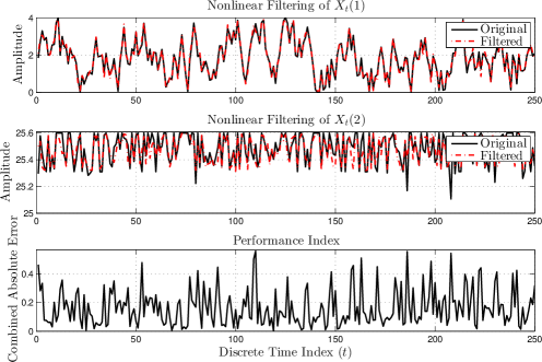
(a)

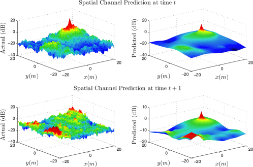
(b)

Figure 2: (a) Demonstration of channel state tracking for 250 time steps. The estimates are produced from the observations of 30 randomly scattered sensors in the square region $\left[-20\,m,20\,m\right]^{2}$. (b) Spatial prediction and temporal tracking of the channel combined. In this example, the spatial grid consists of 3600 evaluation points and the results are obtained using just 30 spatial measurements. Observe how the prediction procedure dynamically captures the basic characteristics of the channel, exploiting the spatial correlations due to shadowing.

The practical effectiveness of Algorithms 1 and 2 will also be validated through a number of sufficiently representative synthetic experiments. Specifically, we consider $N\equiv 30$ sensors randomly scattered on a sufficiently fine square grid, in the square region of the $x/y$ plane ${\cal S}\equiv\left[0,40\right]^{2}$ (in $m\times m$). The position of the reference antenna is fixed at ${\bf p}_{ref}\equiv\left[25\,10\right]^{\boldsymbol{T}}$. Concerning the behavior of the communication channel throughout the plane, the variance of the multipath fading noise term is set at $\sigma_{\xi}^{2}\equiv 2$ and, as far as shadowing is concerned, the autocorrelation kernel of (6) is employed, where, for simplicity, we assume that the correlation distance is known and constant with respect to time and equal to $10\,m$. As a result, in this simple example, the channel state is two dimensional, with $X_{t}\left(1\right)\equiv\mu\left(X_{t}\right)$ and $X_{t}\left(2\right)\equiv\boldsymbol{\theta}\left(X_{t}\right)$ representing the path loss coefficient and the shadowing power, respectively. The temporal evolution of each respective component of the channel state is given by the stochastic difference equations

$$X_{t}\left(1\right) \equiv\tanh\left(\gamma\left(X_{t-1}\left(1\right)-2\right)\right)+W_{t}+2,\quad\text{and}$$ (42)

$$X_{t}\left(2\right) \equiv 0.3\left|\tanh\left(\sin\left(\gamma X_{t-1}\left(2\right)W_{t}\right)\right.\right.+$$

$$\hskip 30.00005pt\left.\left.+X_{t-1}\left(2\right)W_{t}\right)+W_{t}\right|+25,\quad\forall t\in\mathbb{N},$$ (43)

for some arbitrary but known initial conditions, where $\gamma\equiv 1.6$ and $W_{t}\equiv\text{clip}_{\left[-1,1\right]}\left(G_{t}\right)$, $G_{t}\overset{i.i.d.}{\sim}{\cal N}\left(0,1\right)$, with $\text{clip}_{\left[-1,1\right]}\left(\cdot\right)$ denoting the hard limiter operation into the set $\left[-1,1\right]$. Note that both difference equations are strongly nonlinear in in both the state and driving noise. Also note the strong coupling between the two equations, due to the fact that both are driven by exactly the same noise realizations. The above equations attempt to model a situation where the path loss exponent is somewhat slowly varying between $0$ and $4$, whereas the shadowing power is rapidly varying between $25$ and $25.6$. The state $X_{t}\equiv\left[X_{t}\left(1\right)\,X_{t}\left(2\right)\right]^{\boldsymbol{T}}$ was uniformly quantized into $L_{S}\equiv 30^{2}$ cells (that is, $L\equiv 30$). For simplicity, regarding the simulation results which will be presented and discussed below, we focus on the case where $\rho\equiv 0$, that is, we consider the problems of temporal filtering of the channel state and spatial prediction of the channel, which both constitute instances of the SCST and SSCP problems, respectively.

Fig. 2a demonstrates the channel state tracking (temporal filtering of the state) for $250$ time steps, according to the experimental setting stated above. As illustrated in the figure, the quality of the estimates is very good, considering the nonlinearity present both in the state process and the observations at each sensor in the network. It also apparent that the produced estimation process behaves in a stable manner, as time increases.

The filter of the channel state can subsequently be used for the also asymptotically optimal prediction of the channel magnitude in the rest of the space. This is illustrated in Fig. 2b, where the combined spatial prediction and temporal tracking of the channel magnitudes are shown (for two time instants), in comparison to the real channel maps in the square region under consideration. The random field used for modeling the spatial channel process was generated using a spatial grid of $3600$ points and the respective predicted values were obtained from just $N\equiv 30$ random scattered spatial channel measurements in the region of interest. From the figure, it can be seen that the quality of the predicted process is very good, especially considering the fact that the channel is reconstructed using only $0.83\,\%$ of the total number of grid points in the region of interest. Of course, the quality of the spatial prediction improves as the number of spatial measurements (and therefore nodes/sensors) increases. One can observe that the prediction procedure accurately captures the basic characteristics of the channel in the region of interest, effectively exploiting the spatial correlations due to shadowing.

VI Conclusion

In this paper, a nonlinear filtering framework was proposed for addressing the fundamental problems of sequential channel state tracking and spatiotemporal channel prediction in mobile wireless sensor networks. First, we formulated the channel observations at each sensor as a partially observable nonlinear system with temporally varying state and spatiotemporally varying observations. Then, a grid based approximate filtering scheme was employed for accurately tracking the temporal variation of the channel state, based on which we proposed a recursive spatiotemporal channel gain predictor, providing real time sequential CG map estimation at each sensor in the network. Further, we showed that both estimators are asymptotically optimal, in the sense that they converge to the optimal MMSE estimators/predictors of the channel state and observations at unobserved positions in the region of interest, respectively, in a technically strong sense. In addition to these theoretical results, numerical simulations were presented, validating the practical effectiveness of the proposed approach and increasing the user’s confidence for practical consideration in real world wireless networks.

Appendix
Proof of Theorem 4

Let us first consider the filtering case, that is, the one where $\rho\equiv 0$. Substituting (35) to (36), we get

$$\widehat{y}_{t}\left({\bf q}\right)\equiv\mathbb{E}\left\{\left.A^{{\bf q}}X_{t}+\left(\boldsymbol{\sigma}_{t}^{{\bf q}}\left(X_{t}\right)\right)^{\boldsymbol{T}}{\bf C}_{t}^{-1}\left(X_{t}\right)\left({\bf y}_{t}-\boldsymbol{A}_{t}X_{t}\right)\right|\mathscr{Y}_{t}\right\}\\ \equiv A^{{\bf q}}\mathbb{E}\left\{\left.X_{t}\right|\mathscr{Y}_{t}\right\}+\mathbb{E}\left\{\left.\left(\boldsymbol{\sigma}_{t}^{{\bf q}}\left(X_{t}\right)\right)^{\boldsymbol{T}}{\bf C}_{t}^{-1}\left(X_{t}\right)\right|\mathscr{Y}_{t}\right\}{\bf y}_{t}-\\ -\mathbb{E}\left\{\left.\left(\boldsymbol{\sigma}_{t}^{{\bf q}}\left(X_{t}\right)\right)^{\boldsymbol{T}}{\bf C}_{t}^{-1}\left(X_{t}\right)\boldsymbol{A}_{t}X_{t}\right|\mathscr{Y}_{t}\right\},\quad\forall t\in\mathbb{N},$$ (44)

from where, defining the bounded and continuous functionals

$$\boldsymbol{\phi}_{t}^{1}\left(X_{t}\right) \triangleq\left(\left(\boldsymbol{\sigma}_{t}^{{\bf q}}\left(X_{t}\right)\right)^{\boldsymbol{T}}{\bf C}_{t}^{-1}\left(X_{t}\right)\right)^{\boldsymbol{T}}\in\mathbb{R}^{N\times 1}\quad\text{and}$$ (45)

$$\phi_{t}^{2}\left(X_{t}\right) \triangleq\left(\boldsymbol{\sigma}_{t}^{{\bf q}}\left(X_{t}\right)\right)^{\boldsymbol{T}}{\bf C}_{t}^{-1}\left(X_{t}\right)\boldsymbol{A}_{t}X_{t}\in\mathbb{R},$$ (46)

we can write

$$\widehat{y}_{t}\left({\bf q}\right) \equiv\mathbb{E}\left\{\left.y_{t}\left({\bf q}\right)\right|\mathscr{Y}_{t}\right\}\equiv A^{{\bf q}}\mathbb{E}\left\{\left.X_{t}\right|\mathscr{Y}_{t}\right\}+\left(\mathbb{E}\left\{\left.\boldsymbol{\phi}_{t}^{1}\left(X_{t}\right)\right|\mathscr{Y}_{t}\right\}\right)^{\boldsymbol{T}}{\bf y}_{t}-\mathbb{E}\left\{\left.\phi_{t}^{2}\left(X_{t}\right)\right|\mathscr{Y}_{t}\right\}.$$ (47)

Then, for all $t\in\mathbb{N}$, define the approximate operator

$${\cal E}^{L_{S}}\left(\left.y_{t}\left({\bf q}\right)\right|\mathscr{Y}_{t}\right) \triangleq A^{{\bf q}}{\cal E}^{L_{S}}\left(\left.X_{t}\right|\mathscr{Y}_{t}\right)+\left({\cal E}^{L_{S}}\left(\left.\boldsymbol{\phi}_{t}^{1}\left(X_{t}\right)\right|\mathscr{Y}_{t}\right)\right)^{\boldsymbol{T}}{\bf y}_{t}-{\cal E}^{L_{S}}\left(\left.\phi_{t}^{2}\left(X_{t}\right)\right|\mathscr{Y}_{t}\right).$$ (48)

Let us study (48) in terms of its potential asymptotic optimality properties. Using the triangle inequality, it is true that

$$\left|{\cal E}^{L_{S}}\left(\left.y_{t}\left({\bf q}\right)\right|\mathscr{Y}_{t}\right)-\widehat{y}_{t}\left({\bf q}\right)\right|\leq\\ \leq\left|A^{{\bf q}}\left({\cal E}^{L_{S}}\left(\left.X_{t}\right|\mathscr{Y}_{t}\right)-\mathbb{E}\left\{\left.X_{t}\right|\mathscr{Y}_{t}\right\}\right)\right|+\\ +\left|\left({\cal E}^{L_{S}}\left(\left.\boldsymbol{\phi}_{t}^{1}\left(X_{t}\right)\right|\mathscr{Y}_{t}\right)-\mathbb{E}\left\{\left.\boldsymbol{\phi}_{t}^{1}\left(X_{t}\right)\right|\mathscr{Y}_{t}\right\}\right)^{\boldsymbol{T}}{\bf y}_{t}\right|+\\ +\left|{\cal E}^{L_{S}}\left(\left.\phi_{t}^{2}\left(X_{t}\right)\right|\mathscr{Y}_{t}\right)-\mathbb{E}\left\{\left.\phi_{t}^{2}\left(X_{t}\right)\right|\mathscr{Y}_{t}\right\}\right|.$$ (49)

Also, from the Cauchy-Schwarz Inequality and the fact that the $L_{2}$ norm of a vector is upper bounded by its $L_{1}$ norm,

$$\left|{\cal E}^{L_{S}}\left(\left.y_{t}\left({\bf q}\right)\right|\mathscr{Y}_{t}\right)-\widehat{y}_{t}\left({\bf q}\right)\right|\leq\left|\alpha^{{\bf q}}\right|\left\|\left({\cal E}^{L_{S}}\left(\left.X_{t}\right|\mathscr{Y}_{t}\right)-\mathbb{E}\left\{\left.X_{t}\right|\mathscr{Y}_{t}\right\}\right)\right\|_{1}+\\ +\left\|{\bf y}_{t}\right\|_{2}\left\|{\cal E}^{L_{S}}\left(\left.\boldsymbol{\phi}_{t}^{1}\left(X_{t}\right)\right|\mathscr{Y}_{t}\right)-\mathbb{E}\left\{\left.\boldsymbol{\phi}_{t}^{1}\left(X_{t}\right)\right|\mathscr{Y}_{t}\right\}\right\|_{1}+\left|{\cal E}^{L_{S}}\left(\left.\phi_{t}^{2}\left(X_{t}\right)\right|\mathscr{Y}_{t}\right)-\mathbb{E}\left\{\left.\phi_{t}^{2}\left(X_{t}\right)\right|\mathscr{Y}_{t}\right\}\right|.$$ (50)

Now, from ([46], Lemma 7), it follows that for any natural $T<\infty$, there exists a bounded constant $\gamma>1$, such that

$$\sup_{t\in\mathbb{N}_{T}}\left\|{\bf y}_{t}\left(\omega\right)\right\|_{2}<\sqrt{\gamma CN\left(1+\log\left(T+1\right)\right)},$$ (51)

for all $\omega\in\widehat{\Omega}_{T}\subseteq\Omega$, with measure at least

$$1-\dfrac{\exp\left(-CN\right)}{\left(T+1\right)^{CN-1}},$$ (52)

exactly as in Theorem 2. Therefore, directly invoking Theorems 2 and 3, it readily follows that, under the respective conditions,

$$\lim_{L_{S}\rightarrow\infty}\sup_{t\in\mathbb{N}_{T}}\sup_{\omega\in\widehat{\Omega}_{T}}\left|{\cal E}^{L_{S}}\left(\left.y_{t}\left({\bf q}\right)\right|\mathscr{Y}_{t}\right)-\widehat{y}_{t}\left({\bf q}\right)\right|\equiv 0,$$ (53)

showing the second part of the theorem, when $\rho$, the prediction horizon, coincides with zero. For the first part, observe that the approximate predictor ${\cal E}^{L_{S}}\left(\left.y_{t}\left({\bf q}\right)\right|\mathscr{Y}_{t}\right)$ can be explicitly expressed as (see Theorems 1 and 3)

$${\cal E}^{L_{S}}\left(\left.y_{t}\left({\bf q}\right)\right|\mathscr{Y}_{t}\right) =A^{{\bf q}}{\bf X}\dfrac{E_{t}}{\left\|E_{t}\right\|_{1}}+\left(\boldsymbol{\Phi}_{t}^{1}\dfrac{E_{t}}{\left\|E_{t}\right\|_{1}}\right)^{\boldsymbol{T}}{\bf y}_{t}-\left\langle\boldsymbol{\phi}_{t}^{2},\dfrac{E_{t}}{\left\|E_{t}\right\|_{1}}\right\rangle$$

$$\equiv\left(A^{{\bf q}}{\bf X}+{\bf y}_{t}^{\boldsymbol{T}}\boldsymbol{\Phi}_{t}^{1}+\left(\boldsymbol{\phi}_{t}^{2}\right)^{\boldsymbol{T}}\right)\dfrac{E_{t}}{\left\|E_{t}\right\|_{1}}$$

$$\equiv\left\langle\left(A^{{\bf q}}{\bf X}\right)^{\boldsymbol{T}}+\left(\boldsymbol{\Phi}_{t}^{1}\right)^{\boldsymbol{T}}{\bf y}_{t}+\boldsymbol{\phi}_{t}^{2},\dfrac{E_{t}}{\left\|E_{t}\right\|_{1}}\right\rangle,$$ (54)

which, after simple algebra, can be easily shown to coincide with the vector process $\boldsymbol{\phi}_{t}\left({\bf y}_{t}\right)$, present in the statement of Theorem 4.

In the prediction case, that is, when $\rho\geq 1$, the procedure is slightly different. Let us first define the complete filtration generated by $X_{t+\rho},{\bf y}_{t}$ and $y_{t}\left({\bf q}\right)$ as

$$\left\{\mathscr{Q}_{t}^{+\rho}\right\}_{t\in\mathbb{N}}\triangleq\left\{\sigma\left\{\left\{X_{i+\rho},{\bf y}_{i},y_{i}\left({\bf q}\right)\right\}_{i\in\mathbb{N}_{t}}\right\}\right\}_{t\in\mathbb{N}}.$$ (55)

Also, note that, for all $\rho\geq 1$, the augmented observation vector process (and therefore each one of its elements)

$${\bf y}_{t+\rho}^{aug}\triangleq\begin{bmatrix}{\bf y}_{t+\rho}\\ y_{t+\rho}\left({\bf q}\right)\end{bmatrix}\in\mathbb{R}^{\left(N+1\right)\times 1}$$ (56)

is conditionally independent of ${\bf y}_{t}^{aug},{\bf y}_{t-1}^{aug},\ldots$, given the state at time $t+\rho$, $X_{t+\rho}$. Thus, using the tower property, it is true that

$$\widehat{y}_{t+\rho}\left({\bf q}\right) \equiv\mathbb{E}\left\{\left.y_{t+\rho}\left({\bf q}\right)\right|\mathscr{Y}_{t}\right\}$$

$$\equiv\mathbb{E}\left\{\left.\mathbb{E}\left\{\left.y_{t+\rho}\left({\bf q}\right)\right|\mathscr{Q}_{t}^{+\rho}\right\}\right|\mathscr{Y}_{t}\right\}$$

$$=\mathbb{E}\left\{\left.\mathbb{E}\left\{\left.y_{t+\rho}\left({\bf q}\right)\right|X_{t+\rho}\right\}\right|\mathscr{Y}_{t}\right\}$$

$$\equiv\mathbb{E}\left\{\left.\mathbb{E}\left\{\left.A^{{\bf q}}X_{t+\rho}+\sigma^{{\bf q}}\left(X_{t+\rho}\right)+\xi^{{\bf q}}\right|X_{t+\rho}\right\}\right|\mathscr{Y}_{t}\right\}$$

$$=\mathbb{E}\left\{\left.A^{{\bf q}}X_{t+\rho}\right|\mathscr{Y}_{t}\right\},$$ (57)

or, equivalently,

$$\widehat{y}_{t+\rho}\left({\bf q}\right)\equiv A^{{\bf q}}\mathbb{E}\left\{\left.X_{t+\rho}\right|\mathscr{Y}_{t}\right\}.$$ (58)

Consequently, defining the approximate spatiotemporal predictor

$${\cal E}^{L_{S}}\left(\left.y_{t+\rho}\left({\bf q}\right)\right|\mathscr{Y}_{t}\right)\triangleq A^{{\bf q}}{\cal E}^{L_{S}}\left(\left.X_{t+\rho}\right|\mathscr{Y}_{t}\right),$$ (59)

substituting ${\cal E}^{L_{S}}\left(\left.X_{t+\rho}\right|\mathscr{Y}_{t}\right)$ from Theorem 1 and following a very similar convergence analysis to the filtering case treated above, the respective results present in the statement of Theorem 4 follow. The proof is complete. $\blacksquare$

References

- [1] J. Li, A. Petropulu, and H. Poor, “Cooperative transmission for relay networks based on second-order statistics of channel state information,” IEEE Transactions on Signal Processing, vol. 59, pp. 1280 – 1291, March 2011.
- [2] N. Chatzipanagiotis, Y. Liu, A. Petropulu, and M. Zavlanos, “Distributed cooperative beamforming in multi-source multi-destination clustered systems,” Signal Processing, IEEE Transactions on, vol. 62, no. 23, pp. 6105–6117, Dec 2014.
- [3] L. Dong, Z. Han, A. Petropulu, and H. Poor, “Improving wireless physical layer security via cooperating relays,” Signal Processing, IEEE Transactions on, vol. 58, no. 3, pp. 1875–1888, March 2010.
- [4] ——, “Secure wireless communications via cooperation,” in Communication, Control, and Computing, 2008 46th Annual Allerton Conference on, Sept 2008, pp. 1132–1138.
- [5] ——, “Cooperative jamming for wireless physical layer security,” in Statistical Signal Processing, 2009. SSP ’09. IEEE/SP 15th Workshop on, Aug 2009, pp. 417–420.
- [6] ——, “Amplify-and-forward based cooperation for secure wireless communications,” in Acoustics, Speech and Signal Processing, 2009. ICASSP 2009. IEEE International Conference on, April 2009, pp. 2613–2616.
- [7] A. Kaya, L. Greenstein, and W. Trappe, “Characterizing indoor wireless channels via ray tracing combined with stochastic modeling,” Wireless Communications, IEEE Transactions on, vol. 8, no. 8, pp. 4165–4175, August 2009.
- [8] N. Chatzipanagiotis, Y. Liu, A. Petropulu, and M. M. Zavlanos, “Controlling groups of mobile beamformers,” in IEEE Conference on Decision and Control, Hawaii, 2012.
- [9] K. Ma, Y. Zhang, and W. Trappe, “Managing the mobility of a mobile sensor network using network dynamics,” Parallel and Distributed Systems, IEEE Transactions on, vol. 19, no. 1, pp. 106–120, Jan 2008.
- [10] D. S. Kalogerias, N. Chatzipanagiotis, M. M. Zavlanos, and A. P. Petropulu, “Mobile jammers for secrecy rate maximization in cooperative networks,” in Acoustics, Speech and Signal Processing (ICASSP), 2013 IEEE International Conference on, May 2013, pp. 2901–2905.
- [11] D. S. Kalogerias and A. P. Petropulu, “Mobi-cliques for improving ergodic secrecy in fading wiretap channels under power constraints,” in Acoustics, Speech and Signal Processing (ICASSP), 2014 IEEE International Conference on, May 2014, pp. 1578–1591.
- [12] A. Ghaffarkhah and Y. Mostofi, “Communication-aware motion planning in mobile networks,” Automatic Control, IEEE Transactions on, vol. 56, no. 10, pp. 2478–2485, Oct 2011.
- [13] Y. Yan and Y. Mostofi, “Robotic router formation in realistic communication environments,” Robotics, IEEE Transactions on, vol. 28, no. 4, pp. 810–827, Aug 2012.
- [14] A. Ghaffarkhah and Y. Mostofi, “Dynamic networked coverage of time-varying environments in the presence of fading communication channels,” ACM Transactions on Sensor Networks (TOSN), vol. 10, no. 3, p. 45, 2014.
- [15] D. Shutin and B. Fleury, “Sparse variational bayesian sage algorithm with application to the estimation of multipath wireless channels,” Signal Processing, IEEE Transactions on, vol. 59, no. 8, pp. 3609–3623, Aug 2011.
- [16] J. Fessler and A. Hero, “Space-alternating generalized expectation-maximization algorithm,” Signal Processing, IEEE Transactions on, vol. 42, no. 10, pp. 2664–2677, Oct 1994.
- [17] J. Salmi, A. Richter, and V. Koivunen, “Detection and tracking of mimo propagation path parameters using state-space approach,” Signal Processing, IEEE Transactions on, vol. 57, no. 4, pp. 1538–1550, 2009.
- [18] X. Yin, G. Steinbock, G. Kirkelund, T. Pedersen, P. Blattnig, A. Jaquier, and B. Fleury, “Tracking of time-variant radio propagation paths using particle filtering,” in Communications, 2008. ICC ’08. IEEE International Conference on, May 2008, pp. 920–924.
- [19] S.-J. Kim, E. Dall’Anese, and G. Giannakis, “Cooperative spectrum sensing for cognitive radios using kriged kalman filtering,” Selected Topics in Signal Processing, IEEE Journal of, vol. 5, no. 1, pp. 24–36, Feb 2011.
- [20] E. Dall’Anese, S.-J. Kim, and G. Giannakis, “Channel gain map tracking via distributed kriging,” Vehicular Technology, IEEE Transactions on, vol. 60, no. 3, pp. 1205–1211, March 2011.
- [21] P. Agrawal and N. Patwari, “Correlated link shadow fading in multi-hop wireless networks,” Wireless Communications, IEEE Transactions on, vol. 8, no. 8, pp. 4024–4036, August 2009.
- [22] C. K. Wikle and N. Cressie, “A dimension-reduced approach to space-time kalman filtering,” Biometrika, vol. 86, no. 4, pp. 815–829, 1999.
- [23] K. V. Mardia, C. Goodall, E. J. Redfern, and F. J. Alonso, “The kriged kalman filter,” Test, vol. 7, no. 2, pp. 217–282, 1998.
- [24] J. Cortes, “Distributed kriged kalman filter for spatial estimation,” Automatic Control, IEEE Transactions on, vol. 54, no. 12, pp. 2816–2827, Dec 2009.
- [25] M. Malmirchegini and Y. Mostofi, “On the spatial predictability of communication channels,” Wireless Communications, IEEE Transactions on, vol. 11, no. 3, pp. 964–978, March 2012.
- [26] R. J. Elliott, L. Aggoun, and J. B. Moore, Hidden Markov Models. Springer, 1994.
- [27] A. Goldsmith, Wireless communications. Cambridge university press, 2005.
- [28] S. Cotton and W. Scanlon, “Higher order statistics for lognormal small-scale fading in mobile radio channels,” Antennas and Wireless Propagation Letters, IEEE, vol. 6, pp. 540–543, 2007.
- [29] M. Gudmundson, “Correlation model for shadow fading in mobile radio systems,” Electronics Letters, vol. 27, no. 23, pp. 2145–2146, Nov 1991.
- [30] A. Segall, “Recursive estimation from discrete-time point processes,” Information Theory, IEEE Transactions on, vol. 22, no. 4, pp. 422–431, Jul 1976.
- [31] S. Marcus, “Optimal nonlinear estimation for a class of discrete-time stochastic systems,” Automatic Control, IEEE Transactions on, vol. 24, no. 2, pp. 297–302, Apr 1979.
- [32] R. J. Elliott, “Exact adaptive filters for markov chains observed in gaussian noise,” Automatica, vol. 30, no. 9, pp. 1399–1408, 1994.
- [33] R. J. Elliott and H. Yang, “How to count and guess well: Discrete adaptive filters,” Applied Mathematics and Optimization, vol. 30, no. 1, pp. 51–78, 1994.
- [34] A. Segall, “Stochastic processes in estimation theory,” Information Theory, IEEE Transactions on, vol. 22, no. 3, pp. 275–286, May 1976.
- [35] D. S. Kalogerias and A. P. Petropulu, “Grid-based filtering of Markov processes revisited: Asymptotic optimality & recursive estimation,” IEEE Transactions on Signal Processing, Submitted in 2015. Available at: Link.
- [36] G. Pagès, H. Pham et al., “Optimal quantization methods for nonlinear filtering with discrete-time observations,” Bernoulli, vol. 11, no. 5, pp. 893–932, 2005.
- [37] A. Papoulis and S. U. Pillai, Probability, Random Variables and Stochastic Processes, 4th ed. McGraw-Hill, 2002.
- [38] M. S. Arulampalam, S. Maskell, N. Gordon, and T. Clapp, “A tutorial on particle filters for online nonlinear/non-gaussian bayesian tracking,” Signal Processing, IEEE Transactions on, vol. 50, no. 2, pp. 174–188, 2002.
- [39] N. J. Gordon, D. J. Salmond, and A. F. Smith, “Novel approach to nonlinear/non-gaussian bayesian state estimation,” in IEE Proceedings F (Radar and Signal Processing), vol. 140, no. 2. IET, 1993, pp. 107–113.
- [40] D. Crisan and A. Doucet, “A survey of convergence results on particle filtering methods for practitioners,” Signal Processing, IEEE Transactions on, vol. 50, no. 3, pp. 736–746, 2002.
- [41] A. Doucet, N. J. Gordon, and V. Krishnamurthy, “Particle filters for state estimation of jump markov linear systems,” Signal Processing, IEEE Transactions on, vol. 49, no. 3, pp. 613–624, 2001.
- [42] F. Daum and J. Huang, “Curse of dimensionality and particle filters,” in Aerospace Conference, 2003, Proceedings IEEE, vol. 4, March 2003, pp. 1979–1993.
- [43] T. Bengtsson, P. Bickel, B. Li et al., “Curse-of-dimensionality revisited: Collapse of the particle filter in very large scale systems,” Probability and Statistics: Essays in Honor of David A. Freedman, vol. 2, pp. 316–334, 2008.
- [44] P. B. Quang, C. Musso, and F. Le Gland, “An insight into the issue of dimensionality in particle filtering,” in Information Fusion (FUSION), 2010 13th Conference on. IEEE, 2010, pp. 1–8.
- [45] P. Rebeschini and R. van Handel, “Can local particle filters beat the curse of dimensionality?” http://arxiv.org/abs/1301.6585, 2013.
- [46] D. S. Kalogerias and A. P. Petropulu, “Asymptotically optimal discrete time nonlinear filters from stochastically convergent state process approximations,” IEEE Transactions on Signal Processing, Submitted in 2015. Extended version available at: Link.