Simulating the photometric study of pulsating white dwarf stars
in the physics laboratory

Abstract

We have designed a realistic simulation of astronomical observing using a relatively low-cost commercial CCD camera and a microcontroller-based circuit that drives LEDs inside a light-tight box with time-varying intensities. As part of a laboratory experiment, students can acquire sequences of images using the camera, and then perform data analysis using a language such as MATLAB or Python to: (a) extract the intensity of the imaged LEDs, (b) perform basic calibrations on the time-series data, and (c) convert their data into the frequency domain where they can then identify the frequency structure. The primary focus is on studying light curves produced by the pulsating white dwarf stars. The exercise provides an introduction to CCD observing, a framework for teaching concepts in numerical data analysis and Fourier techniques, and connections with the physics of white dwarf stars.

(Submitted to the American Journal of Physics.)

I Introduction

Astronomers are limited to simply observing the physical universe, and one of the key tools is recording the brightness of some object of interest as a function of time.

This technique of time-series photometry has yielded many important results over past decades, particularly in the area of optical astronomy. These successes include the study of eclipsing binary stars, pulsating stars and other types of stellar variability.

Astronomy research at Victoria University of Wellington (VUW) over the past few decades has involved the study of pulsating white dwarfs using time-series photometry techniques. A succession of photomultiplier-based instruments3chanphot for obtaining light curve data has evolved into an efficient and fast CCD (Charge Coupled Device) camera system that we call Puoko-nuipuokonui . There are in fact two flavours of the instrument: Puoko-nui South, based at Mt John University Observatory in New Zealand and Puoko-nui North based at the University of Texas in Austin, USA.

As part of the development of this CCD photometer, a light box with controllable light emitting diodes (LEDs) as artificial stars was constructed for bench testing the instrument. A very useful addition was the provision of microprocessor control of the LED intensities, which enabled the creation via software of a variety of simulation light curves.

It is basically a modified version of this testing apparatus that we describe here. For the laboratory instrumentation, we have replaced the research grade frame transfer CCD system with a much cheaper commercial CCD camera from the SBIGsbig corporation (SBIG ST-402ME; the same variety of CCD that we use for autoguiding the telescope with Puoko-nui South attached), and the custom LED controller was redesigned using an Arduinoarduino board and through-hole electronic components in order to simplify reproduction possibilities.

The particular class of pulsating star of interest here, and the primary motivation for our laboratory simulation experiment, is that of the pulsating white dwarf starswinget . These stars exhibit luminosity variations with timescales in the range of $\sim\,10^{2}$ s to $\sim\,10^{3}$ s. Monitoring these variations and extracting frequency information from the resulting light curve enables the observer to identify pulsation (normal) modes of the star, and thereby provide information about its otherwise hidden internal structure. The technique is called asteroseismologywinget due to its similarity to seismic studies of the Earth’s internal structure.

There are a number reasons why simulating the photometric study of the pulsating white dwarf (WD) stars yields a quality laboratory experiment. First, isolated pulsating WDs exhibit extremely coherent frequencies, and the analysis of the resulting light curves provides an excellent introduction to the usefulness of Fourier techniques in such scenarios. Second, the hundreds-of-seconds periodicities observed in real stars means that the laboratory experiment can be operated with timescales matching or nearly matching an actual observing run at a telescope. Third, simulating the light output variations from a real astrophysical object, as distinct from simply creating a variable signal to analyze, yields a less artificial experiment and permits natural connections to the underlying physics of the object. And, fourth, use of a modern CCD camera provides a direct introduction to a key instrument that dominates the current world of optical observational astronomy.

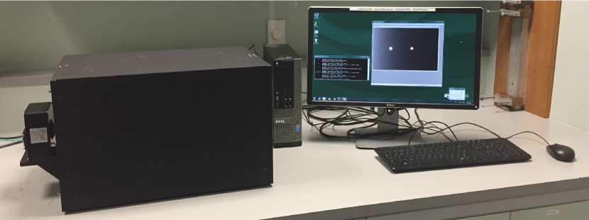
Figure 1: A picture of the experimental apparatus: the light box, star simulator (hidden), CCD camera, and acquisition computer.

In the following sections we describe in detail the experimental apparatus and the analytical tools required to extract the periodicities that are present in the detected time-series data. We also provide a few insights into the physics of pulsating WDs.

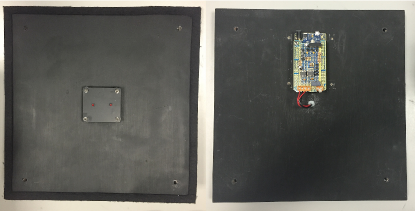
Figure 2: Close-up photos of one end plate of the light box show the LEDs and the star simulator unit that drives their intensity.

II Experimental Apparatus

The experimental apparatus (pictured in Fig. 1) consists of a light-tight box with the SBIG CCD camera and a small lens at one end imaging a pair of LEDs attached to a plate on the inside of the box at the other end. This configuration allows the CCD to be removed for general inspection, and to adjust the relative position of the lens in order to optimize the focus.

A key part of the apparatus is the ‘star simulator’ unit (pictured in Fig. 2) that drives the LEDs with simulated intensity profiles corresponding to the behaviour of chosen astronomical objects. It is attached to a panel of the box at the opposite end to the CCD and connects to the LEDs which are on the inside.

The core of the simulator electronics is an Arduinoarduino microcontroller, with a custom daughter-board (made from an off-the-shelf prototyping ‘shield’ and through-hole electronic components) that holds the LED drivers. A DC-DC converter outputs $\pm$12V to power the drivers, and an output relay is included such that one of the output channels can be redirected to an external LED, which can be viewed directly by eye outside the box. Fig. 3 gives a schematic overview of the star simulator hardware.

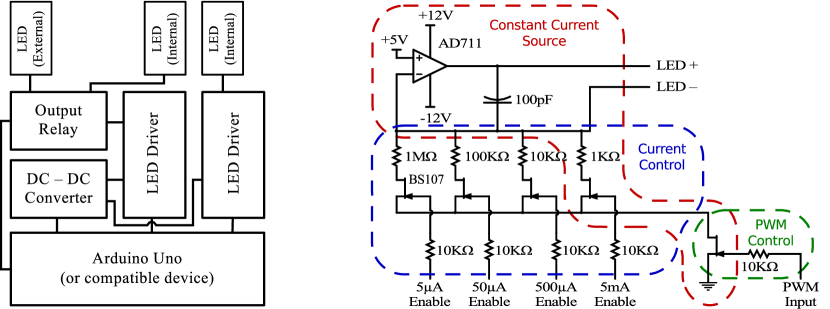
Figure 3: Block diagrams depicting the star simulator hardware. The left-hand diagram shows the functional components of the simulator. The right-hand diagram shows the LED driver circuit, which includes pulse-width modulated constant-current sources.

Each of the two LED drivers are built around an AD711 operation amplifier (op-amp) configured as a constant current source. In this configuration, the output current is determined by the resistance between the anode of the LED and ground. The output driver provides four software-selectable currents (5 $\mu$A, 50 $\mu$A, 500 $\mu$A, 5 mA) by connecting four parallel resistors (with different values) in series with individual BS107 field-effect transistors. These transistors are connected to digital output pins on the Arduino, and act as software-controlled switches that can be switched set the effective resistance to ground. All four paths run through a fifth transistor, which is connected to one of the pulse width modulation (PWM) outputs on the Arduino. This transistor is used to rapidly switch the LED on and off (using a 10-bit timer at 250 Hz) to provide 1024 fine-grained intensity levels between zero and the maximum intensity set by the current source. The combination of current and PWM control provide the large dynamic range that is required for our simulations.

The software programming (firmware) inside the Arduino is relatively straightforward. When the unit is powered on it reads the desired simulation parameters from read-only memory, and configures the current selector transistors and the PWM timers. The unit then enters a mode where it will evaluate and update the LED intensities every 16 ms and checks for new commands from the USB connection to the control PC.

We have developed four types of simulation profiles for our experiment: (a) a constant intensity; (b) a sum of multiple sinusoids (with arbitrary amplitude, frequency and phase); (c) a sum of multiple gaussians (with fixed repeating period, but arbitrary amplitude, width, and offset within a cycle); (d) a repeating linear ramp (with configurable period). These profiles provide the building blocks to define a range of simulations (such as the examples described in Section IV) and apparatus tests.

In addition to these profile types, a cloud simulation can be enabled on a per-profile basis to attenuate both output channels in a semi-random manner. A simple random number generator (based on the relative drift of two on-board oscillators) seeds control point values for a spline interpolation algorithm, which results in a smoothly varying attenuation as a factor of time. Additional per-point noise could be included to provide a more realistic simulation, but we omit this for the sake of experimental simplicity.

The profile parameters for each simulation are defined in the firmware, and uploaded to the unit via its USB connection. The active profile can be changed at any time by running a simple configuration tool on the acquisition computer.

III Data acquisition and analysis

The main steps required in the experiment are (a) acquisition of a sequence of CCD frames imaging the illuminated LEDs, (b) extraction of the LED intensities from each of the frames. (c) conversion of the LED intensities to form an appropriate time series for Fourier analysis, and (d) performing the Fourier analysis on various time series light curves and interpreting the results. We discuss each of these steps in turn.

III.1 CCD frame acquisition

After selection of one of the simulation light curve options, the first step is to acquire a sequence of $N$ CCD frames using a chosen sampling cycle time of $t_{\rm R}$ s. Each frame will have some exposure length $\Delta t$ s, which will typically be shorter than $t_{\rm R}$ s by some amount due to the CCD readout time and possibly other hardware constraints. With the SBIG CCD (ST-402ME) we use in our laboratory experiment, the minimum value for $t_{\rm R}$ is about 1 s, but the exposure times can be much shorter as the device uses a mechanical shutter (which is standard) to block the light input during the readout phase.

Clearly some thought needs to be put into deciding on the these values for a chosen simulation run such that the Nyquist criterion (a minimum of two samples for the shortest period) is met for the highest frequency in the light curve, and the run length $Nt_{\rm R}$ s is adequate to provided sufficient frequency resolution in the Fourier analysis.

In order to provide uniformity, a conventional CCD chip will measure the stored charge (formally electron-hole pairs in the Si semiconductor substrate) in each pixel serially, using a single amplifier and ADC (Analogue to Digital Converter). This conversion can take quite some time (seconds or more), especially when operated at slow speeds in order to reduce measurement noise; consequently, exposure intervals even in the many seconds domain become rather inefficient and one can end up closing the telescope to scarce photons for a significant fraction of an observing run.

The Puoko-nuipuokonui photometers employ frame transfer CCDs, which have adjacent masked pixel arrays of the same size that act as storage regions. The integrated charges in the exposure frames can be rapidly shifted to the storage frames (in milliseconds) and the frames can then be digitized and read out in parallel with the next exposure. Thus the CCD photometers can be operated without mechanical shutters, and the deadtime losses become negligible.

The laboratory simulation experiment of course doesn’t suffer from a deficit of photons so the standard CCD is perfectly adequate for the task in hand. The SBIG CCD has a fast ($\sim$ms) readout time, and so the readout dead time is not of practical concern for this experiment. Thinking in terms of LED brightness variations with periods of $\sim\,10^{2}$ s to match the real white dwarf variations, exposure times of $\sim\,10$ s or less are appropriate and provide sample rates significantly higher than the minimum Nyquist rate corresponding to the highest frequency variation in the light curves.

For their use in astronomical observing, CCDs need to be cooled below ambient temperatures in order to minimize the thermal creation of electron-hole pairs that contribute to the background. This can now be mostly achieved thermoelectrically; for example when observing, we cool our Puoko-nui South primary CCD to $-50\,$C. For the laboratory experiment, with control over the brightness of the LEDs, this can be avoided, but in the interests of alerting students to the issue it is sensible to implement cooling. Our SBIG CCD can be thermoelectrically cooled and we typically operate it at $-5$ C.

Another factor which shouldn’t remain hidden from students is the issue of dark frames. These are exposures with the shutter closed and employing the same time interval as the observation frames: they are subtracted from the latter to produce the science frames. With our SBIG CCD, the manufacturer-provided acquisition software includes options to automate this procedure. In real astronomical observing, after dark frame subtraction, the remaining background is dominated by the sky brightness, which will vary with the conditions; for the experiment in a light-tight box, this should in theory be zero. In practice, however, a finite charge is added to each pixel before digitization in order to ensure better linearity. Zero time exposures to measure these values are known as bias frames in the CCD literature. The dark subtraction also removes this bias charge. This fact should at least be mentioned in any notes in order to satisfy questions from any inquisitive students.

It is perhaps relevant to point out that when using our frame transfer CCD in shutterless mode, we need to accumulate a separate library of suitable CCD dark frames outside an observing run.

Although it is not a required step in the laboratory experiment, it would be appropriate to at least mention the part played by “flat fields” in CCD astronomical photometry. Invariably because of the telescope optics, an external uniformly bright field does not produce a uniform pixel count across the CCD. This can be accounted for by observing a physical flat field in high precision and scaling the science frame pixel counts accordingly. In practice, a flat field is obtained in astronomy by observing the bright clear sky at dusk or dawn (and removing any stellar images) or a uniformly illuminated board in the telescope dome. (And we will simply mention the debate concerning which is better).

Finally, the brightest intensity of the LEDs should be monitored, and the exposure time should be chosen such that the image intensity will not saturate. The ADCs used to digitize the pixel charges have a finite number of digital bits. In the case of our SBIG CCD, a 16 bit ADC is used yielding a maximum count of $2^{16}-1=65\,535$ ADU (analog to digital units). In practice it is best to maintain the signal of interest at a level below this maximum value.

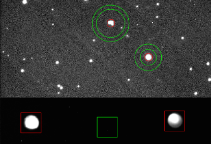
Figure 4: A composite picture comparing the two applications of the synthetic aperture technique discussed in the text in order to extract intensities from CCD frames. The upper section of the figure corresponds to a real observing frame (of the object QU Tel) and depicts the circular apertures, while the lower section is an image of two light box LEDs and illustrates the simpler square aperture method.

The number of exposures collected for the time series should ensure that a reasonable number of complete cycles of the longest period are covered and understanding the significance of this can also be part of the experiment.

III.2 Extracting LED intensities

For the real observing situation with Puoko-nui we have written code that employs circular synthetic apertures to extract stellar intensities from each exposure frame. The software package, tsreducepuokonui , uses two concentric apertures centered on each stellar image of interest to obtain the stellar intensity above the sky background, and the developing light curves are presented in real time as the observing proceeds. The top section of Fig. 4 illustrates the technique using a real observational science frame of the pulsating white dwarf QU Telxcov15 (also known as EC 20058$-$5234). It was obtained as part of an observing campaign in 2011 with the Puoko-nui South photometer attached to the Mt John one metre telescope in New Zealand. The top encircled image corresponds to the pulsating white dwarf, while the other object acts as a comparison.

For the simulation experiment the optics are much simpler and one need not be unduly concerned with the circular symmetry of telescope optics and the resulting point spread function (including the effects of astronomical “seeing” at the observing site). Instead it is both simpler and adequate to employ synthetic square apertures to determine the integrated LED flux and the background value (refer to the bottom section of Fig. 4). A close to optimum estimate of the LED intensity per frame is obtained by subtracting the summed pixels in the background aperture from the summed pixels in the LED enclosed aperture.

This approach is straightforward to implement in a computing environment such as MATLAB or Python, and if deemed appropriate the students themselves can develop their own extraction code as part of the experimental method.

It is relevant to point out that the synthetic aperture technique (square or circular) for extracting intensities is only really suitable for sparse stellar fields; with the aim of making connections where appropriate with real observing, we simply mention here the techniques of “point spread function” fitting and “difference imaging” for conducting photometry in more crowded fields. We refer the interested reader to the extensive literature for explanations of these techniques.

III.3 Creation of the time series

The information of interest in the light curves is encoded in the variations about the mean level. The actual detected intensity is rarely of interest in the world of astronomy and one is almost always required to account for the effects of flux variations created by cloud interference and changing airmass. One approach to making these corrections is to compute the normalized ratio of the variable star intensity to a nearby (constant) comparison star. This situation can be simulated if required in the experiment.

The appropriate form for the time-series data prior to performing a Fourier analysis is to compute modulation values: percentage variation in intensity units are an obvious scale to use, but millimodulation intensity (mmi) units are often used in the white dwarf pulsation literature as they are suitable for the typical $\sim 1$% intensity variations of these stars: 10 mmi corresponds to a 1% modulation in the time domain. Units consistent with these in Fourier amplitude space (see below) are millimodulation amplitude (mma) values. Furthermore, for periodicities in the $\sim 10^{2}$ s region, $10^{-3}$ Hz or mHz are suitable for frequency values. We will use these units in this paper.

III.4 Fourier analysis of the time-series data

Starting with the time series data featuring modulation intensities versus time, this step involves “simply” computing a discrete Fourier Transform (DFT) of the data. However, given the simulation data to be analyzed can include multiple frequencies (with close spacings) and has high frequency stability and coherence (that match the observed white dwarf pulsations), there are a number of features and techniques that can be exploited that will give students good insights into the use of Fourier analysis. We will simply summarize the main features here and allude to their use in the world of pulsating white dwarf asteroseismic research.

First, it is important to note that the analysis will be using a discrete version of the Fourier Transform, and to be aware of its properties and limitations. The phase information is of no interest in WD asteroseismic research, so computing the sinusoidal power (the power spectrum) will yield the amplitude of the periodicities; and, as it is best to think in terms of amplitudes rather than power (see below) we require the square root of the power spectrum, which we will call the Fourier amplitude spectrum or simply DFT henceforth.

No doubt in most circumstances the DFT will be obtained by a “black box” function (by using MATLAB routines for example), but it is important to make clear in student minds the difference between a DFT and the FFT (Fast Fourier Transform). The FFT is nothing more than an efficient way of computing a DFT — with definite limitations. For an FFT algorithm the samples must be evenly spaced, and in order to achieve maximum efficiency the number of samples needs to be a power of 2 (which is often achieved in practice by zero padding). Furthermore, the number of points in the frequency domain is dictated by the number of time domain samples; this can be a limitation when inspecting a FFT of real data, particularly with noise included.

Given the speed of modern computers we have found in practice that it is much more useful to use the most simple (but inefficient) DFT algorithm, with direct control over the number and spacing of the frequency domain estimates. This is especially so and essential when combining different data sets that have different sampling intervals and times, as sometimes occurs in multi-site observing campaigns run by groups such as the Whole Earth Telescope (WET)wet ; xcov15 .

Second, we need to introduce the concept of the DFT window and, for real life observing campaigns, generalize the concept somewhat. In the general Fourier literature the DFT standard window function is the sinc ($\sin x/x$) function (actually sinc² for power), which is the Fourier transform of a rectangular “top-hat” function that defines the finite length of the time domain sample. The DFT of the actual data is then a convolution of this sinc function and the Fourier transform of the theoretically infinite sinusoids in the data. In some applications, tapering the “top-hat” ends in order to reduce the amplitude of the wiggles in the sinc function (at the expense of broadening the central peak) is considered effective. This is called apodisation in the literature.

However, in the world of pulsating white dwarfs in particular, with the occurrence of unavoidable data gaps due to such things as cloud interference and the rising of the Sun, what is needed is a direct transformation of the signal turning on and off (often multiple times) into the Fourier domain. This is achieved by computing the DFT of a single noise free sinusoid with a suitable period calculated for each sample time for the real data. This function can be compared with various peaks in the DFT of the real data in order to see if they are consistent with only one frequency. Even if the experiment is limited to investigating the noise-free simulation light curves, it is instructive to compute the window function when examining light curves with multiple gaps and closely spaced frequencies.

Finally, in the interests of completeness and making connections with real observational data, it is relevant to discuss the impact of noise on the frequency identification process. As part of generating the light curves, observational uncertainties or noise can easily be added using for example an algorithmic (pseudo-)random number generator. The issue of identifying as real low level peaks in the DFT computed from an observational light curve is an important part of the analysis in observational astronomy.

A technique that has proved to be useful, especially in the case of low amplitude periodicities that are close to large amplitude ones, is referred to as prewhiteningxcov15 . One identifies the periods of the larger amplitude peaks in the DFT and then uses these to compute a synthetic light curve. This synthetic light curve is then subtracted from the real time-series data and another DFT calculated for the now “prewhitened” data. This new DFT should provide a clearer indication of the reality of any remaining peaks above any nearby noise peaks.

If the periodicities $T_{i}$ of the peaks being subtracted are known accurately enough, they can be fixed in a straight forward linear least squares procedure by fitting values for $A_{i}$ and $B_{i}$ in functions of the following form

$$f(t)=A_{i}\sin\left[\frac{2\pi t}{T_{i}}\right]+B_{i}\cos\left[\frac{2\pi t}{T_{i}}\right]=C_{i}\sin\left[\frac{2\pi t}{T_{i}}+\phi_{i}\right]$$

Alternatively, the $T_{i}$ values can also be optimized using nonlinear least squares techniques, which require iterative procedures. In this case, it would more convenient to also optimize the parameters $C_{i}$ and $\phi_{i}$ in the above functions.

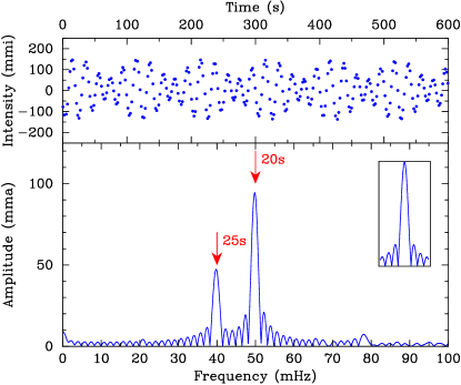
Figure 5: Modulation time series data (top panel) and the corresponding amplitude DFT (bottom panel) for a 600 s run using a sampling rate if 1 s. The LED intensity has been modulated by two frequencies with periods of 20 s and 25 s and different amplitudes, which leads to the visible beating. The sample window function is shown in the insert.

It is instructive to compare the amplitudes $C_{i}$ of the least squares derived sinusoids with those in the DFT amplitude spectrum. Of course something would be radically wrong if they were not very similar, but making the comparison reinforces the basic fact that the least squares estimates and the DFT amplitudes should be very similar even though they are derived from apparently different procedures. With this comparison in mind, it is useful to view the DFT as a set of cross correlations of the time-series data with a sequence of sinusoids with different frequencies.

When deciding whether a peak in a DFT corresponds to a real periodicity in the light curve, it is important to have a statistical model for the time domain noise and its effect on the uncertainties in the DFT. With the speed of modern computers, simulation procedures can make this task largely model-free. We are attracted to a simulation implementationxcov15 of the false alarm probability (FAP) conceptscargle for characterizing uncorrelated noise levels in DFTs. This method is intuitively straight forward and essentially free of complicated statistical theory. It is certainly preferable to simply quoting some formula for the DFT noise level.

One first prewhitens (removes) the main periodicities from the light curve, leaving residuals that characterize the time-domain noise level. The time stamps for each of the sample values are then randomly shuffled, thus destroying any remaining coherent signals in the data, but leaving the random noise level intact. A DFT of the time-shuffled data is calculated and the height of the highest peak in the region of interest is noted. This procedure is repeated N times and a record kept of each highest peak, resulting in an ensemble of highest peaks. One then asserts that there is a one in $N$ chance of the highest ensemble peak occurring through a noise conspiracy in the data. For $N=1000$ say the chance or FAP is 1 in 1000. Thus, if a peak is visible in the DFT at this level, there is 0.1% chance of it simply being noise. It is instructive to construct a histogram of the ensemble of highest peaks obtained in the simulation — some examples can be found in the referencesxcov15 .

The implementation and effectiveness (along with some explanations) of the above techniques can be found in a papers describing observational programs on pulsating white dwarfsxcov15 ; ec04207 . In particular, an implementation of a FAP simulation procedure should really make use of the much more efficient FFT algorithm given the requirement to compute a large sample of DFTs.

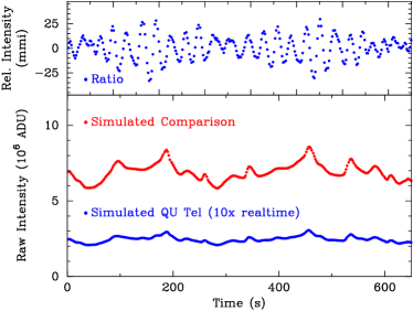
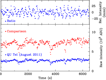
Figure 6: The low level white dwarf pulsations can be disguised or completely hidden by cloud variations. The simulated cloud effect (left panel) features a smooth intensity change, but avoids the large per-point noise that is often introduced when observing through real cloud (right panel). In both cases, the WD pulsations can be recovered by dividing the (absolute) intensity of the target star by a constant comparison star: the cloud affects both measurements equally (however note that there are second-order effects that reduce this in real observations), and this multiplicative factor cancels in the division.

IV Some Example Procedures

In this section we provide three example cases with different light curves.

The first one involves sampling a light curve that features beating between two sinusoidal signals. This provides a good starting example as it provides a relatively simple signal while the students are familiarizing themselves with the general operation of the camera and the data reduction procedures. It also illustrates the main features associated with sampling a signal with two adjacent sinusoidal signals over a finite interval. Fig. 5 depicts both the set of modulated time series samples covering an interval of 600 s and the resulting DFT. The DFT window function for this sample is also shown in the insert.

The second example employs a light curve generated using multiple frequencies corresponding to those observed in the pulsating white dwarf QU Telxcov15 (also known as EC 20058$-$5234). Cloud simulation (affecting both LED intensities) is also added to the mix and the correct light curve variations recovered by computing intensity ratios after background estimates have been subtracted (refer to Fig.6).

Fig. 7 compares a 10 h run using the QU Tel simulated light curve with a real $\sim$10 h 2004 observing run on this pulsating white dwarf carried out at Mt John Observatory in New Zealand xcov15 . Included in the figure is a comparison of the two DFTs.

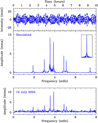
Figure 7: A 10 hour collection run (top) on a “cloudless” real-time simulation of QU Tel provides a very realistic result when compared with real observational data (bottom). The insert in the upper figure shows the DFT window for the siumulation. This simulation configuration would be suitable for a longer-form project where the students are able to set up a data collection run overnight. A shorter collection period can be used at the expense of a poorer frequency domain resolution. Alternatively, the frequency and intensity can be increased by 10$\times$ to accelerate the data collection time to only 1 hour.

The final example illustrates the principles of signal folding, and provides an impressive example of the ability to reconstruct periodic signals from sparsely sampled data when there is a high level of signal coherency. The simulation profile is based on optical observations of the pulsar (PSR B1919+21) in the Crab nebula that were acquired in 2013 using the Puoko-nui North photometerpuokonui .

A pulsar is a rotating neutron star that emits two beams of radiation such that if one of the beams intersects the Earth it is detected (primarily) in the radio frequency domain as an extremely stable periodic signal. The Crab pulsar is one of a handful that have also been detected optically. The first Crab pulsar optical detections were obtained via photometry synchronized to the known radio ephemeris crab_cocke ; crab_nather , but one can also achieve the detection using signal folding as shown in this simulation example.

Because the SBIG camera has a maximum frame rate of 1 frame per second, the 33 ms period of the simulation has been increased by a factor of 100 $\times$ to a more manageable $\sim 3.3\,s$; this yields roughly three frames sampled per pulsation cycle.

Figure 8 shows the raw time series acquired in a 10 minute collection run and the DFT of this data. The pulsation profile is non-sinusoidal (it is modelled using two gaussians), and so the main features in the frequency domain are the fundamental pulsation period and its harmonics. The shape of the pulsation profile in the time domain are encoded in the relative amplitude and phase of the harmonics in the frequency domain.

The DFT plot shows another important aspect of Fourier analysis: frequencies that are greater than the Nyquist frequency (500 mHz for these 1 s samples) are ‘aliased’ back inside the DFT range by reflection around either the Nyquist frequency (at the high end) or zero (at the low). It can be difficult to distinguish aliases from true signals, but in this case we can uniquely identify the fundamental frequency based on the known time-domain period (which can be timed manually using the external LED on the lightbox), and it is then a straightforward exercise to identify the remaining peaks by taking integer multiples of the fundamental frequency and applying the appropriate reflections.

The precise period of the pulsar signal can be identified from the DFT plot, and this period is then used to ‘fold’ the signal over itself in order to create a detailed form for a single pulsation cycle. This can be represented mathematically using the equation

$$\phi_{i}=\frac{t_{i}}{T}-\left\lfloor\frac{t_{i}}{T}\right\rfloor\,,$$

where $\left\lfloor\ \right\rfloor$ denotes the integer division operator (divide and discard the remainder). In other words, we are converting the time-based signal to a phase (which may be itself measured as a time, angle, or fractional number). This is shown in Figure 9, which compares the simulated pulsar photometry against our real observational data.

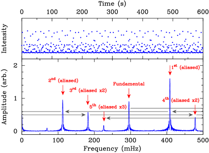
Figure 8: The time series data (upper panel) obtained as part of the pulsar example and its DFT (lower panel). This example illustrates the effect of DFT aliasing in undersampled signals and the utility of data folding at a known period (refer to text).

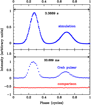
Figure 9: The simulated pulsar time series data folded at the known period (upper plot) compared with the actual Crab pulsar folded data (and a nearby comparison) obtained in 2013 using the Puoko-nui North photometer. The Crab and comparison data have been binned (see referencepuokonui ).

V Discussion

We have outlined a range of topics connected with the observation of pulsating white dwarf stars that can be explored using our simulation apparatus. Depending on the course level that the experiment might be offered in, one would want to make a selection of the topics discussed. During the early development of this experiment we used it very successfully as the basis of a one semester project in 2013 in our 400-level Honours course in physics, and in 2014 it was run as a 200-level experiment.

Ideally, a laboratory experiment using the simulator should endeavor to draw as many links as possible to the real world of astronomical observing and the physics of the target objects. The pulsating white dwarfs are certainly a suitable subject for this task.

When white dwarfs pulsate (at several well-defined surface temperature regimes) they are usually multiperiodic and exhibit very stable frequencies. This is largely a consequence of their compact very slowly evolving structure – about the mass of the Sun compressed into a sphere about the size of the Earth. They are prevented from gravitational collapse by the temperature-independent degeneracy pressure resulting from the essentially separate electron gas in the plasma being gravitationally confined at very high number densities.

The observed luminosity variations result from nonradial gravity mode pulsations — the more common and intuitively simpler radial pulsations due to pressure variations (seen in many other stellar types) have never been observed in white dwarfs. The underlying driving mechanism for stellar pulsation is the interaction of the escaping core radiation with a partially ionized chemical element (usually H or He) in a layer near the star’s surface. This mechanism was first postulated by Eddingtoneddington early last century.

For white dwarfs, the very high surface gravities clearly inhibit radial material motion and hence limit any consequent luminosity variations. In addition, the large bulk modulus (high “stiffness”) of the material leads to high sound speeds and hence to expected periodicities of seconds or less for the pressure modes. These oscillations, if they exist, are likely to be very difficult to detectsilvotti11 ; kilkenny14 .

The gravity modes, however, are the result of material density gradients in the local gravitational field and feature much longer periods: the so-called Brunt-Väisälä frequencywinget determines these periods and its calculated values are consistent with the hundreds of seconds luminosity variations seen in the pulsating white dwarfs. A simplified and instructive physical picture for the phenomenon is to envisage the oscillations of an object floating at the interface between two fluids of different density (eg water and air).

However, in white dwarfs the gravity modes involve largely nonradial material motion and a rich array of possible normal modes. It is interesting to note that the gravity mode pulsations in white dwarfs were discoveredlandolt before a theoretical model was proposed.

A final note on the asteroseismic study of white dwarfs is worth making and should be at least mentioned in any experimental notes. The detected frequencies in a pulsating white dwarf are used to infer normal modes of the star and these are used to guide and constrain theoretical models of the structure. Including some of these steps in an experiment is possible, but it would take us beyond the scope of this article.

Obviously, the apparatus could also be used to simulate other observational programs by generating appropriate synthetic light curves: eclipsing binary stars, planetary transit events, or even gravitational microlensing events involving extrasolar planets orbiting starsulensing are interesting possibilities.

From an observer’s perspective, simulating the observation of the short period binary object NY Vir (also known as PG 1336$-$018)pg1336 ; puokonui provides an interesting experience: it has a $\sim$2.5 h period, a deep primary eclipse, a smaller secondary eclipse combined with a ‘reflection effect’ and one component is also a pulsating (subdwarf B) star. A number of classic binary star light curve characteristics are therefore in evidence, but more detailed analysis would require some advanced modelling.

Also, the detection of extrasolar planets via transits is certainly of current topical interestkepler and monitoring and analyzing a simulation light curve corresponding to a relatively rapid planetary transitjha ; djsts could make a useful laboratory experiment.

However, we think that the optimum and least artificial use of the equipment is to produce and analyse light curves corresponding to pulsating white dwarfs, develop expertise in Fourier techniques and also explore at least some of the physics of these exotic yet ubiquitous astrophysical objects.

- (1) D. J. Sullivan, “The New Zealand WET three channel photometer”, Baltic Astronomy, 9, 425–431 (2000).
- (2) P. Chote, D. J. Sullivan, R. Brown, S. T. Harrold, D. E. Winget and D. W. Chandler, “Puoko-nui: a flexible high-speed photometric system”, Mon.Not.R.Astron.Soc., 440, 1490–1497 (2014).
- (3) SBIG Astronomical Instruments website: <https://www.sbig.com>
- (4) The Arduino website: <http://www.arduino.cc>
- (5) D. E. Winget and S. O. Kepler, “Pulsating White Dwarf Stars and Precision Asteroseismology”, Ann.Rev.Astron.Ap., 46, 157– (2008).
- (6) R. E. Nather, D. E. Winget, J. C. Clemens, C. J. Hansen, and B. P. Hine, “The Whole Earth Telescope: a new astronomical instrument”, Astrophys.J., 361, 309–317 (1990).
- (7) D. J. Sullivan, T. S. Metcalfe, D. O’Donoghue et al., “Whole Earth Telescope observations of the hot helium atmosphere pulsating white dwarf EC 200585234”, Mon.Not.R.Astron.Soc., 387, 137–152 (2008).
- (8) J. D. Scargle, “Studies in astronomical time series analysis II – Statistical aspects of spectral analysis of unevenly spaced data”, Astrophys.J., 263, 835–853 (1982).
- (9) P. Chote, D. J. Sullivan, M. H. Montgomery and J. L. Provencal, “Time series photometry of the helium atmosphere pulsating white dwarf EC 04207-4748”, Mon.Not.R.Astron.Soc., 431, 520–527 (2013).
- (10) W. J. Cocke, M. J. Disney and D. J. Taylor, “Discovery of Optical Signals from Pulsar NP 0532”, Nature, 221, 525–527 (1969).
- (11) R. E. Nather, B. Warner and M. Macfralane, “Optical Pulsations in the Crab Nebula Pulsar”, Nature, 221, 527–529 (1969).
- (12) A. S. Eddington, “The Internal Constitution of the Stars”, Cambridge Univ. Press (1926).
- (13) R. Silvotti, G. Fontaine, M. Pavlov, T. R. Marsh, V. S. Dhillon, S. P. Littlefair and F. Getman, “Search for p-mode oscillations in DA white dwarfs with VLT-ULTRACAM. I. Upper limits to the p-modes”, Astron. & Astrophys., 525, A64 (2011).
- (14) D. KIlkenny, B. Y. Welsh, C. Koen, A. A. S. Gubis and M. M. Kotze, “A search for p-mode pulsations in white dwarf stars using the Berkeley Visible Imaging Tube detector”, Mon.Not.R.Astron.Soc., 437, 1836–1839 (2014).
- (15) A. U. Landolt, “A New Short-period Blue Variable”, Astrophys.J., 153, 151–164 (1968).
- (16) An interesting gravitational microlensing planetary event: B. S. Gaudi, D. P. Bennett, A. Udalski et al., “Discovery of a Jupiter/Saturn analogue with gravitational microlensing”, Science, 319, 927–930 (2008).
- (17) D. Kilkenny, M. D. Reed, D. O’Donoghue et al., “A Whole Earth Telescope campaign on the pulsating subdwarf B binary system PG 1336-018 (NY Vir)”, Mon.Not.R.Astron.Soc., 345, 834–846 (2003).
- (18) Kepler space telescope website: <http://kepler.nasa.gov>
- (19) S. Jha, D. Charbonneau, P. M. Garnavich, D. J. Sullivan, T. Sullivan, T. M. Brown and J. L. Tonry, “Multicolor observations of a planetary transit of HD 209458”, Astrophys.J., 540, L45–L48 (2000).
- (20) D. J. Sullivan and T. Sullivan, “Mauna Kea high-speed photometry of transits of the extrasolar planet HD 209458b”, Baltic Astronomy, 12, 145-165 (2003).