Vibronic origin of long-lived coherence in an artificial molecular light harvester

Abstract

Natural and artificial light harvesting processes have recently gained new interest. Signatures of long lasting coherence in spectroscopic signals of biological systems have been repeatedly observed, albeit their origin is a matter of ongoing debate, as it is unclear how the loss of coherence due to interaction with the noisy environments in such systems is averted. Here we report experimental and theoretical verification of coherent exciton-vibrational (vibronic) coupling as the origin of long-lasting coherence in an artificial light harvester, a molecular J-aggregate. In this macroscopically aligned tubular system, polarization controlled 2D spectroscopy delivers an uncongested and specific optical response as an ideal foundation for an in-depth theoretical description. We derive analytical expressions that show under which general conditions vibronic coupling leads to prolonged excited-state coherence.

Introduction

The remarkably high efficiency in photosynthesis, where nine out of ten absorbed photons reach the reaction center, is a fascinating field of modern research. In such photosynthetic complexes, structure, dynamics and function are inextricably linked. A conserved building block comprises strongly absorbing pigments arranged in close proximity to one another by a surrounding protein scaffoldvan_Grondelle ; Blankenship . Typical inter-pigment distances are of order of $10\,\AA$ and photon absorption leads to the formation of delocalized excited electronic states (excitons) shared by two or more pigment molecules. Exciton creation, migration and trapping are central to the functionality of a photosynthetic apparatus. The controlled and adjustable arrangement of the pigments tunes the electronic network and the properties of its interaction with the vibrational environment that is associated with either the pigments or the protein. The detailed balance of these properties determines the efficiency of light harvesting systemsRenger2001 ; HuelgaPlenio_CP2013 .

Exciton dynamics can be efficiently probed by two-dimensional (2D) electronic spectroscopyJonas_ARPC2003 . This technique revealed oscillatory signals in the spectral response of a wide variety of photosynthetic aggregatesEngel_Nature2007 ; Dostal2014 . Initially ascribed to excitonic beatings, oscillations have been found to persist up to several hundreds of femtoseconds at room temperatureCollini_Nature2010 ; Romero_NaturePhys2014 ; Fuller_NatureChem2014 . This time scale exceeds typical dephasing rates in the condensed phase and becomes comparable to exciton transfer timesvan_Grondelle , thus posing the question of the nature and functional relevance of these coherences HuelgaPlenio_CP2013 . Unfortunately, the complex structure of 2D signals makes the unambiguous identification of the underlying mechanisms that support such long-lived coherences a challenging task and several hypotheses to explain them have been formulated Chin_NaturePhys2013 ; Plenio_JCP2013 ; ChinHP12 ; Kolli_JCP2012 ; Jonas_PNAS2012 ; Fleming_Science2007 ; Ishizaki_PCCP2010 ; Engel_Science2013 ; Christensson_JPCB2011 ; Caycedo_JCP2012 ; Christensson_JPCB2012 . The different approaches can be classified into theories including coherent interaction of excitons with intra-pigment vibrationsChin_NaturePhys2013 ; Plenio_JCP2013 ; ChinHP12 ; Kolli_JCP2012 ; Jonas_PNAS2012 and theories focusing on incoherent exciton-protein interaction such as correlated fluctuationsFleming_Science2007 ; Ishizaki_PCCP2010 ; Engel_Science2013 . It is possible that some of these mechanisms may coexist on certain time scales and that one or another may become dominant depending on the system under consideration.

In this work, we show that the relatively simple excitonic structure of a molecular J-aggregate provides an ideal test case to identify the microscopic mechanism behind long-lived oscillations in electronic 2D-signals. The investigated J-aggregate is tubular and aligns along the sample’s flow direction when in solution. Additionally, the J-aggregate exhibits excitonic bands with roughly orthogonal transition dipole moments. It is this combination of perpendicular excitonic transitions and macroscopic alignment that makes electronic 2D-spectroscopy with polarization-controlled excitation pulses an ideal tool to study coherence effects between the excitonic bands. This approach significantly reduces the complexity of retrieved 2D signals, leading to only two peaks with oscillatory components in specific regions of the 2D-maps, i.e. one on the diagonal and one as a cross-peak for non-rephasing and rephasing signal components, respectively. Employing a vibronic model, we derive analytical expressions that show how system parameters such as electronic decoherence rates and exciton-vibrational resonance determine the amplitude and lifetime of oscillatory signals. Fitting the analytical expressions to measured data, the vibronic model achieves quantitative agreement with experimental observations. Concerning potential functional relevance of the observed oscillations, we show that the long-lived oscillatory signals in our system are dominated by excited-state coherence rather than ground-state coherence.

Results

The system. J-aggregates of cyanine dyes are promising candidates for artificial antenna systemsHeijs_CP2007 ; Wurthner_ACIE2011 ; Eisele_PNAS2014 ; Yuen-Zhou_ACSNano2014 ; Qiao_ACSNano2015 . They are chemically versatile and self-assemble into various extended supramolecular structures in aqueous solutionBerlepsch . Here a system that can be considered a macroscopically aligned synthetic light harvester was studied, namely a molecular J-aggregate of C8O3-monomers whose aggregation behavior is well knownBerlepsch2002 ; Berlepsch2003 . As revealed by cryogenic transmission electron microscopyBerlepsch_JPCB2000 , the aggregate structure is best described as a double-layered nanotube with outer diameter $\sim$$\,11\,{\rm nm}$ and lamellar spacing of $\sim$$\,2.2\,{\rm nm}$ between the chromophore layers. Additionally, superhelical bundles of these tubes can also form, though the addition of polyvinyl alcohol (PVA) inhibits this process and thereby avoids single-layered tube formationEisele_PNAS2014 and maintains a stable solution over several weeksBerlepsch_JPCB2003 . A drawing of the J-aggregate under investigation, from here on referred to as C8O3, is shown in Fig.1a. The bilayer configuration of C8O3 allows the effect of different decoherence rates to be studied as the outer solvent-exposed layer shows faster decoherence than the inner protected layer.

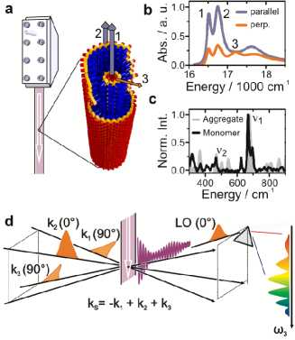
Figure 1: C8O3 and polarization controlled 2D spectroscopy. a, Wire-guided window-free jet used for sample circulation, along with a schematic of the double-layered structure of the C8O3-aggregate. The aggregates align along the flow direction (white arrow). The transition dipole directions of bands 1-3 are displayed by arrows, which are mainly polarized along the tube axis (bands 1 and 2 shown in blue) or perpendicular to the axis (band 3 shown in orange). b, Absorption spectra with light polarized parallel (blue) and perpendicular (orange) to the flow direction. c, Non-resonant Raman spectra of the C8O3-monomer (black line) and aggregate (grey area). The vibrational frequencies $\nu_{1}$ and $\nu_{2}$ are close to the exciton energy splitting between bands 1 and 3 and bands 2 and 3, respectively. d, Polarization controlled 2D spectroscopy with three excitation pulses ($k_{1}$ to $k_{3}$) and a local oscillator (LO) for heterodyne detection of the signal field, depicted as an oscillating line. Polarization orientation ($0^{\circ}$ or $90^{\circ}$) is given with respect to the longitudinal axis of aligned C8O3.

The structural properties of the aggregate are remarkable: the $11\,{\rm nm}$ outer diameter is contrasted by a length of several micrometers. Circulating solvated C8O3 with a wire-guided jet (Fig.1a) leads to a macroscopic orientation of the tubes because the longitudinal axis preferentially aligns along the flow direction. This creates anisotropy for linearly polarized light, as shown in Fig.1b. Linear dichroism measurementsBerlepsch_JPCB2003 and redox-chemistry studiesEisele2012 assign bands 1 and 2 to longitudinal transitions localized upon the inner and outer cylinders, respectively (Fig.1a). Transitions to band 3 are preferentially polarized perpendicular to the long axis of C8O3 and are shared by both layers. A detailed description of sample preparation methods and band assignments is given in the Supplementary Notes 1 and 2.

Fitting the well-defined absorption peaks of C8O3 with Lorentzian functions (see Supplementary Note 2) reveals an exciton energy difference between bands 1 and 3 of $\Delta\Omega_{31}\approx 690\,{\rm cm}^{-1}$ and $\Delta\Omega_{32}\approx 460\,{\rm cm}^{-1}$ for bands 2 and 3. Both exciton energy splittings are close to vibrational frequencies $\nu_{1}\approx 668\,{\rm cm}^{-1}$ and $\nu_{2}\approx 470\,{\rm cm}^{-1}$ observed in non-resonant Raman spectraMilota_JPCA2013 (Fig.1c). These vibrational frequencies are measured in both the monomer and aggregate Raman spectra, i.e. they are not aggregation induced Raman bands. Strongly enhanced modes at similar energies were observed in resonant Raman spectra of a related cyanine dye, and can be assigned to out-of-plane vibrationsAydin_JCP2011 . Such out-of-plane vibrations were shown to couple strongly to excitonsRich2013 . The quasi-resonance between the vibrational frequencies $\nu_{1}$ and $\nu_{2}$ and exciton energy splittings $\Delta\Omega_{31}$ and $\Delta\Omega_{32}$ provides us with an interesting scenario of possible coherent interaction between bands (excitons) and vibrationsChin_NaturePhys2013 ; ChinHP12 ; Kolli_JCP2012 ; Christensson_JPCB2012 ; Butkus2013 . Such exciton-vibrational coupling induces vibronicPlenio_JCP2013 and vibrational coherencesJonas_PNAS2012 , which can both lead to long-lived beating signals in 2D spectra. Here we emphasize that coherence in the electronic excited-state manifold is referred to as vibronic and in the ground-state manifold as vibrational. Identifying the dominant contribution is of fundamental importance because only vibronic coherence, which manifests in excited state dynamics, can enhance exciton transport and thus support light-harvesting functionWomick_JPCB2009 ; Womick_JPCB2011 ; delReyCH+13 .

Experimental results. The absorption spectrum of a light harvesting system may be heavily congested because of overlapping excitonic bands and the resulting 2D-signal would exhibit significant overlap between diagonal and cross peaks, thereby impeding further analysis. It has been suggested to employ laser pulses of different relative polarization to selectively address relevant excitation pathways to obtain a clearer 2D signalHochstrasser_CP2001 . However, the advantage of polarization controlled 2D spectroscopy has been limited by the isotropic nature of the investigated samples (an ensemble). In the experiment presented here, these problems are circumvented by the measurement of the macroscopically aligned C8O3. The transition dipole moments of bands 1 and 2 are preferentially parallel to the longitudinal axis while band 3 is orthogonal, thus allowing for optimal polarization selectivity. This combination reduces the obtained 2D maps to only two relevant peaks with negligible overlap and an up to 30 times stronger signal intensity as compared to the isotropic caseRead_PNAS2007 .

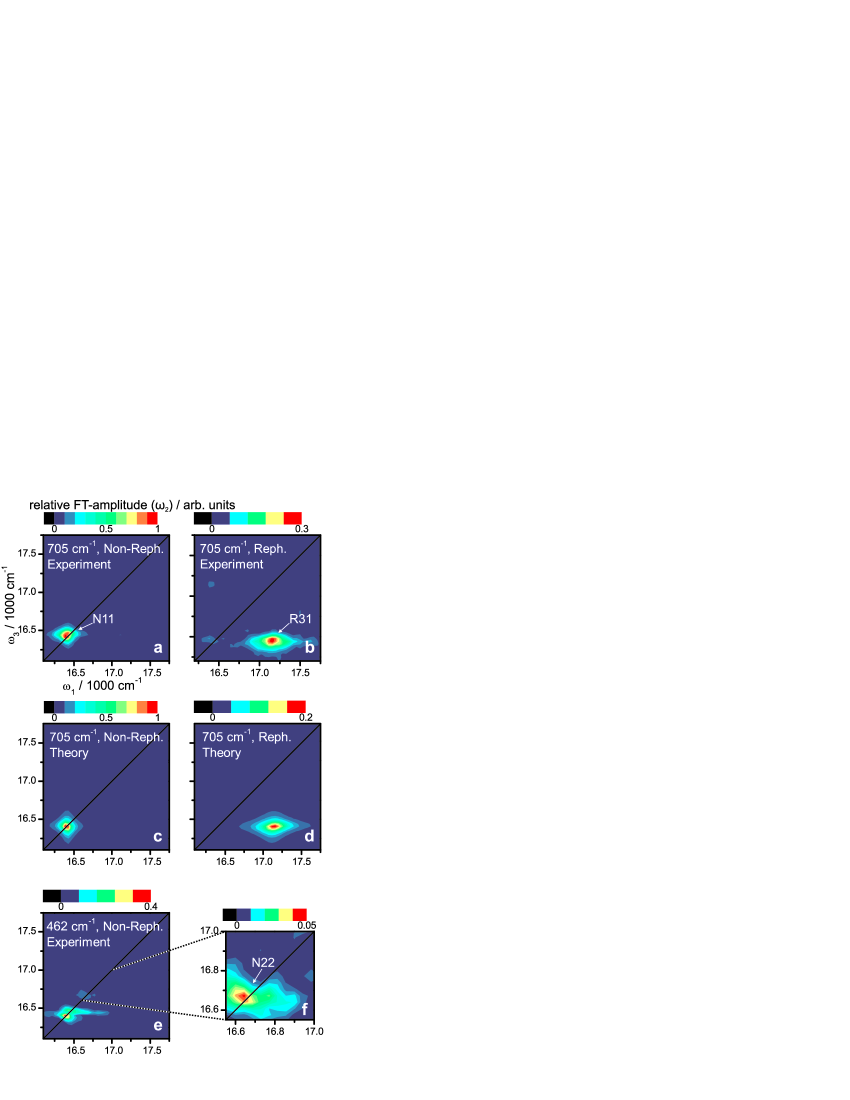
Figure 2: Experimental and theoretical 2D spectra. a, b, The Fourier-transform amplitude maps of non-rephasing and rephasing spectra at $\omega_{2}=705\pm 20\,{\rm cm}^{-1}$, which reveal the presence of a non-rephasing diagonal peak N11 and a rephasing cross-peak R31. These peaks stem from the coherent interaction of bands 1 and 3 with the quasi-resonant vibrational mode with frequency $\nu_{1}\approx 668\,{\rm cm}^{-1}$. The amplitude of N11 is about three times larger than R31. The lineshape of N11 is symmetric along both $\omega_{1}$- and $\omega_{3}$-axes, while that of R31 is elongated along $\omega_{1}$-axis. c, d, The simulated spectra at $\omega_{2}=705\,{\rm cm}^{-1}$ with N11 and R31. e, The FT amplitude map at $\omega_{2}=462\pm 20\,{\rm cm}^{-1}$ reveals coherent interaction of bands 2 and 3 with the quasi-resonant vibrational mode with frequency $\nu_{2}\approx 470\,{\rm cm}^{-1}$. However, as depicted in f, the associated non-rephasing peak N22 at $\omega_{1,3}\approx 16670\thinspace{\rm cm^{-1}}$ is weak and only amounts to 5% of N11 at $\omega_{2}=705\pm 20\,{\rm cm}^{-1}$ (see a). The diagonal peak at $\omega_{1,3}\approx 16400\thinspace{\rm cm^{-1}}$ in e stems from N11, with a peak centered at $\omega_{2}=705\pm 20\,{\rm cm}^{-1}$, but broad enough to appear at $\omega_{2}=462\pm 20\thinspace{\rm cm}^{-1}$. All measurements were carried out at room temperature.

The ideal pulse sequence to isolate beating signals between states with orthogonal transition dipole moments, i.e. bands 1 and 3 in the present case, is depicted in Fig.1d, where the phase-matched direction for measuring rephasing spectra is displayed: non-rephasing spectra can be measured along the same phase-matched signal direction by changing the order of the first two pulses (see Methods). After subtraction of the non-oscillatory background, we performed a Fourier transformation along waiting time $t_{2}$ for all points on the two-dimensional $(\omega_{1},\omega_{3})$-map. The resulting $\omega_{2}$-plots allow the lineshape of beating signal with frequency $\omega_{2}$ to be visualized as a function of position in $(\omega_{1},\omega_{3})$-space. The slice at the exciton energy splitting between bands 1 and 3 ($\omega_{2}=705\pm 20\,{\rm cm}^{-1}$ with the experimental resolution of $\pm 20\,{\rm cm}^{-1}$) reveals a non-rephasing diagonal peak N11 and a rephasing cross-peak R31 as shown in Figs.2a and b, respectively. N11 is centered at $(\omega_{1},\omega_{3})=(\Omega_{1},\Omega_{1})$ with exciton energy $\Omega_{1}\approx 16405\,{\rm cm}^{-1}$ of band 1 and a symmetric linewidth $2\Gamma_{g1}\approx 130\,{\rm cm}^{-1}$ along both $\omega_{1}$- and $\omega_{3}$-axes (Fig.2a). The center of R31 is located at $(\omega_{1},\omega_{3})=(\Omega_{3},\Omega_{1})$ with exciton energy $\Omega_{3}\approx 17125\,{\rm cm}^{-1}$ of band 3 and asymmetric linewidths $2\Gamma_{g3}\approx 300\,{\rm cm}^{-1}$ and $2\Gamma_{g1}\approx 130\,{\rm cm}^{-1}$ along $\omega_{1}$- and $\omega_{3}$-axes, respectively (Fig.2b). In peak amplitude, R31 is approximately $30\,\%$ of N11. Turning to the $\omega_{2}$-slice corresponding to the energy splitting between bands 2 and 3, ($\omega_{2}=462\pm 20\,{\rm cm}^{-1}$), Figs.2e and f reveal a diagonal non-rephasing peak N22, which is centered at $(\omega_{1},\omega_{3})=(\Omega_{2},\Omega_{2})$ with the exciton energy $\Omega_{2}\approx 16672\,{\rm cm}^{-1}$ of band 2 and a symmetric linewidth $2\Gamma_{g2}\approx 225\,{\rm cm}^{-1}$ along $\omega_{1}$- and $\omega_{3}$-axes. The amplitude of N22 is only $5\,\%$ of N11.

Theoretical model. In order to describe the long-lived oscillations in N11 and R31, a vibronic model is employed that describes the coupling of bands 1 and 3 to a quasi-resonant vibrational mode with frequency $\nu_{1}$. Consider a system with electronic ground state $\left|{g_{k}}\right\rangle$ and excited states for bands 1 and 3, denoted by $\left|{1_{k}}\right\rangle$ and $\left|{3_{k}}\right\rangle$, respectively, where $k=0$ and 1 denote the vibrational ground and excited state, respectively (Fig.3a). The vibronic coupling between the quasi-resonant states $\left|{3_{0}}\right\rangle$ and $\left|{1_{1}}\right\rangle$ leads to unnormalized vibronic eigenstates $\mathinner{\langle\tilde{3}_{0}|}=\left\langle{3_{0}}\right|+\epsilon\left\langle{1_{1}}\right|$ and $\mathinner{\langle\tilde{1}_{1}|}=\left\langle{1_{1}}\right|-\epsilon\left\langle{3_{0}}\right|$. Here, $\epsilon$ represents the degree of vibronic mixing defined by

$$\epsilon=i\nu_{1}\sqrt{S_{1}}(i\Delta\nu_{1}-\Gamma_{13})^{-1},$$

where $\Delta\nu_{1}=(\Omega_{3}-\Omega_{1})-\nu_{1}$ denotes the detuning between $\left|{3_{0}}\right\rangle$ and $\left|{1_{1}}\right\rangle$, i.e. between the exciton energy splitting and vibrational frequency, and $S_{1}$ denotes the Huang-Rhys factor of the vibrational mode, which in turn quantifies the strength of the vibronic coupling (see Supplementary Note 2 for details of the derivation). The electronic decoherence rate $\Gamma_{gk}$ describes the exponential decay rate of the coherence between electronic ground state and band $k$, while $\Gamma_{13}$ represents the overall exponential decay rate of the inter-exciton coherence between bands 1 and 3. In our model, we do not consider inhomogeneous broadening, which is justified by the observation that the experimentally measured absorption spectrum is well matched to a sum of Lorentzian functions with the linewidths $2\Gamma_{gk}$ (see Supplementary Note 2). This is valid when homogeneous broadening dominates the linewidths and the Huang-Rhys factors are sufficiently small, as is the case here. In addition, the lineshape of N11 (Fig.2a) is not elongated along the diagonal $\omega_{1}=\omega_{3}$, implying our 2D signal is dominated by homogeneous broadening. The same conclusion is reached from analyzing 2D correlation spectraMilota_JPCA2013 .

In nonlinear spectroscopy, the molecular response to laser excitation is described by response functionsMukamel . According to the vibronic model described above, the response function for the oscillatory signals in N11 reads

$${\cal R}_{N11}=\mu_{1}^{2}\mu_{3}^{2}\Gamma_{g1}^{-2}(e^{[i(\Delta\Omega_{31}+\delta\omega)-\Gamma_{13}]t_{2}}+e^{[i(\nu_{1}-\delta\omega)-\gamma_{v}]t_{2}}\epsilon^{2}),$$

with $\mu_{1}$ and $\mu_{3}$ denoting the transition dipole moment of bands 1 and 3, respectively. The prefactor $\Gamma_{g1}^{-2}$ stems from the lineshape of N11, $\gamma_{v}$ denotes the dissipation rate of the vibrations and $\delta\omega$ stands for the frequency shift of the vibronic eigenstates $\mathinner{\langle\tilde{3}_{0}|}$ and $\mathinner{\langle\tilde{1}_{1}|}$ relative to the uncoupled states $\left\langle{3_{0}}\right|$ and $\left\langle{1_{1}}\right|$ due to the vibronic coupling (see Fig.3a and Supplementary Note 2 for further details). The coupling was found to be sufficiently strong to induce non-negligible vibronic mixing $|\epsilon|^{2}\approx 0.03$, which leads to a long-lived beating signal in N11 up to $t_{2}\approx 800\,{\rm fs}$, as shown in Fig.3b. These results imply that the initial excitonic part of $\left|{1_{0}}\right\rangle\mathinner{\langle\tilde{3}_{0}|}$ decays rapidly with 1/e decay time of $\Gamma_{13}^{-1}\approx 66\,{\rm fs}$, while the vibronic coherence $\left|{1_{0}}\right\rangle\mathinner{\langle\tilde{1}_{1}|}$ explains a long-lived oscillatory signal in N11: here $\left|{1_{0}}\right\rangle\mathinner{\langle\tilde{3}_{0}|}$ ($\left|{1_{0}}\right\rangle\mathinner{\langle\tilde{1}_{1}|})$ represent coherence between two vibronic states $\left|{1_{0}}\right\rangle$ and $\mathinner{\langle\tilde{3}_{0}|}$ ($\left|{1_{0}}\right\rangle$ and $\mathinner{\langle\tilde{1}_{1}|}$), respectively.

The response function for the oscillatory contributions to R31 is given by

$${\cal R}_{R31}=\mu_{1}^{2}\mu_{3}^{2}\Gamma_{g3}^{-1}\Gamma_{g1}^{-1}(e^{[i(\Delta\Omega_{31}+\delta\omega)-\Gamma_{13}]t_{2}}+e^{[i(\nu_{1}-\delta\omega)-\gamma_{v}]t_{2}}\epsilon^{2}(\eta_{e}-\eta_{g})),$$

where $\Gamma_{g3}^{-1}\Gamma_{g1}^{-1}$ derives from the asymmetric lineshape of R31 (see Figs.2b and d). Here $\eta_{e}$ and $\eta_{g}$ represent the contribution of excited-state vibronic coherence $\left|{1_{0}}\right\rangle\mathinner{\langle\tilde{1}_{1}|}$ and ground-state vibrational coherence $\left|{g_{0}}\right\rangle\left\langle{g_{1}}\right|$, respectively, to the long-lived beating signal in R31 (see Supplementary Note 2). The vibrational coherence in the electronic ground-state manifold does not play a role in exciton transfer dynamics, but nonetheless modulates the 2D spectra. A fit of model parameters to experimental results (Fig.3c) shows that $|\eta_{e}|\approx 2.5\,|\eta_{g}|$. This means the long-lived beating signal in R31 is dominated by the excited-state coherence $\left|{1_{0}}\right\rangle\mathinner{\langle\tilde{1}_{1}|}$. The short-lived beating signal in R31 is induced by $\left|{1_{0}}\right\rangle\mathinner{\langle\tilde{3}_{0}|}$, as is the case for N11. We note that the signal at N11, with approximately three times the amplitude of R31, is exclusively determined by excited-state contributions. Details of this vibronic model and the corresponding Feynman diagrams for the spectral components N11 and R31 are discussed in the Supplementary Note 2.

These results demonstrate how an excitonic system within a noisy environment can exhibit long-lasting coherent features: the observed long-lived oscillations are the result of coherent interaction of excitonic bands with an underdamped, quasi-resonant vibration. This vibronic mechanism requires the vibrational dissipation rate $\gamma_{v}$ to be much slower than the electronic decoherence rate $\Gamma_{13}$, which is the case for C8O3, where $\gamma_{v}\lesssim(1{\rm\thinspace ps)^{-1}}$ and $\Gamma_{13}\approx(66\,{\rm fs)}^{-1}$. The difference in electronic and vibrational decoherence rates can be rationalized from the fact that excitons and vibrations are related to the motion of electrons and nuclei, respectively. The lower mass of electrons as compared to nuclei makes excitons more mobile and therefore more sensitive to environmental fluctuations, such as local electric fields, than vibrations. We note that the vibronic mixing leading to long-lived beating signals in 2D-ES is described by a vibronic coupling that induces coherent energy exchange between excitons and quasi-resonant vibrations (see Supplementary Note 2 for further details):

$$H_{e-v}=\nu_{1}\sqrt{S_{1}}(\left|{3_{0}}\right\rangle\left\langle{1_{1}}\right|+\left|{1_{1}}\right\rangle\left\langle{3_{0}}\right|).$$

This implies that the vibronic coupling not only induces long-lasting electronic excited-state coherences, but also can mediate population transfer between excitonic bands. In a combination with thermal relaxation of exciton populations, the vibronic coupling may further enhance exciton population transfer and as a result could, in principle, have functional relevance in exciton transportWomick_JPCB2011 ; Kolli_JCP2012 ; Perlik_JCP2015 ; Killoran_arXiv2015 ; Schroter_PR2015 .

Interestingly, the different decoherence rates $\Gamma_{g3}\approx 2\Gamma_{g1}$ of bands 1 and 3 lead to different amplitudes of the short-lived beating signals in N11 and R31 (Figs.3b and c), which are determined by the prefactors $\Gamma_{g1}^{-2}$ and $\Gamma_{g3}^{-1}\Gamma_{g1}^{-1}$, respectively. The lower decoherence rate of band 1 can be explained by band 1 being localized on the inner layer, while band 3 is delocalized over both the inner and outer layersDidraga_JPCB2004 . As shown by the response functions for N11 and R31, the overall strength of the beating signals is proportional to the inverse of the electronic decoherence rates. It is therefore expected that the beating signal amplitude would diminish with an increase of the decoherence rate. This is the case for N22, where the physical situation in terms of exciton-vibrational resonance ($\Delta\Omega_{32}\approx\nu_{2}\approx 470\,{\rm cm}^{-1}$) is equivalent to N11 ($\Delta\Omega_{31}\approx\nu_{1}\approx 668\,{\rm cm}^{-1}$). The crucial difference is that band 2 has a higher decoherence rate than band 1, as band 2 is localized on the outer layer exposed to solventDidraga_JPCB2004 . This explains the broader linewidth of band 2 in absorption and 2D spectra. Using an estimated value of $\Gamma_{g2}\approx(47\,{\rm fs)}^{-1}$, the presented theory predicts the strength of N22 to be $5\,\%$ of N11 (see Supplementary Note 2), which is in line with the experimental observations (Fig.2f). These results indicate that the experimentally observed long-lived beating signals, induced by vibronic mixing, require adequately low electronic decoherence rates, highlighting that resonance between exciton energy splitting and vibrational frequency alone is not sufficientMiller_NatureChem2014 .

The presented vibronic model achieves quantitative agreement with the experimental observations. Crucially, the constraints imposed by the observed asymmetric decoherence rates $\Gamma_{g3}\approx 2\Gamma_{g1}$ and fast relaxation of exciton population in C8O3 on sub-picosecond timescalesMilota_JPCA2013 rule out incoherent models, where long-lived oscillations are sustained by Markovian correlated fluctuations (see Supplementary Note 3 for a detailed analysis). This further supports our conclusion that the observed experimental data provide evidence for vibronic mixing being the mechanism at play in our system.

We note that our results do not imply that correlated fluctuations can be universally ruled out, as this mechanism could be in place in certain pigment-protein complexes. The notion of correlated fluctuations has been developed for photosynthetic complexes where pigments are embedded in a protein scaffold. The protein has been considered as the potential source of correlated fluctuations in natural light harvestersFleming_Science2007 ; Ishizaki_PCCP2010 . For C8O3, a structural frame such as a protein scaffold is absent and therefore correlated fluctuations are unlikely to induce long-lived oscillatory 2D-signals, which is in line with our observations.

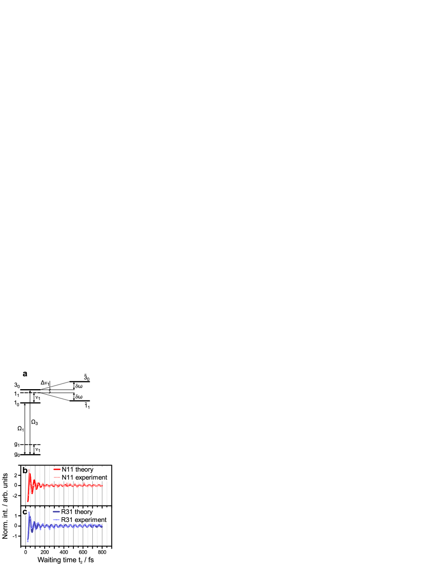
Figure 3: Vibronic model. a, We consider a vibronic model for bands 1 and 3 coupled to a vibrational mode with frequency $\nu_{1}\approx 668\,{\rm cm}^{-1}$ (see Supplementary Note 2). The vibronic states $\left|{k_{0}}\right\rangle$ and $\left|{k_{1}}\right\rangle$ denote the vibrational ground and first excited state of an electronic state $\left|{k}\right\rangle$, respectively, with the single index states $\left|{g}\right\rangle$, $\left|{1}\right\rangle$ and $\left|{3}\right\rangle$ denoting the electronic ground state and bands 1 and 3, respectively. The exciton energy splitting $\Delta\Omega_{31}=\Omega_{3}-\Omega_{1}$ between bands 1 and 3 is quasi-resonant with the vibrational frequency $\nu_{1}$, where the detuning is denoted by $\Delta\nu_{1}=\Delta\Omega_{31}-\nu_{1}$. The exciton-vibrational coupling between uncoupled states $\left|{3_{0}}\right\rangle$ and $\left|{1_{1}}\right\rangle$ leads to vibronic eigenstates $\mathinner{|\tilde{3}_{0}\rangle}$ and $\mathinner{|\tilde{1}_{1}\rangle}$, each of which is a superposition of $\left|{3_{0}}\right\rangle$ and $\left|{1_{1}}\right\rangle$, leading to an energy-level shifting by $\delta\omega$. b, The time trace of N11 where the experimental results are shown as light red circles, and the theoretical simulation is shown as a full red line. c, The time trace of R31 where the experimental results are shown as light blue circles, and the simulated data are depicted as a full blue line. The root-mean-square deviation (RMSD) between the experimental results and theoretical simulation in b and c is 0.92 and 0.59, respectively.

Discussion

We have verified, theoretically and experimentally, that coherent vibronic coupling in the electronic excited-state manifold is responsible for the long-lived beating signals observed in 2D spectra of an artificial light harvester. The relatively simple electronic and vibrational structure of the investigated molecular aggregate along with its macroscopic alignment allowed us to rule out the presence of correlated fluctuations. The specific geometry of our system allowed us to gain further insights by illustrating the conditions under which intra-pigment vibrations can prolong electronic coherent effects. The moderately low decoherence rate of band 1, localized on the inner layer and protected from solvent, is the basis for exciton-vibrational coupling as the source of long-lived beating signals. The outer band 2, even though resonantly coupled to a vibration, exhibits a higher decoherence rate and therefore fails to produce observable oscillations. We conclude that the mere resonance between excitons and vibrations does not suffice to explain long-lived beating signals. An adequately low electronic decoherence rate, determined by the interaction between system and bath, is an equally important prerequisite.

The influence of vibronic coupling on energy transport in molecular aggregates has been extensively studied in the past, as recently reviewedSchroter_PR2015 . The vibronic coupling has recently gained new interest (see ref.Chenu_ARPC2015 for a recent tutorial overview), as it was suggested as a feasible mechanism to explain long-lived oscillations in the 2D spectra of several natural light harvesting complexes and a photosynthetic reaction centerRomero_NaturePhys2014 ; Fuller_NatureChem2014 . The requirement of exciton-vibrational resonance is readily satisfied in such systems, given their numerous excitonic bands and rich vibrational structures. Incoherent models based upon correlated fluctuations were not ruled out though. Our work provides a quantum mechanical foundation for enhanced energy transfer based on vibronic coupling. As recently demonstrated, this mechanism is not limited to natural light harvesting, vibronic coupling is also of key importance in photovoltaic devicesFalke2014 .

Methods

Polarization controlled 2D electronic spectroscopy. In 2D electronic spectroscopy, three ultrashort laser pulses generate an optical response of a molecular ensemble, which is spectrally resolved along both absorption ($\omega_{1}$) and detection ($\omega_{3}$) frequencies within the laser pulse spectrum. The absorption frequency $\omega_{1}$ is obtained by precise scanning of the time delay between the first two pulses and subsequent Fourier transformation ($t_{1}\rightarrow\omega_{1}$). In detection, the signal is spectrally dispersed, leading directly to the detection frequency $\omega_{3}$. Varying time delay $t_{2}$ between pulses 2 and 3 provides information about evolution of the system on a femtosecond timescaleBrixner_JCP2004 ; Augulis_OE2011 ; Augulis_JOSAB2013 . In order to retrieve the purely absorptive part, the signal induced by pulses 1-3 is detected in a heterodyned fashion by interfering it with a phase-stable local oscillator pulse (LO). Polarization control is achieved by the combination of $\lambda/4$ wave plates and wire grid polarizers for each of the laser beams to select the desired polarization with high accuracy. Polarization-resolved 2D experiments change the relative contributions of distinct pathways depending on the polarization of the laser pulses, orientation of the transition dipole moments and isotropy of the sampleHochstrasser_CP2001 . Rephasing spectra were acquired with a polarization sequence of $(90^{\circ},0^{\circ},90^{\circ},0^{\circ})$ for pulses (1, 2, 3, LO), in contrast to non-rephasing spectra, where the time ordering of the first two pulses is reversed, leading to a polarization sequence of $(0^{\circ},90^{\circ},90^{\circ},0^{\circ})$. The polarization scheme used for rephasing spectra (Fig.1d) shows $0^{\circ}$ was defined to be parallel to the sample flow direction, depicted as a white arrow in Fig.1a. For a macroscopically aligned sample, this particular polarization sequence selects pathways stemming from interband coherences and vibronic mixingPlenio_JCP2013 ; Jonas_PNAS2012 , discussed throughout the paper, while pathways with all-parallel transition dipole moments such as ground state bleach, stimulated emission, excited state absorption and also vibrational wave packet excitation are suppressed. For the details regarding the experimental methods, see Supplementary Note 1. To subtract the non-oscillatory signals from 2D spectra, we employed a decay associated spectra analysisMilota_JPCA2013 , where the population decays were fitted by a sum of three 2D-spectra with individual decay constants. The $\omega_{2}$-maps in Fig. 2 were obtained using Fourier transformation ($t_{2}\rightarrow\omega_{2}$) with zero-padding up to $2^{7}$ data points. All measurements were carried out at room temperature.

References

Acknowledgements

The authors would like to thank Valentyn I. Prokhorenko for help in 2D-DAS analysis. C.N.L. and J.H. acknowledge funding by the Austrian Science Fund (FWF): START project Y 631-N27 and by COST Action CM1202 - PERSPECT-H2O. J.L., F.C.-S., S.F.H. and M.B.P. acknowledge funding by the EU STREP PAPETS and QUCHIP, the ERC Synergy Grant BioQ, the Deutsche Forschungsgemeinschaft (DFG) within the SFB/TRR21 and an Alexander von Humboldt Professorship. J.P. acknowledges funding by the Spanish Ministerio de Economía y Competitividad under Project No. FIS2012-30625. D.P. and D.Z. acknowledge funding by the Swedish Research Council and Knut and Alice Wallenberg Foundation.

Author contributions

D.P., D.Z. and J.H. designed and conducted experiments. H.v.B. was responsible for sample preparation, structural characterization and Raman measurements. J.L., F.C.-S., C.N.L., D.P., J.P., and J.H. analyzed the data. J.L., F.C.-S., S.F.H., J.H. and M.B.P. developed theory. All authors discussed the results and wrote the manuscript.

Competing financial interests

The authors declare no competing financial interests.

Correspondences and requests for materials should be addressed to J.H. (juergen.hauer@tuwien.ac.at).

Supplementary Information

I Experiment

I.1 Sample preparation

The monomer, tetrachlorobenzimidacarbocyanine chromophore with two attached hydrophobic octyl groups (FEW-Chemicals, Wolfen, Germany) was dissolved in $10^{-2}$ M NaOH solution to achieve a concentration of $10^{-4}$ M. The solution was then stirred in the dark for several hours. Subsequently, polyvinyl alcohol (PVA) of molecular weight $\sim$130000 was added in 1:10 w/w ratio (monomer:PVA) to slow down the formation of aggregate bundles during the storage of dye solutions. Moreover, the adsorbed PVA chains Dekany_2001_SI obviously prevent the reassembly of double-layered into single-layered tubes upon bundling. This effect was observed recently for another derivative Eisele_PNAS2014_SI (C8S3) of the present dye. The individual tubular aggregates degrade in that case into single-layered tubes, which is accompanied by a dramatic change of absorption spectra. Similar effects were not observed for C8O3 when PVA is present. In particular, the aggregate solutions prepared in the described way were stable for approximately ten days when stirred continuously. Without stirring the spectral signature of the double-layered tubes retained even after 12 weeks of storage Berlepsch_JPCB2003_SI . For 2D experiments, we additionally diluted the sample with $10{}^{-2}$ M NaOH to obtain optical density below 0.3 at 598 nm at a path length of 200 $\mu{\rm m}$.

A total sample volume of approximately 10 ml was circulated through the U-shaped wire-guided jet Tauber_RSI2003_SI by a peristaltic pump (Masterflex C/L) with a flow speed optimized for film stability. Solvent evaporated from the recollecting container was refilled every 4 hours during the course of 13 hour measurement.

I.2 Data acquisition

Passively stabilized 2D spectroscopy was described in detail elsewhere Brixner_JCP2004_SI . Briefly, a home-built non-collinear optical parametric amplifier (NOPA) seeded by $180\,{\rm fs}$ pulses at $1030\,{\rm nm}$ from PHAROS (Light Conversion Ltd) was tuned to generate $\sim$$16\,{\rm fs}$ pulses ($80\,{\rm nm}$ full width at half maximum) centered at $580\,{\rm nm}$. The NOPA output was split into four pulses and arranged in the so-called boxcar geometry. Waiting time $t_{2}$ was controlled by a mechanical translation stage (PI), whereas coherence time $t_{1}$ was scanned by inserting a pair of fused silica wedges into the first two pulses. All four pulses were focused and overlapped in the sample. The first three generated a third order nonlinear optical response which is emitted in the photon echo phase-matched direction. This signal was heterodyned with an attenuated fourth pulse, called local oscillator (LO). The resulting interference pattern was spectrally resolved and detected by a CCD camera (PIXIS, Princeton Instruments). Most of the scatter was eliminated by the double-frequency lock-in modulation of the first two pulses Augulis_OE2011_SI . The polarization of each pulse was controlled by the combination of $\lambda/4$ wave plates and wire grid polarizers (contrast ratio $>800$). The accuracy of the polarization angle was estimated to be $\pm 1^{\circ}$, where the unwanted signals were typically suppressed by a factor of $\sim$80 for the selected polarization sequence.

To prevent degradation of the sample, the power and repetition rate of the laser were set to $200\,{\rm pJ/pulse}$ and $40\,{\rm kHz}$, respectively. Spectral resolution of $\sim$$35\,{\rm cm}^{-1}$ for the detection frequency $\omega_{3}$ was determined by the grating, the number of CCD pixels and Fourier filtering of the signal during the standard analysis procedure. Coherence time was scanned from $-300\,{\rm fs}$ to $384\,{\rm fs}$ in $1.5\,{\rm fs}$ steps, providing $\sim$$43\,{\rm cm}^{-1}$ spectral resolution of absorption frequency $\omega_{1}$. Waiting time steps of $12\,{\rm fs}$ were sufficient to resolve oscillatory features up to $1350\,{\rm cm}^{-1}$ with $\sim$$35\,{\rm cm}^{-1}$ resolution along $\omega_{2}$.

I.3 Polarization-controlled 2D-ES

The strength of 2D signals is determined by the scalar products of molecular transition dipole moments and pulse polarizations. To take advantage of i) the preferential orientation of the J-aggregate (from here on referred to as C8O3) along the flow direction of the jet and ii) mutually perpendicular transition dipole moments of bands 1(2) and 3 of C8O3, we designed a polarization scheme selective for interband coherences. This is similar to the case of an isotropic sample discussed both theoretically Hochstrasser_CP2001_SI and experimentally SchlauCohen_NC2012_SI ; Westenhoff_JACS2012_SI . In the presented experiments, the polarization scheme for rephasing signals reads $(90,0,90,0)$ for beams 1-4, respectively. The first and third pulses, polarized orthogonal (90) to the jet’s flow direction, interact with bands 1-3. The second pulse, polarized parallel (0) to the jet’s flow direction, interacts preferentially with bands 1 and 2, due to the negligible transition dipole moment of band 3 along this direction. The polarization scheme for non-rephasing spectra reads $(0,90,90,0)$, as the ordering of the first two pulses is reversed. These polarization schemes restrict oscillatory signals induced by interband coherences to the lower cross peak in rephasing spectra (R31) and the lower diagonal peak in non-rephasing spectra (N11), as shown in Figures 2 and 3 of the main text. Non-oscillatory 2D signals were subtracted prior to Fourier transformation $t_{2}\rightarrow\omega_{2}$.

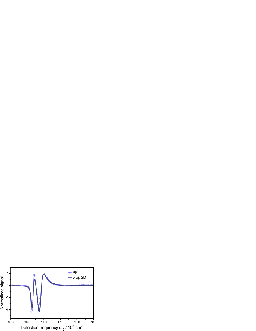
Figure 4: Pump-probe and projected 2D signal. Projection of phased polarization-controlled 2D spectra (blue) to all-parallel pump-probe (light blue) at $\mathrm{t_{2}=180\,fs}$.

The polarization-controlled 2D spectra were phased to pump-probe data where pump and probe pulses were polarized in parallel. This procedure is not rigorously correct because in polarization-controlled 2D-ES the first two pulses have different polarization directions while in pump-probe the first two interactions derive from the same pump pulse which naturally means parallel interactions. In other words, the projection slice theorem is strictly speaking not valid for the experiments presented here Jonas_ARPC2003_SI . Despite this discrepancy, one can still satisfactorily phase polarization-controlled 2D spectra to all-parallel pump-probe as shown in Supplementary Figure 4. One explanation of this is leakage of the much stronger all-parallel signals through the crossed polarizers, meaning that the all-parallel signal still dominates the non-oscillatory part of the (90,0,90,0) 2D-signal. In this work, we decided to phase polarization-controlled 2D data to parallel pump-probe data. We note that the imperfection in phasing parameters only affects the lineshapes of the real and imaginary part of $\omega{}_{2}$ maps, but preserves their amplitude-maps in both lineshape and magnitude. Hence, the difficulties in phasing polarization-controlled 2D spectra discussed above do not affect the conclusions drawn in the main part of the main text, which were based on $\omega{}_{2}$ amplitude-maps. To this end, we found that arbitrary and large changes of the phasing parameters do not alter $\omega{}_{2}$ amplitude-maps shown in Figure 2 of the main text (results not presented). It is noted that sophisticated phasing techniques based on heterodyned transient grating instead of pump-probe offer a correct method to phase crossed-polarization 2D signals Milota_OE2013_SI .

II Theory

II.1 A vibronic model for bands 1 and 3 of C8O3

In the following the vibronic model used to describe bands 1 and 3 of C8O3 and simulate 2D spectra is described. We consider coherent interaction of bands 1 and 3 with the intramolecular vibrational modes of frequency $\hbar\nu_{1}\approx 668\,{\rm cm}^{-1}$, which is quasi-resonant with the exciton energy splitting between bands 1 and 3. The environmental noise induced by background phonons (a phonon bath) is modeled by a Markovian quantum master equation.

II.1.1 Hamiltonian

The electronic Hamiltonian of C8O3 that consists of a network of cyanine dye molecules is described by

$$H_{e} =\sum_{\alpha}\hbar E_{\alpha}\left|{e_{\alpha}}\right\rangle\left\langle{e_{\alpha}}\right|+\sum_{\alpha\neq\beta}\hbar J_{\alpha\beta}\left|{e_{\alpha}}\right\rangle\mathinner{\langle{e_{\beta}}|}$$ (1)

$$=\sum_{k}\hbar\Omega_{k}\left|{k}\right\rangle\left\langle{k}\right|,$$ (2)

where $\left|{e_{\alpha}}\right\rangle$ represents the excited state of site $\alpha$ (or molecule $\alpha$), $E_{\alpha}$ denotes the site energy including electronic and reorganization energies, and $J_{\alpha\beta}$ the electronic coupling between sites $\alpha$ and $\beta$. The diagonalization of the electronic Hamiltonian $H_{e}$ gives rise to the exciton states $\left|{k}\right\rangle=\sum_{\alpha}\left|{e_{\alpha}}\right\rangle\mathinner{\langle e_{\alpha}|k\rangle}$ associated with the exciton energies $\Omega_{k}$, where bands 1 and 3 are denoted by $\left|{1}\right\rangle$ and $\left|{3}\right\rangle$, respectively: $\mathinner{\langle e_{\alpha}|k\rangle}\in R$ for $E_{\alpha},J_{\alpha\beta}\in R$.

The vibrational modes with frequency $\hbar\nu_{1}\approx 668\,{\rm cm}^{-1}$ are described by a set of harmonic oscillators

$$H_{v}=\sum_{\alpha}\hbar\nu_{1}a^{\dagger}_{\alpha}a_{\alpha},$$ (3)

where $a^{\dagger}_{\alpha}$ and $a_{\alpha}$ represent the creation and annihilation operators, respectively, of the intramolecular vibrational mode of site $\alpha$. The interaction between vibrations and the electronic excitation of molecules is modeled by

$$H_{e-v}=\sum_{\alpha}\hbar\nu_{1}\sqrt{s_{1}}\left|{e_{\alpha}}\right\rangle\left\langle{e_{\alpha}}\right|(a^{\dagger}_{\alpha}+a_{\alpha}),$$ (4)

where $s_{1}$ denotes the Huang-Rhys factor of the vibrational modes. In the exciton basis $\{\left|{k}\right\rangle\}$, the interaction Hamiltonian $H_{e-v}$ is represented by

$$H_{e-v}=\hbar\nu_{1}\sqrt{s_{1}}\sum_{k,l}\left|{k}\right\rangle\left\langle{l}\right|\sum_{\alpha}\mathinner{\langle k|e_{\alpha}\rangle\langle e_{\alpha}|l\rangle}(a^{\dagger}_{\alpha}+a_{\alpha}),$$ (5)

where the diagonal terms ($k=l$) lead to adiabatic surfaces in the electronic excited states, called vibrons, while the non-diagonal terms ($k\neq l$) induce coherent transition between different excitons mediated by exciton-vibrational couplings.

In this work, we are interested in the coherent interaction of bands 1 and 3 with the quasi-resonant vibrational modes of frequency $\nu_{1}$, which is described by the following cross term $\tilde{H}_{e-v}$ in Eq. (5)

$$\tilde{H}_{e-v}=\hbar\nu_{1}\sqrt{S_{1}}(\left|{1}\right\rangle\left\langle{3}\right|+\left|{3}\right\rangle\left\langle{1}\right|)(\tilde{a}^{\dagger}_{1}+\tilde{a}_{1}),$$ (6)

where $\tilde{a}_{1}=N\sum_{\alpha}\mathinner{\langle 1|e_{\alpha}\rangle\langle e_{\alpha}|3\rangle}a_{\alpha}$ describes an effective vibrational mode with frequency $\nu_{1}$. Here $N$ is introduced to normalize the effective vibrational mode, such that $[\tilde{a}_{1},\tilde{a}^{\dagger}_{1}]=1$, leading to an effective Huang-Rhys factor $S_{1}=s_{1}/N^{2}$. This implies that for a given Huang-Rhys factor $s_{1}$, the effective Huang-Rhys factor $S_{1}$ is increased as the spatial overlap $\mathinner{\langle 1|e_{\alpha}\rangle\langle e_{\alpha}|3\rangle}$ between excitonic wavefunctions of bands 1 and 3 increases, leading to smaller $N$ and larger $S_{1}=s_{1}/N^{2}$. The effective Hamiltonian of bands 1 and 3 coupled to the effective vibrational mode is then described by $\tilde{H}=\tilde{H}_{e}+\tilde{H}_{v}+\tilde{H}_{e-v}$, where $\tilde{H}_{e}=\hbar\Omega_{1}\left|{1}\right\rangle\left\langle{1}\right|+\hbar\Omega_{3}\left|{3}\right\rangle\left\langle{3}\right|$ and $\tilde{H}_{v}=\hbar\nu_{1}\tilde{a}^{\dagger}_{1}\tilde{a}_{1}$. We note that the vibrational energy $\hbar\nu_{1}\approx 668\,{\rm cm}^{-1}$ is higher than the thermal energy $k_{B}T\approx 208\,{\rm cm}^{-1}$ at room temperature $T=300\,K$, implying that the thermal state of the vibrational mode is well approximated by its ground state. In addition, when exciton-vibrational couplings are sufficiently small, the light-induced vibrational excitation of overtones is negligible due to the small Franck-Condon factors. This is the case for C8O3, where N11 and R31 in 2D spectra can be well described within a subspace spanned by $\{\left|{g_{0}}\right\rangle,\left|{g_{1}}\right\rangle,\left|{1_{0}}\right\rangle,\left|{1_{1}}\right\rangle,\left|{3_{0}}\right\rangle\}$. Here, $\left|{k_{0}}\right\rangle$ and $\left|{k_{1}}\right\rangle$ denote the vibrational ground and first excited states of an electronic state $\left|{k}\right\rangle$, respectively, i.e. $(\tilde{H}_{e}+\tilde{H}_{v})\left|{k_{l}}\right\rangle=\hbar(\Omega_{k}+l\nu_{1})\left|{k_{l}}\right\rangle$, where $\left|{g}\right\rangle$ represents the electronic ground state with $\Omega_{g}=0$. In this scenario, $\{\left|{1_{0}}\right\rangle,\left|{3_{0}}\right\rangle\}$ can be directly excited by light from the ground state $\left|{g_{0}}\right\rangle$, while $\{\left|{g_{1}}\right\rangle,\left|{1_{1}}\right\rangle\}$ has an extremely low transition probability due to small Franck-Condon factors. Nonetheless, $\{\left|{g_{1}}\right\rangle,\left|{1_{1}}\right\rangle\}$ can be populated through exciton-vibrational coupling $\nu_{1}\sqrt{S_{1}}$, leading to transition from $\left|{3_{0}}\right\rangle$ to $\left|{1_{1}}\right\rangle$, and subsequently to $\left|{g_{1}}\right\rangle$ via emission. The coherent transition between $\left|{3_{0}}\right\rangle$ and $\left|{1_{1}}\right\rangle$ requires resonance between vibrational frequency $\nu_{1}$ and exciton energy splitting $\Delta\Omega_{31}=\Omega_{3}-\Omega_{1}$ between bands 1 and 3, i.e. $\Delta\Omega_{31}\approx\nu_{1}$.

II.1.2 Decoherence

In addition to the coherent interaction of bands 1 and 3 with the effective vibrational mode $\tilde{a}_{1}$, we consider electronic decoherence induced by background phonons. We characterize the decoherence by two dynamical processes, i) the incoherent population transfer between excitons, called exciton relaxation, and ii) the pure dephasing noise that destroys electronic coherence without exciton population transfer. In addition, we consider iii) relaxation of the effective vibrational mode.

We assume that each cyanine dye molecule is coupled to an independent phonon bath. The Hamiltonian of the background phonons is given by $H_{\rm ph}=\sum_{\xi}\hbar\upsilon_{\xi}b^{\dagger}_{\xi}b_{\xi}$ with the interaction Hamiltonian $H_{e-{\rm ph}}=\sum_{\alpha,\xi}\hbar g_{\alpha\xi}\mathinner{|e_{\alpha}\rangle\langle e_{\alpha}|}(b_{\xi}^{\dagger}+b_{\xi})$ between molecules and phonons, where $b_{\xi}^{\dagger}$ and $b_{\xi}$ denote the creation and annihilation operators, respectively, of a background phonon mode $\xi$. Here $g_{\alpha\xi}$ represents the exciton-phonon coupling between site $\alpha$ and phonon mode $\xi$, which satisfies $g_{\alpha\xi}g_{\beta\xi}=0$ for all $\beta\neq\alpha$, implying that when site $\alpha$ is coupled to the phonon mode $\xi$ with $g_{\alpha\xi}\neq 0$, all the other sites $\beta$ are decoupled from the mode with $g_{\beta\xi}=0$. For the sake of simplicity, we assume that there is no degeneracy in the exciton energies $\Omega_{k}$, which leads to a relatively simple form of a Markovian quantum master equation. This condition is satisfied even if the exciton energies are close to degeneracy unless they are strictly degenerate, which is satisfied for bands 1 and 3 of our interest. The influence of the background phonons on the vibronic system consisting of bands 1 and 3 with the effective vibrational mode is then described by a Markovian quantum master equationBreuer_SI

$$\frac{d}{dt}\rho(t)=-\frac{i}{\hbar}[\tilde{H},\rho(t)]+{\cal D}_{r}[\rho(t)]+{\cal D}_{d}[\rho(t)]+{\cal D}_{v}[\rho(t)],$$ (7)

where $\rho(t)$ denotes the reduced vibronic state, while ${\cal D}_{r}[\rho(t)]$, ${\cal D}_{d}[\rho(t)]$ and ${\cal D}_{v}[\rho(t)]$ describe exciton relaxation, pure dephasing noise and relaxation of the effective vibrational mode, respectively.

i. Exciton relaxation
Here ${\cal D}_{r}[\rho(t)]$ describes exciton relaxation

$${\cal D}_{r}[\rho(t)] =\sum_{\omega\neq 0}\sum_{\alpha}\gamma_{\alpha\alpha}(\omega)\left(A_{\alpha}(\omega)\rho(t)A_{\alpha}^{\dagger}(\omega)-\frac{1}{2}\{A_{\alpha}^{\dagger}(\omega)A_{\alpha}(\omega),\rho(t)\}\right),$$ (8)

with $\Delta\Omega_{kl}=\Omega_{k}-\Omega_{l}$ denoting the exciton energy splitting between $\left|{k}\right\rangle$ and $\left|{l}\right\rangle$, $A_{\alpha}(\omega)=\sum_{k,l}\delta(\omega,\Delta\Omega_{kl})\left\langle l|e_{\alpha}\right\rangle\left\langle e_{\alpha}|k\right\rangle\left|{l}\right\rangle\left\langle{k}\right|$ for $\omega\neq 0$, leading to incoherent transition from $\left|{k}\right\rangle$ to $\left|{l}\right\rangle$, where $\delta(i,j)$ denotes the Kronecker delta defined by $\delta(i,j)=1$ if $i=j$ and $\delta(i,j)=0$ otherwise. In Eq. (8), $\gamma_{\alpha\alpha}(\omega)$ is defined by

$$\gamma_{\alpha\alpha}(\omega)=2\pi{\cal J}_{\alpha}(\omega)(n(\omega)+1),$$ (9)

with $n(\omega)=(\exp(\hbar\omega/k_{B}T)-1)^{-1}$ representing the Bose-Einstein distribution function at temperature $T$, ${\cal J}_{\alpha}(\omega)$ is the spectral density of site $\alpha$ defined by ${\cal J}_{\alpha}(\omega)=\sum_{\xi}g_{\alpha\xi}^{2}\delta(\omega-\upsilon_{\xi})$ if $\omega\geq 0$ and ${\cal J}_{\alpha}(\omega)=-{\cal J}_{\alpha}(-\omega)$ otherwise. Here $\delta(x)$ represents the Dirac delta function defined by $\delta(x)\rightarrow\infty$ if $x=0$ and $\delta(x)=0$ otherwise with $\int_{-\infty}^{\infty}dx\delta(x)=1$.

ii. Pure dephasing noise
${\cal D}_{d}[\rho(t)]$ in Eq. (7) describes the pure dephasing noise

$${\cal D}_{d}[\rho(t)]=\sum_{\alpha}\gamma_{\alpha\alpha}(0)\left(A_{\alpha}(0)\rho(t)A_{\alpha}^{\dagger}(0)-\frac{1}{2}\{A_{\alpha}^{\dagger}(0)A_{\alpha}(0),\rho(t)\}\right),$$ (10)

where $A_{\alpha}(0)=\sum_{k}\left|\left\langle k|e_{\alpha}\right\rangle\right|^{2}\left|{k}\right\rangle\left\langle{k}\right|$ destroys electronic coherence without changing exciton populations defined by $\{{\rm Tr}[\left\langle{k}\right|\rho(t)\left|{k}\right\rangle]\}$.

By substituting electronic coherences $\left|{g}\right\rangle\left\langle{1}\right|$, $\left|{g}\right\rangle\left\langle{3}\right|$ and $\left|{1}\right\rangle\left\langle{3}\right|$ to the dissipators ${\cal D}_{r}[\rho(t)]$ and ${\cal D}_{d}[\rho(t)]$ in Eqs. (8) and (10), one can obtain the following electronic decoherence rates $\Gamma_{g1}$, $\Gamma_{g3}$ and $\Gamma_{13}$ of the coherences $\left|{g}\right\rangle\left\langle{1}\right|$, $\left|{g}\right\rangle\left\langle{3}\right|$ and $\left|{1}\right\rangle\left\langle{3}\right|$

$$\Gamma_{g1} =\frac{1}{2}\sum_{l\neq 1}\gamma_{1\rightarrow l}+\gamma_{g1},$$ (11)

$$\Gamma_{g3} =\frac{1}{2}\sum_{l\neq 3}\gamma_{3\rightarrow l}+\gamma_{g3},$$ (12)

$$\Gamma_{13} =\frac{1}{2}\sum_{l\neq 1}\gamma_{1\rightarrow l}+\frac{1}{2}\sum_{l\neq 3}\gamma_{3\rightarrow l}+\gamma_{13},$$ (13)

where $\gamma_{k\rightarrow l}$ denotes the incoherent population transfer rate from band $k$ to $l$

$$\gamma_{k\rightarrow l}=\sum_{\alpha}\gamma_{\alpha\alpha}(\Delta\Omega_{kl})\mathinner{|\langle l|e_{\alpha}\rangle\langle e_{\alpha}|k\rangle|}^{2}\geq 0,$$ (14)

while $\gamma_{g1}$ and $\gamma_{g3}$ represent the pure dephasing rates of the coherences $\left|{g}\right\rangle\left\langle{1}\right|$ and $\left|{g}\right\rangle\left\langle{3}\right|$, respectively,

$$\gamma_{g1} =\frac{1}{2}\sum_{\alpha}\left|\left\langle 1|e_{\alpha}\right\rangle\right|^{2}\gamma_{\alpha\alpha}(0)\mathinner{|\langle 1|e_{\alpha}\rangle|}^{2},$$ (15)

$$\gamma_{g3} =\frac{1}{2}\sum_{\alpha}\left|\left\langle 3|e_{\alpha}\right\rangle\right|^{2}\gamma_{\alpha\alpha}(0)\mathinner{|\langle 3|e_{\alpha}\rangle|}^{2},$$ (16)

and $\gamma_{13}$ represents the pure dephasing rate of the inter-exciton coherence $\left|{1}\right\rangle\left\langle{3}\right|$ between bands 1 and 3

$$\gamma_{13}=\frac{1}{2}\sum_{\alpha}\left(\left|\left\langle 1|e_{\alpha}\right\rangle\right|^{2}-\left|\left\langle 3|e_{\alpha}\right\rangle\right|^{2}\right)\gamma_{\alpha\alpha}(0)\left(\mathinner{|\langle 1|e_{\alpha}\rangle|}^{2}-\mathinner{|\langle 3|e_{\alpha}\rangle|}^{2}\right).$$ (17)

These results imply that the inter-exciton dephasing rate $\gamma_{13}$ should be lower than the sum of the other dephasing rates $\gamma_{g1}$ and $\gamma_{g3}$ when there is a spatial overlap between excitonic wavefunctions of bands 1 and 3

$$\gamma_{13}=\gamma_{g1}+\gamma_{g3}-\sum_{\alpha}\left|\left\langle 1|e_{\alpha}\right\rangle\right|^{2}\gamma_{\alpha\alpha}(0)\mathinner{|\langle 3|e_{\alpha}\rangle|}^{2}\leq\gamma_{g1}+\gamma_{g3},$$ (18)

with $\gamma_{\alpha\alpha}(0)\geq 0$ for all $\alpha$, the equality $\gamma_{13}=\gamma_{g1}+\gamma_{g3}$ holds if and only if there is no spatial overlap between excitonic wavefunctions, i.e. $\left|\left\langle 1|e_{\alpha}\right\rangle\right|^{2}\left|\left\langle 3|e_{\alpha}\right\rangle\right|^{2}=0$ for all $\alpha$, or the spectral densities ${\cal J}_{\alpha}(\omega)$ of the molecules shared by bands 1 and 3 do not induce pure dephasing noise by $\gamma_{\alpha\alpha}(0)=0$ for all sites $\alpha$ satisfying $\left|\left\langle 1|e_{\alpha}\right\rangle\right|^{2}\left|\left\langle 3|e_{\alpha}\right\rangle\right|^{2}\neq 0$. This implies that even if each molecule is coupled to an independent phonon bath, the spatial overlap between excitonic wavefunctions can reduce the inter-exciton dephasing rate $\gamma_{13}$. Here the independent phonon baths of the molecules shared by excitons effectively form a common phonon bath coupled to both excitons, leading to a partial dephasing-free subspace. For instance, if bands 1 and 3 have perfect spatial overlap, i.e. $\left|\left\langle 1|e_{\alpha}\right\rangle\right|^{2}=\left|\left\langle 3|e_{\alpha}\right\rangle\right|^{2}$ for all $\alpha$, while the orthogonality between them is satisfied by the phases of $\left\langle 1|e_{\alpha}\right\rangle\left\langle e_{\alpha}|3\right\rangle$, i.e. $\mathinner{\langle 1|3\rangle}=\sum_{\alpha}\mathinner{\langle 1|e_{\alpha}\rangle\langle e_{\alpha}|3\rangle}=0$, the inter-exciton dephasing rate $\gamma_{13}$ will become zero, as each $A_{\alpha}(0)=\sum_{k}\left|\left\langle k|e_{\alpha}\right\rangle\right|^{2}\left|{k}\right\rangle\left\langle{k}\right|=\left|\left\langle 1|e_{\alpha}\right\rangle\right|^{2}(\left|{1}\right\rangle\left\langle{1}\right|+\left|{3}\right\rangle\left\langle{3}\right|)+\sum_{k\neq 1,3}\left|\left\langle k|e_{\alpha}\right\rangle\right|^{2}\left|{k}\right\rangle\left\langle{k}\right|$ forms a dephasing-free subspace $\left|{1}\right\rangle\left\langle{1}\right|+\left|{3}\right\rangle\left\langle{3}\right|$ of bands 1 and 3. Since band 1 is localized on the inner layer of C8O3, while band 3 is delocalized on both the inner and outer layersDidraga_JPCB2004_SI , there is a partial spatial overlap between excitonic wavefunctions, leading to $\gamma_{13}<\gamma_{g1}+\gamma_{g3}$. The spatial overlap is also required for a non-zero value of the effective Huang-Rhys factor $S_{1}$, which is responsible for the long-lived beating signals observed in the experiment, as will be discussed later.

In addition, the inter-exciton dephasing rate $\gamma_{13}$ has a non-zero lower bound when the dephasing rates $\gamma_{g1}$ and $\gamma_{g3}$ are different in magnitude. The dephasing rates in Eqs. (15)-(17) can be expressed as $\gamma_{g1}=\mathinner{|\vec{v}_{1}|}^{2}$, $\gamma_{g3}=\mathinner{|\vec{v}_{3}|}^{2}$ and $\gamma_{13}=\mathinner{|\vec{v}_{1}-\vec{v}_{3}|}^{2}$ with the real vectors $\vec{v}_{k}$ defined by $\vec{v}_{k}=2^{-1/2}\hat{\gamma}^{1/2}\vec{w}_{k}$, where $\vec{w}_{k}$ is a real vector with elements $\left|\left\langle k|e_{\alpha}\right\rangle\right|^{2}\geq 0$ representing the delocalization of an exciton state $\left|{k}\right\rangle$ in the site basis $\{\left|{e_{\alpha}}\right\rangle\}$, while $\hat{\gamma}$ is a diagonalized matrix with elements $\gamma_{\alpha\alpha}(0)\geq 0$, leading to a positive matrix $\hat{\gamma}^{1/2}$ defined by $\hat{\gamma}=\hat{\gamma}^{1/2}\hat{\gamma}^{1/2}$. From the triangle inequality, $\mathinner{|\vec{v}_{1}-\vec{v}_{3}|}+\mathinner{|\vec{v}_{3}|}\geq\mathinner{|\vec{v}_{1}|}$ and $\mathinner{|\vec{v}_{1}-\vec{v}_{3}|}+\mathinner{|\vec{v}_{1}|}\geq\mathinner{|\vec{v}_{3}|}$, the inter-exciton dephasing rate $\gamma_{13}$ is bounded from below by $(\sqrt{\gamma_{g1}}-\sqrt{\gamma_{g3}}~{})^{2}$, leading to $(\sqrt{\gamma_{g1}}-\sqrt{\gamma_{g3}}~{})^{2}\leq\gamma_{13}<\gamma_{g1}+\gamma_{g3}$. Therefore, the electronic decoherence rate $\Gamma_{13}$ of the inter-exciton coherence $\left|{1}\right\rangle\left\langle{3}\right|$ is constrained by

$$\frac{1}{2}\sum_{l\neq 1}\gamma_{1\rightarrow l}+\frac{1}{2}\sum_{l\neq 3}\gamma_{3\rightarrow l}+\left[\left(\Gamma_{g1}-\frac{1}{2}\sum_{l\neq 1}\gamma_{1\rightarrow l}\right)^{1/2}-\left(\Gamma_{g3}-\frac{1}{2}\sum_{l\neq 3}\gamma_{3\rightarrow l}\right)^{1/2}~{}\right]^{2}\leq\Gamma_{13}<\Gamma_{g1}+\Gamma_{g3},$$ (19)

with $\gamma_{gk}=\Gamma_{gk}-\frac{1}{2}\sum_{l\neq k}\gamma_{k\rightarrow l}$ from Eqs. (11) and (12). Here the population transfer rates ($\gamma_{1\rightarrow l}$ and $\gamma_{3\rightarrow l}$) and electronic decoherence rates ($\Gamma_{g1}$ and $\Gamma_{g3}$) can be estimated using experimentally measured 2D spectra, which will be discussed later.

iii. Relaxation of quasi-resonant vibrations
Finally, ${\cal D}_{v}[\rho(t)]$ in Eq. (7) describes the relaxation of the effective vibrational mode

$${\cal D}_{v}[\rho(t)]=\gamma_{v}(n(\nu_{1})+1)\left(2\tilde{a}_{1}\rho(t)\tilde{a}_{1}^{\dagger}-\{\tilde{a}_{1}^{\dagger}\tilde{a}_{1},\rho(t)\}\right)+\gamma_{v}n(\nu_{1})\left(2\tilde{a}_{1}^{\dagger}\rho(t)\tilde{a}_{1}-\{\tilde{a}_{1}\tilde{a}_{1}^{\dagger},\rho(t)\}\right).$$ (20)

Since $n(\nu_{1})\approx 0.04$ at room temperature $T=300\,K$ due to the high vibrational energy $\hbar\nu_{1}\gg k_{B}T$, Eq. (20) can be reduced to

$${\cal D}_{v}[\rho(t)]\approx\gamma_{v}\left(2\tilde{a}_{1}\rho(t)\tilde{a}_{1}^{\dagger}-\{\tilde{a}_{1}^{\dagger}\tilde{a}_{1},\rho(t)\}\right),$$ (21)

which describes the dissipation of the vibrational mode with the rate of $\gamma_{v}$.

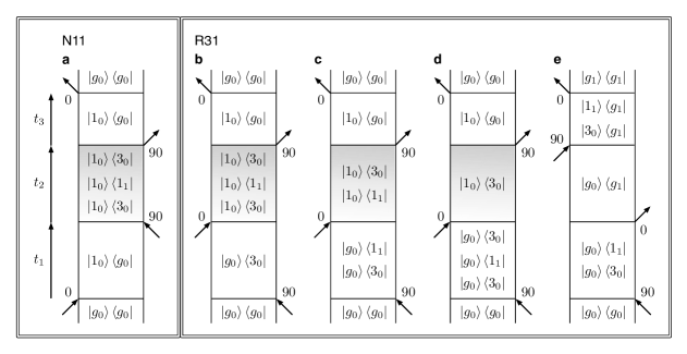
Figure 5: Feynman diagrams contributing to the beating signals in N11 and R31 represented in uncoupled state basis. a, The stimulated emission diagram contributing to the beating signals in N11. Here time runs upwards and the electronic transitions induced by light are denoted by arrows: 0 and 90 denote the polarization of light, parallel and normal to the longitudinal axis of C8O3, respectively (cf. Figure 1 in the main text). The time interval between pulses is called coherence time $t_{1}$, waiting time $t_{2}$, and rephasing time $t_{3}$ for the first and second, the second and third, and the third excitation pulse and the emerging signal, respectively. The Fourier transform along $t_{1}$ and $t_{3}$ leads to the absorption and detection frequencies denoted by $\omega_{1}$ and $\omega_{3}$, respectively. b-e, The stimulated emission and ground state bleaching diagrams contributing to the beating signals in R31. In a-d, grey shaded waiting time periods during $t_{2}$ highlight vibronic coherences in the electronic excited states. In e, on the other hand, the vibronic system is in the electronic ground state during $t_{2}$.

II.1.3 The response function for N11

Here we derive the response function for the beating signals in N11, which is a diagonal peak in non-rephasing spectra centered at $(\omega_{1},\omega_{3})\approx(\Omega_{1},\Omega_{1})$.

In Fig. 5a, the Feynman diagram contributing to the beating signals in N11 after the employed $(0,90,90,0)$ excitation is displayed. As the thermal state of the effective vibrational mode at room temperature is well approximated by its ground state ($\hbar\nu_{1}\gg k_{B}T$), the initial state of the vibronic system is given by $\left|{g_{0}}\right\rangle\left\langle{g_{0}}\right|$. After excitation to $\left|{1_{0}}\right\rangle\left\langle{g_{0}}\right|$ by the first pulse, the dynamics of $\left|{1_{0}}\right\rangle\left\langle{g_{0}}\right|$ during coherence time $t_{1}$ is governed by a time evolution super-operator ${\cal U}(t_{1})$ determined by the quantum master equation in Eq. (7)

$${\cal U}(t_{1})\left|{1_{0}}\right\rangle\left\langle{g_{0}}\right|=e^{(-i\Omega_{1}-\Gamma_{g1})t_{1}}\left|{1_{0}}\right\rangle\left\langle{g_{0}}\right|,$$ (22)

for which the Fourier transform is given by

$$\int_{0}^{\infty}dt_{1}e^{i\omega_{1}t_{1}}{\cal U}(t_{1})\left|{1_{0}}\right\rangle\left\langle{g_{0}}\right|=-\frac{1}{i(\omega_{1}-\Omega_{1})-\Gamma_{g1}}\left|{1_{0}}\right\rangle\left\langle{g_{0}}\right|,$$ (23)

where the prefactor $-(i(\omega_{1}-\Omega_{1})-\Gamma_{g1})^{-1}$ determines the lineshape of N11 along the $\omega_{1}$-axis, which is centered at $\omega_{1}=\Omega_{1}$ with a linewidth of $2\Gamma_{g1}$. By the second pulse, $\left|{1_{0}}\right\rangle\left\langle{g_{0}}\right|$ becomes $\left|{1_{0}}\right\rangle\left\langle{3_{0}}\right|$, which evolves during waiting time $t_{2}$ into a mixture of $\left|{1_{0}}\right\rangle\left\langle{3_{0}}\right|$ and $\left|{1_{0}}\right\rangle\left\langle{1_{1}}\right|$, mediated by exciton-vibrational coupling, scaling with $\nu_{1}\sqrt{S_{1}}$. The time evolution of $\left|{1_{0}}\right\rangle\left\langle{3_{0}}\right|$ is formally expressed as

$${\cal U}(t_{2})\left|{1_{0}}\right\rangle\left\langle{3_{0}}\right|=\left|{1_{0}}\right\rangle\left\langle{3_{0}}\right|e^{Kt_{2}}=f(t_{2})\left|{1_{0}}\right\rangle\left\langle{3_{0}}\right|+g(t_{2})\left|{1_{0}}\right\rangle\left\langle{1_{1}}\right|,$$ (24)

where $K$ is a non-Hermitian operator describing both the Hamiltonian dynamics and decoherence

$$K =(i\Delta\Omega_{31}-\Gamma_{13})\left|{3_{0}}\right\rangle\left\langle{3_{0}}\right|+(i\nu_{1}-\gamma_{v})\left|{1_{1}}\right\rangle\left\langle{1_{1}}\right|+i\nu_{1}\sqrt{S_{1}}(\left|{3_{0}}\right\rangle\left\langle{1_{1}}\right|+\left|{1_{1}}\right\rangle\left\langle{3_{0}}\right|).$$ (25)

Here we evaluate $f(t_{2})$ in Eq. (24), which describes the case that $\left|{1_{0}}\right\rangle\left\langle{3_{0}}\right|$ becomes $\left|{1_{0}}\right\rangle\left\langle{g_{0}}\right|$ by the third pulse, as shown in Fig. 5a. By diagonalizing the non-Hermitian operator $K$, one can show that $f(t_{2})$ is given by

$$f(t_{2})=\sum_{k=1}^{2}\frac{1}{2}\left(1+(-1)^{k}\frac{x-y}{\sqrt{(x-y)^{2}+4z^{2}}}\right)\exp\left[\frac{1}{2}\left(x+y+(-1)^{k}\sqrt{(x-y)^{2}+4z^{2}}\right)t_{2}\right],$$ (26)

where $x=i\Delta\Omega_{31}-\Gamma_{13}$, $y=i\nu_{1}-\gamma_{v}$ and $z=i\nu_{1}\sqrt{S_{1}}$. Finally, $\left|{1_{0}}\right\rangle\left\langle{g_{0}}\right|$ evolves during rephasing time $t_{3}$

$${\cal U}(t_{3})\left|{1_{0}}\right\rangle\left\langle{g_{0}}\right|=e^{(-i\Omega_{1}-\Gamma_{g1})t_{3}}\left|{1_{0}}\right\rangle\left\langle{g_{0}}\right|,$$ (27)

for which the Fourier transform leads to the lineshape $-(i(\omega_{3}-\Omega_{1})-\Gamma_{g1})^{-1}$ of N11 along the $\omega_{3}$-axis. Therefore, the response function for N11 is given by

$$R_{1g}(\omega_{1},t_{2},\omega_{3})=\mu_{1p}^{2}\mu_{3n}^{2}\frac{1}{i(\omega_{1}-\Omega_{1})-\Gamma_{g1}}\frac{1}{i(\omega_{3}-\Omega_{1})-\Gamma_{g1}}f(t_{2}),$$ (28)

where $\mu_{1p}$ denotes the transition dipole moment of band 1 for light polarized parallel to the longitudinal axis of C8O3, while $\mu_{3n}$ represents the transition dipole moment of band 3 for light polarized normal to the axis. This is due to the $(0,90,90,0)$ polarization scheme employed for measuring non-rephasing spectra in the experiment, as schematically shown in Fig. 5a. It is notable that all the Feynman diagrams in Figs. 5a-e can be induced by $(90,90,90,90)$ excitation where all the pulses are polarized normal to the longitudinal axis: band 1 can be excited or de-excited by both 0 and 90 polarizations, although with higher efficiency for light polarized at 0. For $(90,90,90,90)$ excitation, the overall dipole strength $\mu_{1p}^{2}\mu_{3n}^{2}$ in Eq. (28) is decreased to $\mu_{1n}^{2}\mu_{3n}^{2}$ with $\mu_{1p}^{2}>\mu_{1n}^{2}$, as band 1 is mainly polarized along the longitudinal axis of C8O3, as shown in the linear dichroism spectrum in Figure 1 of the main text. This implies that the $(0,90,90,0)$ polarization scheme for non-rephasing spectra enhances the signal-to-noise ratio when compared to the $(90,90,90,90)$ excitation. Similarly, the signal-to-noise ratio of rephasing spectra is enhanced by $(90,0,90,0)$ excitation.

The lineshape function $(i(\omega_{1}-\Omega_{1})-\Gamma_{g1})^{-1}(i(\omega_{3}-\Omega_{1})-\Gamma_{g1})^{-1}$ in Eq. (28) shows that N11 is centered at $(\omega_{1},\omega_{3})=(\Omega_{1},\Omega_{1})$ with a symmetric linewidth $2\Gamma_{g1}$ along $\omega_{1}$- and $\omega_{3}$-axes. When $(\omega_{1},\omega_{3})=(\Omega_{1},\Omega_{1})$, the lineshape function is reduced to $\Gamma_{g1}^{-2}$, implying that the amplitude of the N11 peak is proportional to $\Gamma_{g1}^{-2}$, which is decreased as the linewidth $2\Gamma_{g1}$ increases. The time-dependent term $f(t_{2})$ in Eq. (28) describes the evolution of N11 during waiting time $t_{2}$. In the absence of the exciton-vibrational coupling ($S_{1}=0$), $f(t_{2})$ is reduced to

$$f(t_{2})|_{S_{1}=0}=e^{(i\Delta\Omega_{31}-\Gamma_{13})t_{2}},$$ (29)

implying that the coherence $\left|{1_{0}}\right\rangle\left\langle{3_{0}}\right|$ oscillates with the frequency of the exciton energy splitting $\Delta\Omega_{31}$ and decays with the electronic decoherence rate $\Gamma_{13}$. Conversely, in the presence of the exciton-vibrational coupling ($S_{1}>0$), $f(t_{2})$ is expressed as

$$f(t_{2})=\frac{1}{2}\left(1+\frac{x-y}{\sqrt{(x-y)^{2}+4z^{2}}}\right)e^{[i(\Delta\Omega_{31}+\delta\omega)-\Gamma_{13}+\delta\gamma]t_{2}}+\frac{1}{2}\left(1-\frac{x-y}{\sqrt{(x-y)^{2}+4z^{2}}}\right)e^{[i(\nu_{1}-\delta\omega)-\gamma_{v}-\delta\gamma]t_{2}},$$ (30)

where $i\delta\omega+\delta\gamma=2^{-1}[\sqrt{(x-y)^{2}+4z^{2}}-(x-y)]$, which satisfies $\delta\omega>0$ and $\delta\gamma>0$ for $\Delta\Omega_{31}>\nu_{1}$ and $\Gamma_{13}>\gamma_{v}$, which is the case for C8O3. There are several notable features that result from the vibronic coupling evident in Eq. (30). i) The first term, proportional to $e^{[i(\Delta\Omega_{31}+\delta\omega)-\Gamma_{13}+\delta\gamma]t_{2}}$, oscillates with a frequency of $\Delta\Omega_{31}^{\prime}=\Delta\Omega_{31}+\delta\omega$, which is higher than the exciton energy splitting $\Delta\Omega_{31}$, and decays with the rate of $\Gamma_{13}-\delta\gamma$, which is lower than the electronic decoherence rate $\Gamma_{13}$ shown in Eq. (29). These are the characteristics of the vibronic coherence $\left|{1_{0}}\right\rangle\mathinner{\langle\tilde{3}_{0}|}$, where $\mathinner{\langle{\tilde{3}_{0}}|}$ is one of the left eigenstates of $K$ in the form of $\mathinner{\langle{\tilde{3}_{0}}|}\propto\left\langle{3_{0}}\right|+\xi\left\langle{1_{1}}\right|$ with $|\xi|<1$. The vibronic eigenstate $\mathinner{\langle{\tilde{3}_{0}}|}$ has a higher energy-level than $\left\langle{3_{0}}\right|$ due to the exciton-vibrational coupling, leading to $\Delta\Omega_{31}^{\prime}>\Delta\Omega_{31}$ (see Figure 3a in the main text). Additionally, the amplitude of $\left|{1_{0}}\right\rangle\mathinner{\langle{\tilde{3}_{0}}|}$ in $\left|{1_{0}}\right\rangle\left\langle{1_{1}}\right|$ denoted by $\xi$ leads to a longer lifetime than the coherence $\left|{1_{0}}\right\rangle\left\langle{3_{0}}\right|$ that has no vibrational character, or in other words, the lifetime borrowing effect. ii) Conversely, the second term in Eq. (30), proportional to $e^{[i(\nu_{1}-\delta\omega)-\gamma_{v}-\delta\gamma]t_{2}}$, exhibits characteristics of the other vibronic coherence $\left|{1_{0}}\right\rangle\mathinner{\langle{\tilde{1}_{1}}|}$, where $\mathinner{\langle{\tilde{1}_{1}}|}\propto\left\langle{1_{1}}\right|-\xi\left\langle{3_{0}}\right|$ is the other left eigenstate of $K$. The second term oscillates with frequency $\nu_{1}^{\prime}=\nu_{1}-\delta\omega$, which is lower than the vibrational frequency $\nu_{1}$ due to the exciton-vibrational coupling (see Figure 3a in the main text). It also decays with the rate of $\gamma_{v}+\delta\gamma$, which is higher than the vibrational decoherence rate $\gamma_{v}$ of $\left|{1_{0}}\right\rangle\left\langle{1_{1}}\right|$ due to the amplitude of $\left|{1_{0}}\right\rangle\mathinner{\langle{\tilde{1}_{1}}|}$ in $\left|{1_{0}}\right\rangle\left\langle{3_{0}}\right|$ denoted by $\xi$. iii) We add that the vibronic states $\mathinner{\langle{\tilde{3}_{0}}|}\propto\left\langle{3_{0}}\right|+\xi\left\langle{1_{1}}\right|$ and $\mathinner{\langle{\tilde{1}_{1}}|}\propto\left\langle{1_{1}}\right|-\xi\left\langle{3_{0}}\right|$ are the eigenstates of the non-Hermitian operator $K$ in Eq. (25) describing both Hamiltonian dynamics and decoherence, where $\xi$ depends on the parameters of the Hamiltonian as well as decoherence rates. These states are different from the eigenstates of the Hamiltonian $\tilde{H}$, which do not depend on decoherence rates, and their difference becomes non-negligible when the electronic decoherence rate $\Gamma_{13}$ is comparable to or larger than the exciton-vibrational coupling $\nu_{1}\sqrt{S_{1}}$, as is the case for C8O3.

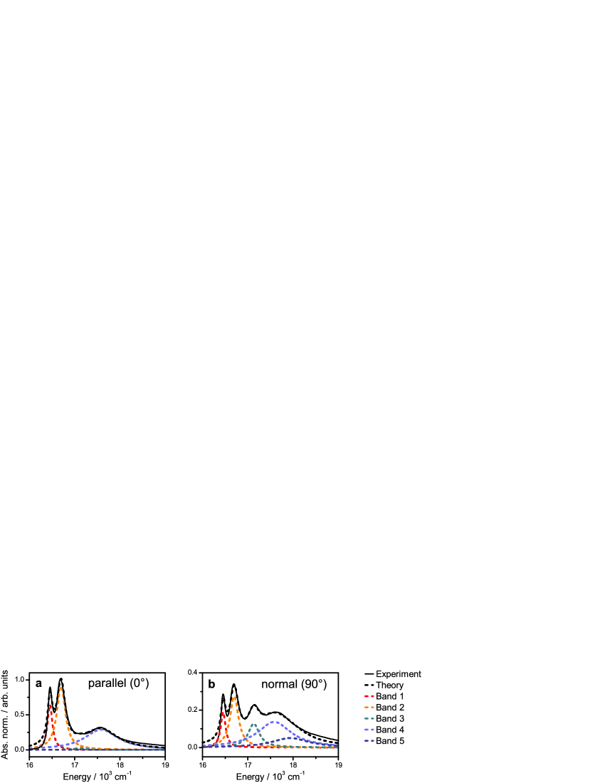
Figure 6: Absorption spectrum of C8O3. a, Absorption spectrum with light polarized parallel to the longitudinal axis of C8O3. Experimental and theoretical results are shown as a black solid line and a black dashed line, respectively. Theoretical results were modeled by a sum of Lorentzian functions, which describe bands 1-5 of C8O3. Each Lorentzian function is shown as a colored dashed line. b, Absorption spectrum with light polarized normal to the longitudinal axis of C8O3. Note that the vertical scales in a and b are different.

By fitting experimental 2D spectra to the theoretical prediction of N11 and R31, which will be discussed later, we found that $\hbar\Delta\Omega_{31}\approx 720\,{\rm cm^{-1}}$, $\hbar\nu_{1}\approx 668\,{\rm cm^{-1}}$, $\hbar\Gamma_{g1}\approx 65\,{\rm cm^{-1}}$, $\hbar\Gamma_{g3}\approx 150\,{\rm cm^{-1}}$, $\hbar\Gamma_{13}\approx 80\,{\rm cm}^{-1}$, $S_{1}=0.0006$ (cf. $\hbar\nu_{1}\sqrt{S_{1}}\approx 16\,{\rm cm}^{-1}$) and $\gamma_{v}\lesssim(1\,{\rm ps})^{-1}$. The estimated electronic decoherence rates $\Gamma_{g1}$ and $\Gamma_{g3}$ reproduce well the absorption spectrum of C8O3, as shown in Fig. 6, where experimental and theoretical results are shown as a black solid line and a black dashed line, respectively. The theoretical results were modeled by a sum of the Lorentzian functions with linewidths $2\Gamma_{gk}$ for $k\in\{1,2,3,4,5\}$, each of which describes the absorption of band $k$: each Lorentzian function is shown as a colored dashed line. The estimated values of the parameters lead to $\hbar\delta\omega\approx 1.6\,{\rm cm^{-1}}$ and $\hbar\delta\gamma\approx 2.1\,{\rm cm^{-1}}$, which are smaller than the experimental resolution of $\sim$$\,40\,{\rm cm}^{-1}$. This implies that for the case of C8O3, we can approximate $\Delta\Omega_{31}^{\prime}$ and $\nu_{1}^{\prime}$ by $\Delta\Omega_{31}$ and $\nu_{1}$, respectively, with $\delta\omega\approx 0$ and $\delta\gamma\approx 0$. More specifically, when the exciton-vibrational coupling is sufficiently small, such that $\nu_{1}\sqrt{S_{1}}<\left|i\Delta\nu_{1}-\Gamma_{13}\right|$ with $\Delta\nu_{1}=\Delta\Omega_{31}-\nu_{1}$, and the dissipation rate of the vibrational mode is negligible within the timescale of the total measurement time, i.e. $\gamma_{v}\approx 0$, the response function determining N11 in Eq. (28) is reduced to

$$R_{1g}(\omega_{1},t_{2},\omega_{3})\approx\mu_{1p}^{2}\mu_{3n}^{2}\frac{1}{i(\omega_{1}-\Omega_{1})-\Gamma_{g1}}\frac{1}{i(\omega_{3}-\Omega_{1})-\Gamma_{g1}}\left[e^{(i\Delta\Omega_{31}-\Gamma_{13})t_{2}}(1-\epsilon_{2}^{2})+e^{i\nu_{1}t_{2}}\epsilon_{2}^{2}\right],$$ (31)

with $\epsilon_{2}$ representing the degree of vibronic mixing during waiting time $t_{2}$

$$\epsilon_{2}=i\nu_{1}\sqrt{S_{1}}(i\Delta\nu_{1}-\Gamma_{13})^{-1},$$ (32)

where the vibronic eigenstates $\mathinner{\langle{\tilde{3}_{0}}|}$ and $\mathinner{\langle{\tilde{1}_{1}}|}$ are approximated by $\mathinner{\langle{\tilde{3}_{0}}|}\propto\left\langle{3_{0}}\right|+\epsilon_{2}\left\langle{1_{1}}\right|$ and $\mathinner{\langle{\tilde{1}_{1}}|}\propto\left\langle{1_{1}}\right|-\epsilon_{2}\left\langle{3_{0}}\right|$, respectively, with $|\epsilon_{2}|^{2}\ll 1$ (in the main text, $\epsilon_{2}$ was denoted by $\epsilon$ for the sake of simplicity). It can be seen in Eq. (32) that $|\epsilon_{2}|$ increases as the exciton-vibrational coupling $\nu_{1}\sqrt{S_{1}}$ increases or the detuning $|\Delta\nu_{1}|=|\Delta\Omega_{31}-\nu_{1}|$ between exciton splitting and vibrational frequency decreases. This implies that the vibronic mixing of the coherences $\left|{1_{0}}\right\rangle\left\langle{3_{0}}\right|$ and $\left|{1_{0}}\right\rangle\left\langle{1_{1}}\right|$ requires resonance between excitons and vibrations and induces the observed long-lived beating signal in N11. In this respect, when $|\epsilon_{2}|$ decreases as a result of a high electronic decoherence rate $\Gamma_{13}$, the coherence $\left|{1_{0}}\right\rangle\left\langle{3_{0}}\right|$ generated by the second pulse (see Fig. 5a) will decohere too quickly and thereby suppressing the vibronic mixing of $\left|{1_{0}}\right\rangle\left\langle{3_{0}}\right|$ and $\left|{1_{0}}\right\rangle\left\langle{1_{1}}\right|$ during waiting time $t_{2}$, which in turn will suppress the long-lived beating signal in N11. This is related to the fact that $\epsilon_{2}$ is proportional to the exciton-vibrational coupling $\nu_{1}\sqrt{S_{1}}$ and the amplitude of the long-lived component $e^{i\nu_{1}t_{2}}$ in Eq. (31) is proportional to $\epsilon_{2}^{2}$. As such, when $\nu_{1}\sqrt{S_{1}}<\left|i\Delta\nu_{1}-\Gamma_{13}\right|$, the response function for N11 can be effectively described by two transitions between $\left|{1_{0}}\right\rangle\left\langle{3_{0}}\right|$ and $\left|{1_{0}}\right\rangle\left\langle{1_{1}}\right|$ during waiting time $t_{2}$, mediated by exciton-vibrational coupling $\nu_{1}\sqrt{S_{1}}$, i.e. $\left|{1_{0}}\right\rangle\left\langle{3_{0}}\right|\rightarrow\left|{1_{0}}\right\rangle\left\langle{1_{1}}\right|\rightarrow\left|{1_{0}}\right\rangle\left\langle{3_{0}}\right|$, within the timescale of the electronic decoherence rate $\Gamma_{13}$, as shown in Fig. 5a. When the condition of $\nu_{1}\sqrt{S_{1}}<\left|i\Delta\nu_{1}-\Gamma_{13}\right|$ is not satisfied, the response function for N11 is represented by $R_{1g}(\omega_{1},t_{2},\omega_{3})=\sum_{n=0}^{\infty}h_{n}(\omega_{1},t_{2},\omega_{3})(i\nu_{1}\sqrt{S_{1}})^{2n}$ with the higher order terms proportional to $(i\nu_{1}\sqrt{S_{1}})^{2n}$, which describe multiple transitions between $\left|{1_{0}}\right\rangle\left\langle{3_{0}}\right|$ and $\left|{1_{0}}\right\rangle\left\langle{1_{1}}\right|$ during $t_{2}$.

In summary, when $\nu_{1}\sqrt{S_{1}}<\left|i\Delta\nu_{1}-\Gamma_{13}\right|$ and $\gamma_{v}\approx 0$, the response function for N11 at $(\omega_{1},\omega_{3})=(\Omega_{1},\Omega_{1})$ is given by

$$R_{1g}(t_{2})\approx\mu_{1p}^{2}\mu_{3n}^{2}\Gamma_{g1}^{-2}\left[e^{(i\Delta\Omega_{31}-\Gamma_{13})t_{2}}+e^{i\nu_{1}t_{2}}\epsilon_{2}^{2}\right],$$ (33)

with $\epsilon_{2}$ defined in Eq. (32). The lineshape of N11 is symmetric along $\omega_{1}$- and $\omega_{3}$-axes with a linewidth of $2\Gamma_{g1}$. These results are in line with the experimental observations shown in Figures 2 and 3 of the main text.

II.1.4 The response function for R31

Here we provide the response function for the beating signals in R31, which is the cross peak in the rephasing spectra centered at $(\omega_{1},\omega_{3})\approx(\Omega_{3},\Omega_{1})$. The response function for R31 can be derived using the same approach described above for N11. Here we provide the results without derivation. Figs. 5b-e show the Feynman diagrams contributing to the beating signals in R31. In Figs. 5b-d, the vibronic system is in the electronic excited states during $t_{2}$, while in Fig. 5e, the system is in the electronic ground state, each of which is called the stimulated emission (SE) and ground state bleaching (GSB) diagram, respectively.

When $\nu_{1}\sqrt{S_{1}}<\left|i\Delta\nu_{1}-\Gamma_{13}\right|$, $\nu_{1}\sqrt{S_{1}}<\left|i\Delta\nu_{1}+\Gamma_{g1}-\Gamma_{g3}\right|$ and $\gamma_{v}\approx 0$, which are satisfied for the case of C8O3, the contribution of the SE diagrams to R31 is approximated by

$$R_{2g}(\omega_{1},t_{2},\omega_{3}) \approx\mu_{1p}^{2}\mu_{3n}^{2}\left\{\frac{1}{-i(\omega_{1}-\Omega_{3})-\Gamma_{g3}}\frac{1}{i(\omega_{3}-\Omega_{1})-\Gamma_{g1}}\left[e^{(i\Delta\Omega_{31}-\Gamma_{13})t_{2}}(1-\epsilon_{2}^{2})+e^{i\nu_{1}t_{2}}\epsilon_{2}^{2}\right]\right.$$ (34)

$$\quad+\left(-\frac{1}{-i(\omega_{1}-\Omega_{3})-\Gamma_{g3}}+\frac{1}{-i(\omega_{1}-\Omega_{3}+\Delta\nu_{1})-\Gamma_{g1}}\right)\frac{1}{i(\omega_{3}-\Omega_{1})-\Gamma_{g1}}\left(-e^{(i\Delta\Omega_{31}-\Gamma_{13})t_{2}}+e^{i\nu_{1}t_{2}}\right)\epsilon_{1}\epsilon_{2}$$

$$\quad\left.+\left(-\frac{1}{-i(\omega_{1}-\Omega_{3})-\Gamma_{g3}}+\frac{1}{-i(\omega_{1}-\Omega_{3}+\Delta\nu_{1})-\Gamma_{g1}}\right)\frac{1}{i(\omega_{3}-\Omega_{1})-\Gamma_{g1}}e^{(i\Delta\Omega_{31}-\Gamma_{13})t_{2}}\epsilon_{1}^{2}\right\},$$

with $\epsilon_{1}$ representing the degree of vibronic mixing during coherence time $t_{1}$

$$\epsilon_{1}=i\nu_{1}\sqrt{S_{1}}(i\Delta\nu_{1}+\Gamma_{g1}-\Gamma_{g3})^{-1},$$ (35)

where $\Delta\Omega_{31}^{\prime}$ and $\nu_{1}^{\prime}$ are approximated by $\Delta\Omega_{31}$ and $\nu_{1}$, respectively. More specifically, $\epsilon_{1}$ is associated with the transition between $\left|{g_{0}}\right\rangle\left\langle{3_{0}}\right|$ and $\left|{g_{0}}\right\rangle\left\langle{1_{1}}\right|$ during $t_{1}$, while $\epsilon_{2}$ is associated with the transition between $\left|{1_{0}}\right\rangle\left\langle{3_{0}}\right|$ and $\left|{1_{0}}\right\rangle\left\langle{1_{1}}\right|$ during $t_{2}$. In Eq. (34), the first term proportional to $\epsilon_{2}^{2}$ describes the transition $\left|{1_{0}}\right\rangle\left\langle{3_{0}}\right|\rightarrow\left|{1_{0}}\right\rangle\left\langle{1_{1}}\right|\rightarrow\left|{1_{0}}\right\rangle\left\langle{3_{0}}\right|$ during $t_{2}$ (see Fig. 5b), the second term proportional to $\epsilon_{1}\epsilon_{2}$ describes the transition $\left|{g_{0}}\right\rangle\left\langle{3_{0}}\right|\rightarrow\left|{g_{0}}\right\rangle\left\langle{1_{1}}\right|$ during $t_{1}$ and the subsequent transition $\left|{1_{0}}\right\rangle\left\langle{1_{1}}\right|\rightarrow\left|{1_{0}}\right\rangle\left\langle{3_{0}}\right|$ during $t_{2}$ (see Fig. 5c), and the last term proportional to $\epsilon_{1}^{2}$ describes the transition $\left|{g_{0}}\right\rangle\left\langle{3_{0}}\right|\rightarrow\left|{g_{0}}\right\rangle\left\langle{1_{1}}\right|\rightarrow\left|{g_{0}}\right\rangle\left\langle{3_{0}}\right|$ during $t_{1}$ (see Fig. 5d). In the second and last terms, the lineshape function along the $\omega_{1}$-axis contains $(-i(\omega_{1}-\Omega_{3}+\Delta\nu_{1})-\Gamma_{g1})^{-1}$, which describes the presence of a sub-peak centered at $\omega_{1}=\Omega_{3}-\Delta\nu_{1}=\Omega_{1}+\nu_{1}<\Omega_{3}$ with a linewidth of $2\Gamma_{g1}$, which is induced by exciton-vibrational coupling. However, due to the condition of $|\epsilon_{1}|^{2}\ll 1$ and $|\epsilon_{2}|^{2}\ll 1$, the first term in Eq. (34) determines the overall lineshape of R31, which is given by $(-i(\omega_{1}-\Omega_{3})-\Gamma_{g3})^{-1}(i(\omega_{3}-\Omega_{1})-\Gamma_{g1})^{-1}$ that is centered at $(\omega_{1},\omega_{3})=(\Omega_{3},\Omega_{1})$ with the asymmetric linewidths of $2\Gamma_{g3}$ and $2\Gamma_{g1}$ along $\omega_{1}$- and $\omega_{3}$-axes, respectively.

The contribution of the GSB diagram to R31, with ground state coherence Jonas_PNAS2012_SI during $t_{2}$, is given by

$$R_{3g}(\omega_{1},t_{2},\omega_{3})\approx\left(\frac{1}{-i(\omega_{1}-\Omega_{3})-\Gamma_{g3}}-\frac{1}{-i(\omega_{1}-\Omega_{3}+\Delta\nu_{1})-\Gamma_{g1}}\right)\left(\frac{1}{i(\omega_{3}-\Omega_{1}-\Delta\nu_{1})-\Gamma_{g3}}-\frac{1}{i(\omega_{3}-\Omega_{1})-\Gamma_{g1}}\right)e^{i\nu_{1}t_{2}}\epsilon_{1}\epsilon_{3},$$ (36)

with $\epsilon_{3}$ representing the vibronic mixing during $t_{3}$

$$\epsilon_{3}=-i\nu_{1}\sqrt{S_{1}}(-i\Delta\nu_{1}+\Gamma_{g1}-\Gamma_{g3})^{-1},$$ (37)

which is associated with the transition $\left|{3_{0}}\right\rangle\left\langle{g_{1}}\right|\rightarrow\left|{1_{1}}\right\rangle\left\langle{g_{1}}\right|$ during $t_{3}$ shown in Fig. 5e. Here the vibrational frequency $\nu_{1}$ in $e^{i\nu_{1}t_{2}}$ stems from the vibrational coherence $\left|{g_{0}}\right\rangle\left\langle{g_{1}}\right|$ in the electronic ground-state manifold and not the result of the approximation $\delta\omega\approx 0$.

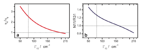
Figure 7: Long-lived beating signals in N11 and R31. a, The ratio $|\eta_{e}/\eta_{g}|$ between the contributions of the vibronic and vibrational coherences to the long-lived beating signal in R31. For the experimentally estimated value of $\Gamma_{13}$, marked by a vertical dashed line, the contribution of the vibronic coherence is greater than the vibrational coherence. b, The ratio $\Gamma_{g3}(\Gamma_{g1}|\eta_{e}-\eta_{g}|)^{-1}$ between the amplitudes of the long-lived beating signals in N11 ($\propto\Gamma_{g1}^{-2}$) and R31 ($\propto\Gamma_{g3}^{-1}\Gamma_{g1}^{-1}|\eta_{e}-\eta_{g}|$). In both a and b, we take the values of the parameters estimated from experimental results. According to Eq. (19), $\hbar(\Gamma_{g1}+\Gamma_{g3})\approx 215\,{\rm cm}^{-1}$ is the theoretical upper bound for $\Gamma_{13}$.

In summary, when $\nu_{1}\sqrt{S_{1}}<\left|i\Delta\nu_{1}-\Gamma_{13}\right|$, $\nu_{1}\sqrt{S_{1}}<\mathinner{|i\Delta\nu_{1}+\Gamma_{g1}-\Gamma_{g3}|}$ and $\gamma_{v}\approx 0$, the response function for R31 at $(\omega_{1},\omega_{3})=(\Omega_{3},\Omega_{1})$ is given by

$$R_{2g}(t_{2})+R_{3g}(t_{2})\approx\mu_{1p}^{2}\mu_{3n}^{2}\Gamma_{g3}^{-1}\Gamma_{g1}^{-1}[e^{(i\Delta\Omega_{31}-\Gamma_{13})t_{2}}+e^{i\nu_{1}t_{2}}\epsilon_{2}^{2}(\eta_{e}-\eta_{g})],$$ (38)

where $\eta_{e}=(\Gamma_{g1}+\Gamma_{13})(\Gamma_{g1}+i\Delta\nu_{1})^{-1}$ stems from the SE diagrams shown in Figs. 5b-d, while $\eta_{g}=(\Gamma_{13}-i\Delta\nu_{1})^{2}(\Gamma_{g1}+i\Delta\nu_{1})^{-1}(\Gamma_{g3}+i\Delta\nu_{1})^{-1}$ originates from the GSB diagram shown in Fig. 5e. It is interesting to note that the origin of the long-lived oscillations at R31, whether predominantly vibrational or vibronic, depends upon the electronic decoherence rates $\{\Gamma_{g1},\Gamma_{g3},\Gamma_{13}\}$ and detuning $\Delta\nu_{1}=\Delta\Omega_{31}-\nu_{1}$. In Fig. 7a, the ratio $|\eta_{e}/\eta_{g}|$ between the contributions of the vibronic and vibrational coherences to the long-lived beating signal in R31 is displayed as a function of the inter-exciton decoherence rate $\Gamma_{13}$, where $\{\Gamma_{g1},\Gamma_{g3},\Delta\nu_{1}\}$ are taken to be the values estimated from experimental results. Here $|\eta_{e}/\eta_{g}|>1$ implies that the long-lived beating signal in R31 is dominated by the vibronic coherence $\left|{1}\right\rangle\mathinner{\langle\tilde{1}_{1}|}$ in the electronic excited-state manifold. By fitting the experimentally measured beating signals in N11 and R31 to the theoretical model, we found that $\hbar\Gamma_{13}\approx 80\,{\rm cm}^{-1}$, which is marked by a vertical dashed line in Fig. 7a, where the contribution of the vibronic coherence is $\sim$$\,2.5$ times greater than the vibrational coherence. These results imply that the long-lived beating signal in R31 is dominated by vibronic coherence, originating from electronic excited states. It is notable that the vibronic contribution outweighs the vibrational part for a wide range of $\Gamma_{13}$. This is mainly due to the fact that the vibronic mixing $\epsilon_{2}\propto(i\Delta\nu_{1}-\Gamma_{13})^{-1}$ during $t_{2}$ depends on the inter-exciton decoherence rate $\Gamma_{13}$, while the other vibronic mixings $\epsilon_{1}\propto(i\Delta\nu_{1}+\Gamma_{g1}-\Gamma_{g3})^{-1}$ and $\epsilon_{3}\propto(-i\Delta\nu_{1}+\Gamma_{g1}-\Gamma_{g3})^{-1}$ during $t_{1}$ and $t_{3}$ are independent of $\Gamma_{13}$. Considering that vibronic coherence depends on $\epsilon_{2}$ (see Eq. (34) and Figs. 5b and c), while vibrational coherence depends on $\epsilon_{1}\epsilon_{3}$ (see Eq. (36) and Fig. 5e), the vibronic contribution is increased as $\Gamma_{13}$ decreases. We note that these results are in line with the experimental observation that the amplitude of the long-lived beating signal in N11 is greater than that of R31 (see Figures 3b and c in the main text). In Fig. 7b, the ratio $\Gamma_{g3}(\Gamma_{g1}|\eta_{e}-\eta_{g}|)^{-1}$ between the amplitudes of the long-lived beating signals in N11 and R31 is displayed as a function of the inter-exciton decoherence rate $\Gamma_{13}$. Here the amplitude of the long-lived beating signal in N11 is greater than R31, i.e. $\Gamma_{g3}(\Gamma_{g1}|\eta_{e}-\eta_{g}|)^{-1}>1$, for a range of $\Gamma_{13}$ where the vibronic coherence dominates the long-lived beating signal in R31, as shown in Fig. 7a.

II.1.5 Numerical simulation of N11 and R31

So far the analytic form of the response functions for N11 and R31 were derived with the assumption that the vibronic system is well described within the subspace of the vibrational ground and first excited states, which is valid for a small Huang-Rhys factor $S_{1}$. To clarify the validity of this assumption, we performed numerical simulation of the beating signals in N11 and R31 with higher vibrational excited states, i.e. $\{\left|{g_{0}}\right\rangle,\left|{g_{1}}\right\rangle,\cdots,\left|{g_{n}}\right\rangle,\left|{1_{0}}\right\rangle,\left|{1_{1}}\right\rangle,\cdots,\left|{1_{n}}\right\rangle,\left|{3_{0}}\right\rangle,\left|{3_{1}}\right\rangle,\cdots,\left|{3_{n}}\right\rangle\}$ with $n\geq 1$. We found that the theoretical beating signals converge for $n\geq 1$ and the numerical results are well matched to the analytical results. Here the electronic decoherence was modeled by a convex combination of two effective dissipators, i.e. $p{\cal D}_{1}[\rho(t)]+(1-p){\cal D}_{2}[\rho(t)]$ with $0\leq p\leq 1$, where the dissipators are given by

$${\cal D}_{1}[\rho(t)] =\Gamma_{g1}(2\left|{1}\right\rangle\left\langle{1}\right|\rho(t)\left|{1}\right\rangle\left\langle{1}\right|-\{\left|{1}\right\rangle\left\langle{1}\right|,\rho(t)\})+\Gamma_{g3}(2\left|{3}\right\rangle\left\langle{3}\right|\rho(t)\left|{3}\right\rangle\left\langle{3}\right|-\{\left|{3}\right\rangle\left\langle{3}\right|,\rho(t)\}),$$ (39)

$${\cal D}_{2}[\rho(t)] =2\left(\sqrt{\Gamma_{g1}}\left|{1}\right\rangle\left\langle{1}\right|+\sqrt{\Gamma_{g3}}\left|{3}\right\rangle\left\langle{3}\right|\,\right)\rho(t)\left(\sqrt{\Gamma_{g1}}\left|{1}\right\rangle\left\langle{1}\right|+\sqrt{\Gamma_{g3}}\left|{3}\right\rangle\left\langle{3}\right|\,\right)-\{\Gamma_{g1}\left|{1}\right\rangle\left\langle{1}\right|+\Gamma_{g3}\left|{3}\right\rangle\left\langle{3}\right|,\rho(t)\}.$$ (40)

By substituting electronic coherences $\left|{g}\right\rangle\left\langle{1}\right|$ and $\left|{g}\right\rangle\left\langle{3}\right|$ to the dissipators, one can show that both ${\cal D}_{1}[\rho(t)]$ and ${\cal D}_{2}[\rho(t)]$ give rise to the same set of decoherence rates $\Gamma_{g1}$ and $\Gamma_{g3}$ for $\left|{g}\right\rangle\left\langle{1}\right|$ and $\left|{g}\right\rangle\left\langle{3}\right|$, respectively, implying that the decoherence rates of $\left|{g}\right\rangle\left\langle{1}\right|$ and $\left|{g}\right\rangle\left\langle{3}\right|$ are independent of the value of $p$ in the convex combination. For $\left|{1}\right\rangle\left\langle{3}\right|$, on the other hand, ${\cal D}_{1}[\rho(t)]$ and ${\cal D}_{2}[\rho(t)]$ lead to different decoherence rates $\Gamma_{g1}+\Gamma_{g3}$ and $(\sqrt{\Gamma_{g1}}-\sqrt{\Gamma_{g3}}~{})^{2}$, respectively. This enables us to vary the inter-exciton decoherence rate $\Gamma_{13}$ within a range of $(\sqrt{\Gamma_{g1}}-\sqrt{\Gamma_{g3}}~{})^{2}\leq\Gamma_{13}\leq\Gamma_{g1}+\Gamma_{g3}$ by changing the value of $p$ in the convex combination. In addition to the electronic decoherence, the relaxation of the vibrational mode was modeled by Eq. (20) in the simulations. We found that Eq. (20) can be approximated by Eq. (21) due to the high vibrational frequency ($\hbar\nu_{1}\gg k_{B}T$).

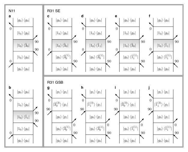
Figure 8: Feynman diagrams contributing to the beating signals in N11 and R31 represented in vibronic eigenbasis. a,b, The stimulated emission diagrams contributing to the beating signals in N11. c-f, The stimulated emission diagrams contributing to the beating signals in R31. g-j, The ground state bleaching diagrams contributing to the beating signals in R31.

II.1.6 Feynman diagrams represented in vibronic eigenbasis

Here we provide the Feynman diagrams for N11 and R31 represented in the vibronic eigenbasis of the time evolution super-operator ${\cal U}(t)$, which are equivalent to the Feynman diagrams in the uncoupled state basis shown in Fig. 5.

For N11, the vibronic mixing $\epsilon_{2}$ takes place during waiting time $t_{2}$ (cf. Fig. 5a), where the vibronic coherences responsible for the short-lived and long-lived beating signals in N11 are given by

$$\left|{1_{0}}\right\rangle\mathinner{\langle\tilde{3}_{0}|} =(1+\epsilon_{2}^{2})^{-1/2}(\left|{1_{0}}\right\rangle\left\langle{3_{0}}\right|+\epsilon_{2}\left|{1_{0}}\right\rangle\left\langle{1_{1}}\right|),$$ (41)

$$\left|{1_{0}}\right\rangle\mathinner{\langle\tilde{1}_{1}|} =(1+\epsilon_{2}^{2})^{-1/2}(\left|{1_{0}}\right\rangle\left\langle{1_{1}}\right|-\epsilon_{2}\left|{1_{0}}\right\rangle\left\langle{3_{0}}\right|),$$ (42)

respectively, where the vibronic eigenstates $\mathinner{\langle\tilde{3}_{0}|}\propto\left\langle{3_{0}}\right|+\epsilon_{2}\left\langle{1_{1}}\right|$ and $\mathinner{\langle\tilde{1}_{1}|}\propto\left\langle{1_{1}}\right|-\epsilon_{2}\left\langle{3_{0}}\right|$ are normalized by $(1+\epsilon_{2}^{2})^{-1/2}$, not by $(1+|\epsilon_{2}|^{2})^{-1/2}$, due to the biorthogonality of the eigenstates of the non-Hermitian operator $K$ in Eq. (25). When the light-induced vibrational excitation of overtones, i.e. $\left\langle{1_{1}}\right|$, is negligible due to the small Franck-Condon factors, the transition dipole moments of the vibronic eigenstates $\mathinner{\langle\tilde{3}_{0}|}$ and $\mathinner{\langle\tilde{1}_{1}|}$ are determined by their amplitudes in $\left\langle{3_{0}}\right|$, each of which is given by $\mu_{3n}(1+\epsilon_{2}^{2})^{-1/2}$ and $-\mu_{3n}(1+\epsilon_{2}^{2})^{-1/2}\epsilon_{2}$, respectively. Here $\mu_{3n}$ denotes the transition dipole moment of $\left\langle{3_{0}}\right|$. In the eigenbasis, the Feynman diagrams responsible for the short-lived and long-lived beating signals in N11 are described by Figs. 8a and b, respectively. Given that there are two transitions between $\left\langle{g_{0}}\right|$ and $\mathinner{\langle\tilde{3}_{0}|}$ (and also between $\left\langle{g_{0}}\right|$ and $\mathinner{\langle\tilde{1}_{1}|}$) by the second and third pulses, the square of the transition dipole moments of $\mathinner{\langle\tilde{3}_{0}|}$ and $\mathinner{\langle\tilde{1}_{1}|}$ is reflected in the response function, each of which is given by $\mu_{3n}^{2}(1+\epsilon_{2}^{2})^{-1}\approx\mu_{3n}^{2}(1-\epsilon_{2}^{2})$ and $\mu_{3n}^{2}\epsilon_{2}^{2}$, respectively. This is in line with the analytic form of the response function for N11 shown in Eq. (31).

For R31, on the other hand, vibronic mixing takes place during coherence, waiting and rephasing times ($t_{1}$, $t_{2}$, $t_{3}$, respectively, cf. Figs. 5b-e). The vibronic mixing $\epsilon_{1}$ during coherence time $t_{1}$ leads to the vibronic eigenstates $\mathinner{\langle\tilde{3}_{0}^{(1)}|}\propto\left\langle{3_{0}}\right|+\epsilon_{1}\left\langle{1_{1}}\right|$ and $\mathinner{\langle\tilde{1}_{1}^{(1)}|}\propto\left\langle{1_{1}}\right|-\epsilon_{1}\left\langle{3_{0}}\right|$, where vibronic coherences during $t_{1}$ are represented by

$$\left|{g_{0}}\right\rangle\mathinner{\langle\tilde{3}_{0}^{(1)}|} =(1+\epsilon_{1}^{2})^{-1/2}(\left|{g_{0}}\right\rangle\left\langle{3_{0}}\right|+\epsilon_{1}\left|{g_{0}}\right\rangle\left\langle{1_{1}}\right|),$$ (43)

$$\left|{g_{0}}\right\rangle\mathinner{\langle\tilde{1}_{1}^{(1)}|} =(1+\epsilon_{1}^{2})^{-1/2}(\left|{g_{0}}\right\rangle\left\langle{1_{1}}\right|-\epsilon_{1}\left|{g_{0}}\right\rangle\left\langle{3_{0}}\right|).$$ (44)

Here the superindex $(1)$ of $\mathinner{\langle\tilde{3}_{0}^{(1)}|}$ and $\mathinner{\langle\tilde{1}_{1}^{(1)}|}$ reminds us that the vibronic mixing takes place during coherence time $t_{1}$: throughout this work, the vibronic eigenstates $\mathinner{\langle\tilde{3}_{0}^{(2)}|}$ and $\mathinner{\langle\tilde{1}_{1}^{(2)}|}$ responsible for the vibronic mixing $\epsilon_{2}$ during waiting time $t_{2}$ have, for the sake of simplicity, been denoted by $\mathinner{\langle\tilde{3}_{0}|}$ and $\mathinner{\langle\tilde{1}_{1}|}$, respectively. We note that $\epsilon_{1}$ in Eq. (35) is different from $\epsilon_{2}$ in Eq. (32), as the time evolution of the coherences $\left|{g_{0}}\right\rangle\left\langle{3_{0}}\right|$ and $\left|{g_{0}}\right\rangle\left\langle{1_{1}}\right|$ during coherence time $t_{1}$ is governed by a different non-Hermitian operator $K_{1}$

$$K_{1}=(i\Omega_{3}-\Gamma_{g3})\left|{3_{0}}\right\rangle\left\langle{3_{0}}\right|+(i\Omega_{1}+i\nu_{1}-\Gamma_{g1}-\gamma_{v})\left|{1_{1}}\right\rangle\left\langle{1_{1}}\right|+i\nu_{1}\sqrt{S_{1}}(\left|{3_{0}}\right\rangle\left\langle{1_{1}}\right|+\left|{1_{1}}\right\rangle\left\langle{3_{0}}\right|),$$ (45)

defined by ${\cal U}(t_{1})\left|{g_{0}}\right\rangle\left\langle{3_{0}}\right|=\left|{g_{0}}\right\rangle\left\langle{3_{0}}\right|e^{K_{1}t_{1}}$. In the eigenbasis, the SE diagrams shown in Figs. 5b-d can be represented by four diagrams shown in Figs. 8c-f, where the transition dipole moments of $\mathinner{\langle\tilde{3}_{0}^{(1)}|}$ and $\mathinner{\langle\tilde{1}_{1}^{(1)}|}$ are given by $\mu_{3n}(1+\epsilon_{1}^{2})^{-1/2}$ and $-\mu_{3n}(1+\epsilon_{1}^{2})^{-1/2}\epsilon_{1}$, respectively. It is notable that the vibronic eigenstates $\mathinner{\langle\tilde{3}_{0}^{(1)}|}$ and $\mathinner{\langle\tilde{1}_{1}^{(1)}|}$ during coherence time $t_{1}$ are different from the vibronic eigenstates $\mathinner{\langle\tilde{3}_{0}|}$ and $\mathinner{\langle\tilde{1}_{1}|}$ during waiting time $t_{2}$, as the vibronic system is in a superposition between electronic ground and excited states (see Eqs. (43) and (44)) and in the electronic excited-state manifold (see Eqs. (41) and (42)), respectively, which leads in general to different values of the vibronic mixings $\epsilon_{1}$ and $\epsilon_{2}$. The diagrams shown in Figs. 8c-f describe the fact that the vibronic eigenstates $\mathinner{\langle\tilde{3}_{0}^{(1)}|}$ and $\mathinner{\langle\tilde{1}_{1}^{(1)}|}$ can be represented by superpositions of $\mathinner{\langle\tilde{3}_{0}|}$ and $\mathinner{\langle\tilde{1}_{1}|}$. In Figs. 8c and d, for instance, the vibronic eigenstate $\mathinner{\langle\tilde{3}_{0}^{(1)}|}$ induced by the first pulse can be represented by a superposition of $\mathinner{\langle\tilde{3}_{0}|}$ and $\mathinner{\langle\tilde{1}_{1}|}$

$$\mathinner{\langle\tilde{3}_{0}^{(1)}|} =(1+\epsilon_{1}^{2})^{-1/2}(\left\langle{3_{0}}\right|+\epsilon_{1}\left\langle{1_{1}}\right|)$$ (46)

$$=(1+\epsilon_{1}^{2})^{-1/2}(1+\epsilon_{2}^{2})^{-1/2}[(1+\epsilon_{1}\epsilon_{2})\mathinner{\langle\tilde{3}_{0}|}+(\epsilon_{1}-\epsilon_{2})\mathinner{\langle\tilde{1}_{1}|})].$$ (47)

Here the prefactors of $\mathinner{\langle\tilde{3}_{0}|}$ and $\mathinner{\langle\tilde{1}_{1}|}$, i.e. $(1+\epsilon_{1}^{2})^{-1/2}(1+\epsilon_{2}^{2})^{-1/2}(1+\epsilon_{1}\epsilon_{2})$ and $(1+\epsilon_{1}^{2})^{-1/2}(1+\epsilon_{2}^{2})^{-1/2}(\epsilon_{1}-\epsilon_{2})$, enable us to introduce two separated diagrams shown in Figs. 8c and d, where the prefactors are multiplied to the response function, similar to the transition dipole moment. Similarly, the other vibronic eigenstate $\mathinner{\langle\tilde{1}_{1}^{(1)}|}$ can be represented by a superposition of $\mathinner{\langle\tilde{3}_{0}|}$ and $\mathinner{\langle\tilde{1}_{1}|}$, leading to the prefactors for the diagrams shown in Figs. 8e and f. Using the transition dipole moments of $\mathinner{\langle\tilde{3}_{0}|}$ and $\mathinner{\langle\tilde{1}_{1}|}$ induced by the third pulse, one can show that the response function induced by the SE diagrams is given by Eq. (34): here the lineshape functions $(-i(\omega_{1}-\Omega_{3})-\Gamma_{g3})^{-1}$ and $(-i(\omega_{1}-\Omega_{3}+\Delta\nu_{1})-\Gamma_{g1})^{-1}$ along the $\omega_{1}$-axis correspond to the diagrams where the vibronic system is in $\left|{g_{0}}\right\rangle\mathinner{\langle\tilde{3}_{0}^{(1)}|}$ (cf. Figs. 8c and d) and in $\left|{g_{0}}\right\rangle\mathinner{\langle\tilde{1}_{1}^{(1)}|}$ (cf. Figs. 8e and f), respectively, during coherence time $t_{1}$.

The vibronic mixing $\epsilon_{3}$ during rephasing time $t_{3}$ leads to the vibronic eigenstates $\mathinner{|\tilde{3}_{0}^{(3)}\rangle}\propto\left|{3_{0}}\right\rangle+\epsilon_{3}\left|{1_{1}}\right\rangle$ and $\mathinner{|\tilde{1}_{1}^{(3)}\rangle}\propto\left|{1_{1}}\right\rangle-\epsilon_{3}\left|{3_{0}}\right\rangle$, where vibronic coherences during $t_{3}$ are represented by

$$\mathinner{|\tilde{3}_{0}^{(3)}\rangle}\left\langle{g_{1}}\right| =(1+\epsilon_{3}^{2})^{-1/2}(\left|{3_{0}}\right\rangle\left\langle{g_{1}}\right|+\epsilon_{3}\left|{1_{1}}\right\rangle\left\langle{g_{1}}\right|),$$ (48)

$$\mathinner{|\tilde{1}_{1}^{(3)}\rangle}\left\langle{g_{1}}\right| =(1+\epsilon_{3}^{2})^{-1/2}(\left|{1_{1}}\right\rangle\left\langle{g_{1}}\right|-\epsilon_{3}\left|{3_{0}}\right\rangle\left\langle{g_{1}}\right|).$$ (49)

The time evolution of the coherences $\left|{3_{0}}\right\rangle\left\langle{g_{1}}\right|$ and $\left|{1_{1}}\right\rangle\left\langle{g_{1}}\right|$ is governed by a non-Hermitian operator $K_{3}$

$$K_{3}=(-i\Omega_{3}+i\nu_{1}-\Gamma_{g3}-\gamma_{v})\left|{3_{0}}\right\rangle\left\langle{3_{0}}\right|+(-i\Omega_{1}-\Gamma_{g1})\left|{1_{1}}\right\rangle\left\langle{1_{1}}\right|-i\nu_{1}\sqrt{S_{1}}(\left|{3_{0}}\right\rangle\left\langle{1_{1}}\right|+\left|{1_{1}}\right\rangle\left\langle{3_{0}}\right|),$$ (50)

defined by ${\cal U}(t_{3})\left|{3_{0}}\right\rangle\left\langle{g_{1}}\right|=e^{K_{3}t_{3}}\left|{3_{0}}\right\rangle\left\langle{g_{1}}\right|$. Similar to the SE diagrams, the GSB diagram shown in Fig. 5e can be represented by four diagrams shown in Figs. 8g-j. Using the transition dipole moments of the vibronic eigenstates, one can show that the response function induced by the GSB diagrams is given by Eq. (36), where the lineshape functions $(i(\omega_{3}-\Omega_{1}-\Delta\nu_{1})-\Gamma_{g3})^{-1}$ and $(i(\omega_{3}-\Omega_{1})-\Gamma_{g1})^{-1}$ along the $\omega_{3}$-axis correspond to the diagrams where the vibronic system is in $\mathinner{|\tilde{3}_{0}^{(3)}\rangle}\left\langle{g_{1}}\right|$ and in $\mathinner{|\tilde{1}_{1}^{(3)}\rangle}\left\langle{g_{1}}\right|$, respectively, during $t_{3}$.

These results imply that the Feynman diagrams for N11 and R31 can be represented in both uncoupled state basis and vibronic eigenbasis equivalently, and the analytic form of the response functions in Eqs. (31), (34) and (36) is independent of the basis chosen to represent the Feynman diagrams.

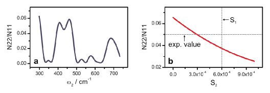
Figure 9: The relative amplitude of N22 and N11. a, The absolute square of the Fourier transform of the beating signal in N22 as a function of $\omega_{2}$, which is normalized to the amplitude of N11 at $\hbar\omega_{2}\approx 705\,{\rm cm}^{-1}$. b, Theoretical results of the ratio between N22 and N11 are displayed as a function of the Huang-Rhys factor $S_{2}$. The Huang-Rhys factor $S_{1}=0.0006$ of the vibrational mode with frequency $\hbar\nu_{1}\approx 668\,{\rm cm}^{-1}$ is marked by a vertical dashed line.

II.2 The response function for N22

Here we provide a vibronic model for bands 2 and 3 of C8O3, where bands 2 and 3 are coupled to the intramolecular vibrational modes with frequency $\hbar\nu_{2}\approx 470\,{\rm cm}^{-1}$.

In Fig. 9a, the absolute square of the Fourier transform of the beating signal in N22 is displayed as a function of $\omega_{2}$, which is normalized by the amplitude of N11 at $\hbar\omega_{2}\approx 705\,{\rm cm}^{-1}$. The amplitude of N22 is maximized around $\hbar\omega_{2}\approx 460\,{\rm cm}^{-1}$ with an amplitude in the range of $5\,\%$ of the N11 peak. When bands 2 and 3 are coupled to a vibrational mode with frequency $\nu_{2}$ mediated by an effective Huang-Rhys factor $S_{2}$, the response function for N22 is given by

$$R_{1g}(t_{2})\approx\mu_{2p}^{2}\mu_{3n}^{2}\Gamma_{g2}^{-2}\left[e^{(i\Delta\Omega_{32}-\Gamma_{23})t_{2}}+e^{i\nu_{2}t_{2}}\left(\frac{i\nu_{2}\sqrt{S_{2}}}{i\Delta\nu_{2}-\Gamma_{23}}\right)^{2}\right],$$ (51)

with $\Delta\nu_{2}=\Delta\Omega_{32}-\nu_{2}$, $\mu_{2p}$ denotes the transition dipole moment of band 2 for light polarized parallel to the longitudinal axis of C8O3 and $\hbar\Gamma_{g2}\approx 110\,{\rm cm}^{-1}$ represents the electronic decoherence rate of band 2, both of which can be estimated using the absorption spectrum shown in Fig. 6. From the experimentally measured beating signal in N22, we found that $\hbar\Gamma_{23}\approx 200\,{\rm cm}^{-1}<\hbar(\Gamma_{g2}+\Gamma_{g3})$ (not shown). In Fig. 9b, the amplitude of the theoretical N22 is displayed as a function of the Huang-Rhys factor $S_{2}$, which is about $5\,\%$ of N11 over a range of realistic $S_{2}$ values. For a comparison, the Huang-Rhys factor $S_{1}$ of the vibrational mode with frequency $\hbar\nu_{1}\approx 668\,{\rm cm}^{-1}$ is marked by a vertical dashed line. These results imply that the small amplitude of the beating signal in N22 is mainly due to the high electronic decoherence rate of band 2.

II.3 A correlated fluctuation model for bands 1 and 3 of C8O3

Here we provide a correlated fluctuation model for bands 1 and 3 of C8O3 where coherent interaction between excitons and quasi-resonant vibrations is not considered. Within the level of Markovian quantum master equations, we show that the experimentally measured long-lived beating signals in N11 and R31 cannot be explained by correlated fluctuations.

The main idea of the correlated fluctuations is that when bands 1 and 3 are coupled to a common environment, the correlated noise enables the inter-exciton coherence $\left|{1}\right\rangle\left\langle{3}\right|$ to decohere very slowly compared to the coherences $\left|{g}\right\rangle\left\langle{1}\right|$ and $\left|{g}\right\rangle\left\langle{3}\right|$ between electronic ground state and excitons. This is similar in spirit to the decoherence-free subspaces in quantum information theoryWhaley_PRL1998_SI . Here we consider a Markovian quantum master equation in the form of

$$\frac{d}{dt}\rho(t)=-\frac{i}{\hbar}[\tilde{H}_{e},\rho(t)]+\sum_{\omega}\sum_{\alpha,\beta}\gamma_{\alpha\beta}(\omega)\left(A_{\beta}(\omega)\rho(t)A_{\alpha}^{\dagger}(\omega)-\frac{1}{2}\{A_{\alpha}^{\dagger}(\omega)A_{\beta}(\omega),\rho(t)\}\right),$$ (52)

which is the same to Eq. (3.143) in The Theory of Open Quantum Systems by H.-P. Breuer and F. PetruccioneBreuer_SI , which is called the Redfield equation with the secular approximation in some literatureRebentrost_JPCB2009_SI . Here the interaction Hamiltonian is modeled by $H_{e-{\rm ph}}=\sum_{\alpha}A_{\alpha}\otimes B_{\alpha}$ with $A_{\alpha}=A_{\alpha}^{\dagger}$ and $B_{\alpha}=B_{\alpha}^{\dagger}$, each of which is a Hermitian operator of the system and environmental degrees of freedom, respectively. With the exciton states $\left|{k}\right\rangle$ defined by $\tilde{H}_{e}\left|{k}\right\rangle=\hbar\Omega_{k}\left|{k}\right\rangle$, we introduce a projection operator $\Pi(\Omega)=\sum_{\Omega=\Omega_{k}}\left|{k}\right\rangle\left\langle{k}\right|=\sum_{k}\delta(\Omega,\Omega_{k})\left|{k}\right\rangle\left\langle{k}\right|$ where the Kronecker delta is defined by $\delta(i,j)=1$ if $i=j$ and $\delta(i,j)=0$ otherwise. In other words, $\Pi(\Omega)$ is a projection operator onto the exciton subspace belonging to the exciton energy $\Omega$. In Eq. (52), $A_{\alpha}(\omega)=\sum_{\Omega^{\prime}-\Omega=\omega}\Pi(\Omega)A_{\alpha}\Pi(\Omega^{\prime})=\sum_{\Omega,\Omega^{\prime}}\delta(\omega,\Omega^{\prime}-\Omega)\Pi(\Omega)A_{\alpha}\Pi(\Omega^{\prime})$. The interaction Hamiltonian $H_{e-{\rm ph}}$ between excitons and background phonons is modeled by $A_{\alpha}=\left|{e_{\alpha}}\right\rangle\left\langle{e_{\alpha}}\right|$ and $B_{\alpha}=\sum_{\xi}\hbar g_{\alpha\xi}(a_{\xi}^{\dagger}+a_{\xi})$, where $g_{\alpha\xi}$ denotes the coupling of the local excitation of site $\alpha$ to a background phonon mode $\xi$. When $g_{\alpha\xi}\neq 0$ and $g_{\beta\xi}\neq 0$ for different $\alpha$ and $\beta$, spatially separated sites $\alpha$ and $\beta$ are coupled to a common phonon mode $\xi$, leading to correlated fluctuations in the energy levels of the different sites $\alpha$ and $\beta$. The correlated fluctuations are absent when each site is coupled to an independent phonon bath, such that $g_{\alpha\xi}g_{\beta\xi}=0$ for all $\alpha\neq\beta$ and $\xi$. The information of the correlated fluctuations is included in the definition of $\gamma_{\alpha\beta}(\omega)$ in Eq. (52)

$$\gamma_{\alpha\beta}(\omega)=\frac{1}{\hbar^{2}}\int_{-\infty}^{\infty}dse^{i\omega s}\mathinner{\langle B_{\alpha}^{\dagger}(s)B_{\beta}(0)\rangle},$$ (53)

where for fixed $\omega$, $\gamma_{\alpha\beta}(\omega)$ form a positive matrixBreuer_SI . Here $\gamma_{\alpha\beta}(\omega)=0$ for all $\alpha\neq\beta$ if each site is coupled to an independent phonon bath and $\gamma_{\alpha\beta}(\omega)\neq 0$ for some $\alpha\neq\beta$ if different sites $\alpha$ and $\beta$ are coupled to the same phonon modes.

Using experimentally measured absorption and 2D spectra of C8O3, we found that the electronic decoherence rate $\Gamma_{gk}$ of the coherence $\left|{g}\right\rangle\left\langle{k}\right|$ between electronic ground state and band $k$ is given by $\hbar\Gamma_{g1}\approx 65\,{\rm cm}^{-1}$ and $\hbar\Gamma_{g3}\approx 150\,{\rm cm}^{-1}$ for bands 1 and 3, respectively. Within the level of the Markovian quantum master equation in Eq. (52), the decoherence rates $\Gamma_{g1}$ and $\Gamma_{g3}$ are given by

$$\Gamma_{g1} =\frac{1}{2}\sum_{l\neq 1}\gamma_{1\rightarrow l}+\gamma_{g1},$$ (54)

$$\Gamma_{g3} =\frac{1}{2}\sum_{l\neq 3}\gamma_{3\rightarrow l}+\gamma_{g3},$$ (55)

where $\gamma_{k\rightarrow l}$ denotes the incoherent population transfer rate from band $k$ to band $l$, and $\gamma_{gk}$ represents the pure dephasing rate of the coherence $\left|{g}\right\rangle\left\langle{k}\right|$. The population transfer rates $\gamma_{1\rightarrow l}$ and $\gamma_{3\rightarrow l}$ can be estimated using the exponential dynamics in 2D spectra. To estimate these rates, we performed a global target analysis on all parallel 2D spectra of C8O3 Milota_JPCA2013_SI . We found that the population transfer rates from band 3 to lower energy bands 1 and 2 are approximately given by $\gamma_{3\rightarrow 1}\approx(300\,{\rm fs})^{-1}$ and $\gamma_{3\rightarrow 2}\approx(66\,{\rm fs})^{-1}$, corresponding to $\hbar\gamma_{3\rightarrow 1}\approx 18\,{\rm cm}^{-1}$ and $\hbar\gamma_{3\rightarrow 2}\approx 80\,{\rm cm}^{-1}$, respectively, and the other population transfer processes are slow in comparison, i.e. $\gamma_{k\rightarrow l}\lesssim(2\,{\rm ps})^{-1}$. In this case, the pure dephasing rates of $\left|{g}\right\rangle\left\langle{1}\right|$ and $\left|{g}\right\rangle\left\langle{3}\right|$ are given by $\hbar\gamma_{g1}\approx\hbar\Gamma_{g1}\approx 65\,{\rm cm}^{-1}$ and $\hbar\gamma_{g3}\approx\hbar(\Gamma_{g3}-\frac{1}{2}\gamma_{3\rightarrow 1}-\frac{1}{2}\gamma_{3\rightarrow 2})\approx 101\,{\rm cm}^{-1}$, respectively.

The electronic decoherence rate $\Gamma_{13}$ of the inter-exciton coherence $\left|{1}\right\rangle\left\langle{3}\right|$ between bands 1 and 3 is given by

$$\Gamma_{13}=\frac{1}{2}\sum_{l\neq 1}\gamma_{1\rightarrow l}+\frac{1}{2}\sum_{l\neq 3}\gamma_{3\rightarrow l}+\gamma_{13},$$ (56)

where $\gamma_{13}$ is the pure dephasing rate of the inter-exciton coherence in the presence of correlated fluctuations. We found that for given $\gamma_{g1}$ and $\gamma_{g3}$, the inter-exciton dephasing rate $\gamma_{13}$ should be higher than a theoretical lower bound given by

$$\gamma_{13}\geq\left(\sqrt{\gamma_{g1}}-\sqrt{\gamma_{g3}}\,\,\right)^{2}.$$ (57)

Within the level of the Markovian quantum master equation in Eq. (52), the lower bound is not violated by any spectral densities and correlated fluctuations, as will be shown below. Using the estimated values of the pure dephasing rates $\hbar\gamma_{g1}\approx 65\,{\rm cm}^{-1}$ and $\hbar\gamma_{g3}\approx 101\,{\rm cm}^{-1}$, we found that the lower bound in Eq. (57) is reduced to $\hbar\gamma_{13}\gtrsim 4\,{\rm cm}^{-1}$. Therefore, even in the presence of correlated fluctuations, the decoherence rate $\Gamma_{13}$ of the inter-exciton coherence $\left|{1}\right\rangle\left\langle{3}\right|$ in Eq. (56) should be higher than a lower bound given by

$$\Gamma_{13}\geq\frac{1}{2}(\gamma_{3\rightarrow 1}+\gamma_{3\rightarrow 2})+\left(\sqrt{\gamma_{g1}}-\sqrt{\gamma_{g3}}\,\,\right)^{2}\approx(100\,{\rm fs})^{-1}.$$ (58)

It is notable that the lowest decoherence rate $\Gamma_{13}\approx(100\,{\rm fs})^{-1}$ (cf. $\hbar\Gamma_{13}\approx 53\,{\rm cm}^{-1}$) is too high to explain the long-lived beating signals observed in the experiment, as shown in Fig. 10a, where the simulated results based on the correlated fluctuation model are shown as a blue solid line and the experimental results are shown as a light blue line. These results are mainly due to the fast population transfer from band 3 to bands 1 and 2 observed in the experiment.

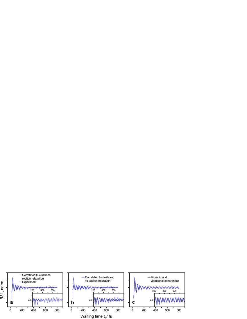
Figure 10: Correlated fluctuation model. a, Simulated beating signal for R31 in the presence of correlated fluctuations (without quasi-resonant vibrations). The modeled curve is shown as a solid blue line and experimental results are shown as a light blue line. Here we take the lowest decoherence rate $\Gamma_{13}\approx(100\,{\rm fs})^{-1}$ of the inter-exciton coherence allowed by correlated fluctuations, constrained by experimentally determined population transfer rates from band 3 to bands 1 and 2. As shown in the inset, correlated fluctuations cannot explain the experimentally measured long-lived beating signal in R31. b, Simulated beating signal for R31 in the absence of the exciton relaxation, shown as a solid blue line. The correlated fluctuation model predicts the lowest decoherence rate $\Gamma_{13}\approx(303\,{\rm fs})^{-1}$ of the inter-exciton coherence when there is no exciton relaxation, even though this condition is not satisfied for C8O3. Nevertheless, the correlated fluctuation model cannot explain the experimentally measured long-lived beating signal in R31, which persist beyond $t_{2}\approx 800\,{\rm fs}$, as shown in an inset. c, Simulated beating signal for R31 in the presence of a vibrational mode with frequency $\hbar\nu_{1}\approx 668\,{\rm cm}^{-1}$, which is quasi-resonant with the exciton energy splitting $\Delta\Omega_{31}$ between bands 1 and 3. Here the vibronic and vibrational coherences induce a long-lived beating signal in good agreement with the experimental results. The root-mean-square deviation (RMSD) of the experimental results and theoretical prediction in a, b and c is 0.74, 0.86 and 0.59, respectively. We note that the correlated fluctuation model can also not explain the long-lasting beating signal in N11 (not shown).

We note that our results are not sensitive to the estimated values of the population transfer rates. The inter-exciton decoherence rate $\Gamma_{13}$ is minimized when there is no population transfer between excitons, i.e. $\gamma_{k\rightarrow l}=0$ for all $k\neq l$, where the coherences between electronic ground state and excitons are destroyed only by pure dephasing noise, i.e. $\hbar\Gamma_{g1}=\hbar\gamma_{g1}\approx 65\,{\rm cm}^{-1}$ and $\hbar\Gamma_{g3}=\hbar\gamma_{g3}\approx 150\,{\rm cm}^{-1}$. Even though this condition is not satisfied for C8O3, this is the best scenario of the correlated fluctuation model where the decoherence rate $\Gamma_{13}$ of the inter-exciton coherence is minimized

$$\Gamma_{13}=\gamma_{13}\geq\left(\sqrt{\gamma_{g1}}-\sqrt{\gamma_{g3}}\,\,\right)^{2}\approx(303\,{\rm fs})^{-1}.$$ (59)

However, even in this case, the lowest decoherence rate $\Gamma_{13}\approx(303\,{\rm fs})^{-1}$ supported by correlated fluctuations is not low enough to explain the experimentally measured long-lived beating signals in N11 and R31, which persist beyond $t_{2}\approx 800\,{\rm fs}$, as shown in Fig. 10b. This is due to the different decoherence rates $\Gamma_{g1}<\Gamma_{g3}$ of $\left|{g}\right\rangle\left\langle{1}\right|$ and $\left|{g}\right\rangle\left\langle{3}\right|$ observed in the experiment. This leads to a non-zero lower bound on the inter-exciton decoherence rate $\Gamma_{13}$, as shown in Eq. (59). In addition, the beating signals in N11 and R31 consist of a short-lived component with 1/e decay time of $\sim$$\,66\,{\rm fs}$ as well as a long-lived component persisting up to $t_{2}\approx 1\,{\rm ps}$. This is contrary to the prediction of the correlated fluctuation model where a single oscillatory component is expected with 1/e decay time of $\Gamma_{13}^{-1}$. For a comparison, the theoretical prediction of the vibronic model is shown in Fig. 10c, where both short-lived and long-lived components are present. We note that in the vibronic model, the decay rate of the long-lived component is independent of $\Gamma_{g1}$ and $\Gamma_{g3}$, as it is determined by the other degrees of freedom, such as the dissipation rate $\gamma_{v}$ of the vibrations and the degree of vibronic mixing $\epsilon_{2}$ leading to a lifetime borrowing effect $\delta\gamma$, as shown in Eq. (30).

We now derive Eqs. (54)-(57) using the Markovian quantum master equation in Eq. (52).

(Dephasing noise) We start with the case that $\omega=0$, leading to the pure dephasing noise. For the sake of simplicity, we assume that there is no degeneracy in the exciton energies $\Omega_{k}$, such that $\Omega_{k}\neq\Omega_{l}$ for all $k\neq l$. In this case, $A_{\alpha}(0)=\sum_{k}\left|{k}\right\rangle\left\langle{k}\right|A_{\alpha}\left|{k}\right\rangle\left\langle{k}\right|=\sum_{k}\left|\left\langle k|e_{\alpha}\right\rangle\right|^{2}\left|{k}\right\rangle\left\langle{k}\right|$. By substituting $\left|{g}\right\rangle\left\langle{1}\right|$, $\left|{g}\right\rangle\left\langle{3}\right|$ and $\left|{1}\right\rangle\left\langle{3}\right|$ to the dissipator of the quantum master equation for $\omega=0$

$$\frac{d}{dt}\rho(t)=\sum_{\alpha,\beta}\gamma_{\alpha\beta}(0)\left(A_{\beta}(0)\rho(t)A_{\alpha}^{\dagger}(0)-\frac{1}{2}\{A_{\alpha}^{\dagger}(0)A_{\beta}(0),\rho(t)\}\right),$$ (60)

one obtains the following pure dephasing rates of the coherences $\left|{g}\right\rangle\left\langle{1}\right|$, $\left|{g}\right\rangle\left\langle{3}\right|$ and $\left|{1}\right\rangle\left\langle{3}\right|$

$$\gamma_{g1} =\frac{1}{2}\sum_{\alpha,\beta}\left|\left\langle 1|e_{\alpha}\right\rangle\right|^{2}\gamma_{\alpha\beta}(0)\mathinner{|\langle 1|e_{\beta}\rangle|}^{2}=\mathinner{|\vec{v}_{1}|}^{2},$$ (61)

$$\gamma_{g3} =\frac{1}{2}\sum_{\alpha,\beta}\left|\left\langle 3|e_{\alpha}\right\rangle\right|^{2}\gamma_{\alpha\beta}(0)\mathinner{|\langle 3|e_{\beta}\rangle|}^{2}=\mathinner{|\vec{v}_{3}|}^{2},$$ (62)

$$\gamma_{13} =\frac{1}{2}\sum_{\alpha,\beta}\left(\left|\left\langle 1|e_{\alpha}\right\rangle\right|^{2}-\left|\left\langle 3|e_{\alpha}\right\rangle\right|^{2}\right)\gamma_{\alpha\beta}(0)\left(\mathinner{|\langle 1|e_{\beta}\rangle|}^{2}-\mathinner{|\langle 3|e_{\beta}\rangle|}^{2}\right)=\mathinner{|\vec{v}_{1}-\vec{v}_{3}|}^{2},$$ (63)

where $\vec{v}_{k}$ represents a vector defined by $\vec{v}_{k}=2^{-1/2}\hat{\gamma}^{1/2}\vec{w}_{k}$: here $\vec{w}_{k}$ is a real vector with elements $\left|\left\langle k|e_{\alpha}\right\rangle\right|^{2}\geq 0$ and $\hat{\gamma}$ is a positive matrixBreuer_SI with elements $\gamma_{\alpha\beta}(0)$, leading to to a positive matrix $\hat{\gamma}^{1/2}$ defined by $\hat{\gamma}=\hat{\gamma}^{1/2}\hat{\gamma}^{1/2}$. For given pure dephasing rates $\gamma_{g1}=\mathinner{|\vec{v}_{1}|}^{2}$ and $\gamma_{g3}=\mathinner{|\vec{v}_{3}|}^{2}$, the inter-exciton pure dephasing rate $\gamma_{13}$ is constrained by

$$\gamma_{13}=\mathinner{|\vec{v}_{1}-\vec{v}_{3}|}^{2}\geq(\mathinner{|\vec{v}_{1}|}-\mathinner{|\vec{v}_{3}|})^{2}=\left(\sqrt{\gamma_{g1}}-\sqrt{\gamma_{g3}}\,\,\right)^{2},$$ (64)

due to the triangle inequality, $\mathinner{|\vec{v}_{1}-\vec{v}_{3}|}+\mathinner{|\vec{v}_{3}|}\geq\mathinner{|\vec{v}_{1}|}$ and $\mathinner{|\vec{v}_{1}-\vec{v}_{3}|}+\mathinner{|\vec{v}_{1}|}\geq\mathinner{|\vec{v}_{3}|}$. Here the equality holds if and only if $\vec{v}_{1}$ is parallel to $\vec{v}_{3}$, which depends on $\hat{\gamma}^{1/2}$ (spectral densities and correlated fluctuations) as well as $\vec{w}_{1}$ and $\vec{w}_{3}$ (the spatial overlap between excitonic wavefunctions). Note that the lower bound in Eq. (64) has been derived based on the positivity of $\hat{\gamma}^{1/2}$, which is satisfied for any spectral densities and correlated fluctuations. These results imply that the inter-exciton dephasing rate $\gamma_{13}$ can be reduced by the correlated fluctuations as well as the spatial overlap between excitonic wavefunctions.

(Exciton relaxation) We now consider the case that $\omega\neq 0$, leading to the incoherent population transfer between excitons. With $\Delta\Omega_{kl}=\Omega_{k}-\Omega_{l}$ denoting the exciton energy splitting between bands $k$ and $l$, $A_{\alpha}(\omega)=\sum_{k,l}\delta(\omega,\Delta\Omega_{kl})\left|{l}\right\rangle\left\langle{l}\right|A_{\alpha}\left|{k}\right\rangle\left\langle{k}\right|=\sum_{k,l}\delta(\omega,\Delta\Omega_{kl})\left\langle l|e_{\alpha}\right\rangle\left\langle e_{\alpha}|k\right\rangle\left|{l}\right\rangle\left\langle{k}\right|$ and the dissipator of the quantum master equation for $\omega\neq 0$ is given by

$$\frac{d}{dt}\rho(t) =\sum_{k\neq l}\sum_{\alpha,\beta}\gamma_{\alpha\beta}(\Delta\Omega_{kl})\left(A_{\beta}(\Delta\Omega_{kl})\rho(t)A_{\alpha}^{\dagger}(\Delta\Omega_{kl})-\frac{1}{2}\{A_{\alpha}^{\dagger}(\Delta\Omega_{kl})A_{\beta}(\Delta\Omega_{kl}),\rho(t)\}\right),$$ (65)

where the population transfer rate $\gamma_{k\rightarrow l}$ from band $k$ to band $l$ is given by

$$\gamma_{k\rightarrow l}=\sum_{\alpha,\beta}\left\langle k|e_{\alpha}\right\rangle\left\langle e_{\alpha}|l\right\rangle\gamma_{\alpha\beta}(\Delta\Omega_{kl})\mathinner{\langle l|e_{\beta}\rangle\langle e_{\beta}|k\rangle}\geq 0,$$ (66)

which is positive, as $\gamma_{\alpha\beta}(\Delta\Omega_{kl})$ form a positive matrixBreuer_SI for given $\Delta\Omega_{kl}$. By substituting $\left|{g}\right\rangle\left\langle{1}\right|$, $\left|{g}\right\rangle\left\langle{3}\right|$ and $\left|{1}\right\rangle\left\langle{3}\right|$ to the dissipators in Eqs. (60) and (65), one can show that the electronic decoherence rates $\Gamma_{g1}$, $\Gamma_{g3}$ and $\Gamma_{13}$ satisfy Eqs. (54)-(57). These results are valid for any spectral densities and correlated fluctuations within the level of the Markovian quantum master equation in Eq. (52), which includes the theoretical models considered in previous studiesRebentrost_JPCB2009_SI .

In summary, the correlated fluctuation model cannot explain the long-lived beating signals in N11 and R31 within the level of Markovian quantum master equations, as the decoherence rate $\Gamma_{13}$ of the inter-exciton coherence $\left|{1}\right\rangle\left\langle{3}\right|$ is constrained by the experimentally observed asymmetric decoherence rates $\Gamma_{g1}$ and $\Gamma_{g3}$, i.e. $\Gamma_{g3}\approx 2\Gamma_{g1}$, and the fast population transfer from band 3 to bands 1 and 2. We note that the asymmetric decoherence rates $\Gamma_{g1}$ and $\Gamma_{g3}$ are related to the fact that i) the lineshape of R31 is elongated along $\omega_{1}$-axis (cf. Figures 2b and d in the main text), ii) the amplitudes of the short-lived beating signals in N11 and R31 are different in magnitude (cf. Figures 3b and c in the main text), and iii) the absorptive linewidths of bands 1 and 3 are different (cf. Fig. 6 in the SI).

III References

References

(1) Van Amerongen, H., Valkunas, L. & Van Grondelle, R. Photosynthetic
excitons (World Scientific, Singapore, 2000).
(2) Blankenship, R. E. Molecular mechanisms of photosynthesis (Blackwell Science, Oxford, 2002).
(3) Renger, T., May, V. & Kühn, O. Ultrafast excitation energy transfer
dynamics in photosynthetic pigment-protein complexes. Physics
Reports343, 137–254 (2001).
(4) Huelga, S. F. & Plenio, M. B. Vibrations, quanta and biology. Contemp. Phys.54, 181–207 (2013).
(5) Jonas, D. M. Two-dimensional femtosecond spectroscopy. Annu. Rev.
Phys. Chem.54, 425–463 (2003).
(6) Engel, G. S. et al. Evidence for
wavelike energy transfer through quantum coherence in photosynthetic
systems. Nature446, 782–786 (2007).
(7) Dostál, J., Mančal, T., Vácha, F., Pšenčík, J. &
Zigmantas, D. Unraveling the nature of coherent beatings in
chlorosomes. J. Chem. Phys.140, 115103 (2014).
(8)
Collini, E. et al. Coherently wired light-harvesting in photosynthetic
marine algae at ambient temperature. Nature463, 644–647
(2010).
(9)
Romero, E. et al. Quantum coherence in
photosynthesis for efficient solar-energy conversion. Nature Phys.10, 676–682 (2014).
(10)
Fuller, F. D. et al. Vibronic coherence in oxygenic photosynthesis. Nature
Chem.6, 706–711 (2014).
(11)
Chin, A. W. et al. The role of non-equilibrium vibrational structures in
electronic coherence and recoherence in pigment-protein complexes. Nature Phys.9, 113–118 (2013).
(12)
Plenio, M. B., Almeida, J. & Huelga, S. F. Origin of long-lived
oscillations in 2D-spectra of a quantum vibronic model: electronic versus
vibrational coherence. J. Chem. Phys.139, 235102 (2013).
(13)
Chin, A. W., Huelga, S. F. & Plenio, M. B. Coherence and decoherence
in biological system: principles of noise assisted transport and the origin
of long-lived coherences. Phil. Trans. Act. Roy. Soc. A370,
3638–3657 (2012).
(14)
Kolli, A., O’Reilly, E. J., Scholes, G. D. & Olaya-Castro, A. The
fundamental role of quantized vibrations in coherent light harvesting by
cryptophyte algae. J. Chem. Phys.137, 174109 (2012).
(15)
Tiwari, V., Peters, W. K. & Jonas, D. M. Electronic resonance with
anticorrelated pigment vibrations drives photosynthetic energy transfer
outside the adiabatic framework. PNAS110, 1203–1208
(2013).
(16)
Lee, H., Cheng, Y.-C. & Fleming, G. R. Coherence dynamics in
photosynthesis: protein protection of excitonic coherence. Science316, 1462–1465 (2007).
(17)
Ishizaki, A., Calhoun, T. R., Schlau-Cohen, G. S. & Fleming, G. R.
Quantum coherence and its interplay with protein environments in
photosynthetic electronic energy transfer. Phys. Chem. Chem. Phys.12, 7319–7337 (2010).
(18)
Hayes, D., Griffin, G. B. & Engel, G. S. Engineering coherence among
excited states in synthetic heterodimer systems. Science340,
1431–1434 (2013).
(19)
Christensson, N. et al. High frequency vibrational modulations
in two-dimensional electronic spectra and their resemblance to electronic
coherence signatures. J. Phys. Chem. B115, 5383–5391
(2011).
(20)
Caycedo-Soler, F., Chin, A. W., Almeida, J., Huelga, S. F. &
Plenio, M. B. The nature of the low energy band of the Fenna-Matthews-Olson
complex: vibronic signatures. J. Chem. Phys.136, 155102
(2012).
(21)
Christensson, N., Kauffmann, H. F., Pullerits, T. & Mančal, T.
Origin of long-lived coherences in light-harvesting complexes. J.
Phys. Chem. B116, 7449–7454 (2012).
(22)
Heijs, D.-J., Dijkstra, A. G. & Knoester, J. Ultrafast pump-probe
spectroscopy of linear molecular aggregates: effects of exciton coherence and
thermal dephasing. Chem. Phys.341, 230–239 (2007).
(23)
Würthner, F., Kaiser, T. E. & Saha-Möller, C. R.
J-aggregates: from serendipitous discovery to supramolecular engineering
of functional dye materials. Angew. Chem. Int. Ed.50,
3376–3410 (2011).
(24)
Eisele, D. M. et al. Robust
excitons inhabit soft supramolecular nanotubes. PNAS111,
E3367–E3375 (2014).
(25)
Yuen-Zhou, J. et al. Coherent exciton
dynamics in supramolecular light-harvesting nanotubes revealed by ultrafast
quantum process tomography. ACS Nano8, 5527–5534 (2014).
(26)
Qiao, Y. et al. Nanotubular J-aggregates and quantum dots
coupled for efficient resonance excitation energy transfer. ACS
Nano9, 1552–1560 (2015).
(27)
Von Berlepsch, H. & Böttcher, C. The morphologies of molecular
cyanine dye aggregates as revealed by cryogenic transmission electron
microscopy (World Scientific, Singapore, 2012).
(28)
Von Berlepsch, H., Kirstein, S. & Böttcher, C. Effect of alcohols on
J-aggregation of a carbocyanine dye. Langmuir18,
7699–7705 (2002).
(29)
Von Berlepsch, H., Kirstein, S. & Böttcher, C. Controlling the helicity
of tubular J-aggregates by chiral alcohols. J. Phys. Chem. B107, 9646–9654 (2003).
(30)
Von Berlepsch, H. et al. Supramolecular structures of J-aggregates of
carbocyanine dyes in solution. J. Phys. Chem. B104,
5255–5262 (2000).
(31)
Von Berlepsch, H. et al. Stabilization of individual tubular J-aggregates
by poly(vinyl alcohol). J. Phys. Chem. B107,
14176–14184 (2003).
(32)
Eisele, D. M. et al. Utilizing redox-chemistry to elucidate the nature of exciton
transitions in supramolecular dye nanotubes. Nature Chem.4,
655–662 (2012).
(33)
Milota, F. et al. Vibronic and vibrational
coherences in two-dimensional electronic spectra of supramolecular
J-aggregates. J. Phys. Chem. A117, 6007–6014 (2013).
(34)
Aydin, M., Dede, Ö. & Akins, D. L. Density functional theory and
Raman spectroscopy applied to structure and vibrational mode analysis of
1,1’,3,3’-tetraethyl-5,5’,6,6’-tetrachloro-benzimidazolocarbocyanine iodide
and its aggregate. J. Chem. Phys.134, 064325 (2011).
(35)
Rich, C. C. & McHale, J. L. Resonance Raman spectra of individual
excitonically coupled chromophore aggregates. J. Phys. Chem. C117, 10856–10865 (2013).
(36)
Butkus, V., Zigmantas, D., Abramavicius, D. & Valkunas, L. Distinctive
character of electronic and vibrational coherences in disordered molecular
aggregates. Chem. Phys. Lett.587, 93–98 (2013).
(37)
Womick, J. M. & Moran, A. M. Exciton coherence and energy transport in
the light-harvesting dimers of allophycocyanin. J. Phys. Chem. B113, 15747–15759 (2009).
(38)
Womick, J. M. & Moran, A. M. Vibronic enhancement of exciton sizes and
energy transport in photosynthetic complexes. J. Phys. Chem. B115, 1347–1356 (2011).
(39)
Del Rey, M., Chin, A. W., Huelga, S. F. & Plenio, M. B. Exploiting
structured environments for efficient energy transfer: the phonon antenna
mechanism. J. Phys. Chem. Lett.4, 903–907 (2013).
(40)
Hochstrasser, R. M. Two-dimensional IR-spectroscopy: polarization
anisotropy effects. Chem. Phys.266, 273–284 (2001).
(41)
Read, E. L. et al. Cross-peak-specific
two-dimensional electronic spectroscopy. PNAS104,
14203–14208 (2007).
(42)
Mukamel, S. Principles of nonlinear optical spectroscopy (Oxford University Press, Oxford, 1995).
(43)
Perlík, V. et al. Vibronic coupling explains the ultrafast carotenoid-to-bacteriochlorophyll energy transfer in natural and artificial light harvesters. J. Chem. Phys.142, 212434 (2015).
(44)
Schröter, M. et al. Exciton-vibrational coupling in the dynamics and spectroscopy of Frenkel excitons in molecular aggregates. Phys. Rep.567, 1–78 (2015).
(45)
Killoran, N., Huelga, S. F. & Plenio, M. B. Enhancing
light-harvesting power with coherent vibrational interactions: a quantum heat
engine picture. Preprint at http://arxiv.org/abs/1412.4136 (2015).
(46)
Didraga, C. et al. Structure, spectroscopy, and microscopic model of
tubular carbocyanine dye aggregates. J. Phys. Chem. B108,
14976–14985 (2004).
(47)
Halpin, A. et al. Two-dimensional spectroscopy of
a molecular dimer unveils the effects of vibronic coupling on exciton
coherences. Nature Chem.6, 196–201 (2014).
(48)
Chenu, A. & Scholes, G. D. Coherence in energy transfer and photosynthesis. Annu. Rev. Phys. Chem.66, 69–96 (2015).
(49)
Falke, S. M. et al. Coherent ultrafast
charge transfer in an organic photovoltaic blend. Science344,
1001–1005 (2014).
(50)
Brixner, T., Mančal, T., Stiopkin, I. V. & Fleming, G. R.
Phase-stabilized two-dimensional electronic spectroscopy. J. Chem.
Phys.121, 4221–4236 (2004).
(51)
Augulis, R. & Zigmantas, D. Two-dimensional electronic spectroscopy
with double modulation lock-in detection: enhancement of sensitivity and
noise resistance. Opt. Express19, 13126–13133 (2011).
(52)
Augulis, R. & Zigmantas, D. Detector and dispersive delay calibration
issues in broadband 2D electronic spectroscopy. J. Opt. Soc. Am. B30, 1770–1774 (2013).

References

(1)
Dékány, Gy., Csóka, I. & Erös, I. Adsorption of
neutral polymers on negatively charged liposomes. A novel quantitative method
to measure the rate of polymer adsorption on the liposomal surface. Colloid Polym. Sci.279, 966–975 (2001).
(2)
Eisele, D. M. et al. Robust
excitons inhabit soft supramolecular nanotubes. PNAS111,
E3367–E3375 (2014).
(3)
Von Berlepsch, H. et al. Stabilization of individual tubular J-aggregates
by poly(vinyl alcohol). J. Phys. Chem. B107,
14176–14184 (2003).
(4)
Tauber, M. J., Mathies, R. A., Chen, X. & Bradforth, S. E. Flowing
liquid sample jet for resonance Raman and ultrafast optical spectroscopy.
Rev. Sci. Instrum.74, 4958–4960 (2003).
(5)
Brixner, T., Mančal, T., Stiopkin, I. V. & Fleming, G. R.
Phase-stabilized two-dimensional electronic spectroscopy. J. Chem.
Phys.121, 4221–4236 (2004).
(6)
Augulis, R. & Zigmantas, D. Two-dimensional electronic spectroscopy
with double modulation lock-in detection: enhancement of sensitivity and
noise resistance. Opt. Express19, 13126–13133 (2011).
(7)
Hochstrasser, R. M. Two-dimensional IR-spectroscopy: polarization
anisotropy effects. Chem. Phys.266, 273–284 (2001).
(8)
Schlau-Cohen, G. S. et al. Elucidation of the
timescales and origins of quantum electronic coherence in LHCII. Nature Chem.4, 389–395 (2012).
(9)
Westenhoff, S. Paleček, D., Edlund, P., Smith, P. & Zigmantas, D.
Coherent picosecond exciton dynamics in a photosynthetic reaction
center. J. Am. Chem. Soc.134, 16484–16487 (2012).
(10)
Jonas, D. M. Two-dimensional femtosecond spectroscopy. Annu. Rev.
Phys. Chem.54, 425–463 (2003).
(11)
Milota, F., Lincoln, C. N. & Hauer, J. Precise phasing of
2D-electronic spectra in a fully non-collinear phase-matching geometry.
Opt. Express21, 15904–15911 (2013).
(12)
Breuer, H. & Petruccione, F. The theory of open quantum systems(Oxford University Press, 2002).
(13)
Didraga, C. et al. Structure, spectroscopy, and microscopic model of
tubular carbocyanine dye aggregates. J. Phys. Chem. B108,
14976–14985 (2004).
(14)
Tiwari, V., Peters, W. K. & Jonas, D. M. Electronic resonance with
anticorrelated pigment vibrations drives photosynthetic energy transfer
outside the adiabatic framework. PNAS110, 1203–1208
(2013).
(15)
Lidar, D. A., Chuang, I. L. & Whaley, K. B. Decoherence-free
subspaces for quantum computation. Phys. Rev. Lett.81,
2594 (1998).
(16)
Rebentrost, P., Mohseni, M. & Aspuru-Guzik, A. Role of quantum
coherence and environmental fluctuations in chromophoric energy transport.
J. Phys. Chem. B113, 9942–9947 (2009).
(17)
Milota, F. et al. Vibronic and vibrational
coherences in two-dimensional electronic spectra of supramolecular
J-aggregates. J. Phys. Chem. A117, 6007–6014 (2013).