A q๐‘žq-enumeration of lozenge tilings of a hexagon with four adjacent triangles removed from the boundary

Tri Lai Department of Mathematics
University of Nebraskaโ€“Lincoln, Lincoln, NE 68588
Abstract

MacMahon proved a simple product formula for the generating function of plane partitions fitting in a given box. The theorem implies a q๐‘žq-enumeration of lozenge tilings of a semi-regular hexagon on the triangular lattice. In this paper we generalize MacMahonโ€™s classical theorem by q๐‘žq-enumerating lozenge tilings of a new family of hexagons with four adjacent triangles removed from their boundary.

keywords:
Graphical condensation , Lozenge tilings , Perfect matchings , Plane partitions
MSC:
[2010] 05A15 , 05C30 , 05C70

1 Introduction and main results

Given k๐‘˜k positive integers ฮป1โ‰ฅฮป2โ‰ฅโ‹ฏโ‰ฅฮปksubscript๐œ†1subscript๐œ†2โ‹ฏsubscript๐œ†๐‘˜\lambda_{1}\geq\lambda_{2}\geq\dots\geq\lambda_{k}, a plane partition of shape (ฮป1,ฮป2,โ€ฆ,ฮปk)subscript๐œ†1subscript๐œ†2โ€ฆsubscript๐œ†๐‘˜(\lambda_{1},\lambda_{2},\dots,\lambda_{k}) is an array of non-negative integers

n1,1subscript๐‘›11n_{1,1} n1,2subscript๐‘›12n_{1,2} n1,3subscript๐‘›13n_{1,3} โ€ฆโ€ฆ\dotsc โ€ฆโ€ฆ\dotsc โ€ฆโ€ฆ\dotsc n1,ฮป1subscript๐‘›1subscript๐œ†1n_{1,\lambda_{1}}
n2,1subscript๐‘›21n_{2,1} n2,2subscript๐‘›22n_{2,2} n2,3subscript๐‘›23n_{2,3} โ€ฆโ€ฆ\dotsc โ€ฆโ€ฆ\dotsc n2,ฮป2subscript๐‘›2subscript๐œ†2n_{2,\lambda_{2}}
โ‹ฎโ‹ฎ\vdots โ‹ฎโ‹ฎ\vdots โ‹ฎโ‹ฎ\vdots โ‹ฎโ‹ฎ\vdots

โ‹ฑโ‹ฑ\ddots

nk,1subscript๐‘›๐‘˜1n_{k,1} nk,2subscript๐‘›๐‘˜2n_{k,2} nk,3subscript๐‘›๐‘˜3n_{k,3} โ€ฆโ€ฆ\dotsc nk,ฮปksubscript๐‘›๐‘˜subscript๐œ†๐‘˜n_{k,\lambda_{k}}

so that ni,jโ‰ฅni,j+1subscript๐‘›๐‘–๐‘—subscript๐‘›๐‘–๐‘—1n_{i,j}\geq n_{i,j+1} and ni,jโ‰ฅni+1,jsubscript๐‘›๐‘–๐‘—subscript๐‘›๐‘–1๐‘—n_{i,j}\geq n_{i+1,j} (i.e. all rows and all columns are weakly decreasing from left to right and from top to bottom, respectively). The sum of all entries of a plane partition ฯ€๐œ‹\pi is called the volume (or the norm) of the plane partition, and denoted by |ฯ€|๐œ‹|\pi|.

The plane partitions of rectangular shape (b,b,โ€ฆ,b)๐‘๐‘โ€ฆ๐‘(b,b,\dots,b) (a๐‘Ža rows) with entries at most c๐‘c are usually identified with their 3-D interpretations โ€” piles (or stacks) of unit cubes fitting in an aร—bร—c๐‘Ž๐‘๐‘a\times b\times c box. The latter are in bijection with lozenge tilings of a semi-regular hexagon Hโ€‹eโ€‹xโ€‹(a,b,c)๐ป๐‘’๐‘ฅ๐‘Ž๐‘๐‘Hex(a,b,c) of side-lengths a,b,c,a,b,c๐‘Ž๐‘๐‘๐‘Ž๐‘๐‘a,b,c,a,b,c (in clockwise order, starting from the northwest side111From now on, we always list the side-lengths of a hexagon on the triangular lattice in the clockwise order, starting from the northwest side.) on the triangular lattice. Here, a lozenge (or unit rhombus) is union of any two unit equilateral triangles sharing an edge; and a lozenge tiling of a region is a covering of the region by lozenges so that there are no gaps or overlaps.

Let q๐‘žq be an indeterminate. The q๐‘žq-integer [n]qsubscriptdelimited-[]๐‘›๐‘ž[n]_{q} is defined by [n]q:=1+q+q2+โ€ฆ+qnโˆ’1assignsubscriptdelimited-[]๐‘›๐‘ž1๐‘žsuperscript๐‘ž2โ€ฆsuperscript๐‘ž๐‘›1[n]_{q}:=1+q+q^{2}+\dotsc+q^{n-1}. We also define the q๐‘žq-factorial by [n]q!:=[1]qโ‹…[2]qโ€‹โ€ฆโ€‹[n]qassignsubscriptdelimited-[]๐‘›๐‘žโ‹…subscriptdelimited-[]1๐‘žsubscriptdelimited-[]2๐‘žโ€ฆsubscriptdelimited-[]๐‘›๐‘ž[n]_{q}!:=[1]_{q}\cdot[2]_{q}\dotsc[n]_{q}, and the q๐‘žq-hyperfactorial function by Hqโก(n):=[0]q!โ‹…[1]q!โ‹…[2]q!โ€‹โ€ฆโ€‹[nโˆ’1]q!assignsubscriptH๐‘ž๐‘›โ‹…subscriptdelimited-[]0๐‘žsubscriptdelimited-[]1๐‘žsubscriptdelimited-[]2๐‘žโ€ฆsubscriptdelimited-[]๐‘›1๐‘ž\operatorname{H}_{q}(n):=[0]_{q}!\cdot[1]_{q}!\cdot[2]_{q}!\dotsc[n-1]_{q}!. MacMahon [29] proved that the volume generating function of the plane partitions fitting in an aร—bร—c๐‘Ž๐‘๐‘a\times b\times c box is given by

โˆ‘ฯ€q|ฯ€|=Hqโก(a)โ€‹Hqโก(b)โ€‹Hqโก(c)โ€‹Hqโก(a+b+c)Hqโก(a+b)โ€‹Hqโก(b+c)โ€‹Hqโก(c+a),subscript๐œ‹superscript๐‘ž๐œ‹subscriptH๐‘ž๐‘ŽsubscriptH๐‘ž๐‘subscriptH๐‘ž๐‘subscriptH๐‘ž๐‘Ž๐‘๐‘subscriptH๐‘ž๐‘Ž๐‘subscriptH๐‘ž๐‘๐‘subscriptH๐‘ž๐‘๐‘Ž\sum_{\pi}q^{|\pi|}=\frac{\operatorname{H}_{q}(a)\operatorname{H}_{q}(b)\operatorname{H}_{q}(c)\operatorname{H}_{q}(a+b+c)}{\operatorname{H}_{q}(a+b)\operatorname{H}_{q}(b+c)\operatorname{H}_{q}(c+a)}, (1.1)

where the sum on the left-hand side is taken over all plane partitions ฯ€๐œ‹\pi fitting in an aร—bร—c๐‘Ž๐‘๐‘a\times b\times c box. By specializing q=1๐‘ž1q=1 in the MacMahon formula (1.1), it follows that the number of lozenge tilings of a semi-regular hexagon Hโ€‹eโ€‹xโ€‹(a,b,c)๐ป๐‘’๐‘ฅ๐‘Ž๐‘๐‘Hex(a,b,c) is equal to

Hโก(a)โ€‹Hโก(b)โ€‹Hโก(c)โ€‹Hโก(a+b+c)Hโก(a+b)โ€‹Hโก(b+c)โ€‹Hโก(c+a),H๐‘ŽH๐‘H๐‘H๐‘Ž๐‘๐‘H๐‘Ž๐‘H๐‘๐‘H๐‘๐‘Ž\frac{\operatorname{H}(a)\operatorname{H}(b)\operatorname{H}(c)\operatorname{H}(a+b+c)}{\operatorname{H}(a+b)\operatorname{H}(b+c)\operatorname{H}(c+a)}, (1.2)

where Hโก(n):=H1โก(n)=0!โ‹…1!โ‹…2!โ€‹โ€ฆโ€‹(nโˆ’1)!assignH๐‘›subscriptH1๐‘›โ‹…012โ€ฆ๐‘›1\operatorname{H}(n):=\operatorname{H}_{1}(n)=0!\cdot 1!\cdot 2!\dotsc(n-1)! is the ordinary hyperfactorial function.

The tiling formula (1.2) inspired a large body of work focusing on enumeration of lozenge tilings of a hexagon with dents or holes (see e.g. [3], [7], [5], [8], [15], [16], [13], [14], [18], [25], [33]). Here, a dent is a portion of the hexagon that has been removed from the boundary, while a hole is a portion removed from inside the hexagon.

Refer to caption
Figure 1.1: The shamrock S4,2,2,3subscript๐‘†4223S_{4,2,2,3}.

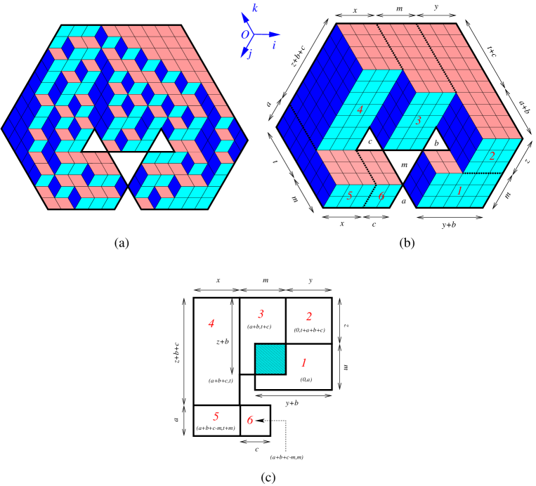
In this paper, we consider a new type of dented hexagon as follows. The shamrock222The shamrock was first introduced by Ciucu and Krattenthaler in [8]. Sm,a,b,csubscript๐‘†๐‘š๐‘Ž๐‘๐‘S_{m,a,b,c} is the union of four equilateral triangles with sides m๐‘šm, a๐‘Ža, b๐‘b, c๐‘c on the triangular lattice described in Figure 1.1. We start with a hexagon of side-lengths z+a+b+c,x+y+m,t+a+b+c,z+m,x+y+a+b+c,t+m๐‘ง๐‘Ž๐‘๐‘๐‘ฅ๐‘ฆ๐‘š๐‘ก๐‘Ž๐‘๐‘๐‘ง๐‘š๐‘ฅ๐‘ฆ๐‘Ž๐‘๐‘๐‘ก๐‘šz+a+b+c,x+y+m,t+a+b+c,z+m,x+y+a+b+c,t+m, where x,y,z,t๐‘ฅ๐‘ฆ๐‘ง๐‘กx,y,z,t are four non-negative integers. Next, we remove a shamrock Sm,a,b,csubscript๐‘†๐‘š๐‘Ž๐‘๐‘S_{m,a,b,c} from the base of the hexagon so that the lower-left vertex of the a๐‘Ža-triangle in the shamrock is x+c๐‘ฅ๐‘x+c units to the right of the lower-left vertex of the hexagon. We denote by Qโ€‹(xyztmabc)๐‘„matrix๐‘ฅ๐‘ฆ๐‘ง๐‘ก๐‘š๐‘Ž๐‘๐‘Q\begin{pmatrix}x&y&z&t\\ m&a&b&c\end{pmatrix} the resulting region. Figure 1.2 shows the region Qโ€‹(43234321)๐‘„matrix43234321Q\begin{pmatrix}4&3&2&3\\ 4&3&2&1\end{pmatrix}.

Refer to caption
Figure 1.2: Hexagon with a shamrock removed along the boundary.

Our following main theorem shows that the lozenge tilings of a Q๐‘„Q-type region are always enumerated by a simple product formula.

Theorem 1.1.

For non-negative integers x,y,z,t,m,a,b,c๐‘ฅ๐‘ฆ๐‘ง๐‘ก๐‘š๐‘Ž๐‘๐‘x,y,z,t,m,a,b,c, the number of lozenge tilings of the region Qโ€‹(xyztmabc)๐‘„matrix๐‘ฅ๐‘ฆ๐‘ง๐‘ก๐‘š๐‘Ž๐‘๐‘Q\begin{pmatrix}x&y&z&t\\ m&a&b&c\end{pmatrix} is equal to

Hโก(m+a+b+c+x+y+z+t)Hโก(m+a+b+c+x+y+t)โ€‹Hโก(m+a+b+c+x+y+z)H๐‘š๐‘Ž๐‘๐‘๐‘ฅ๐‘ฆ๐‘ง๐‘กH๐‘š๐‘Ž๐‘๐‘๐‘ฅ๐‘ฆ๐‘กH๐‘š๐‘Ž๐‘๐‘๐‘ฅ๐‘ฆ๐‘ง\displaystyle\frac{\operatorname{H}(m+a+b+c+x+y+z+t)}{\operatorname{H}(m+a+b+c+x+y+t)\operatorname{H}(m+a+b+c+x+y+z)}
ร—Hโก(m+a+b+c+x+t)โ€‹Hโก(m+a+b+c+x+y)โ€‹Hโก(m+a+b+c+y+z)Hโก(m+a+b+c+z+t)โ€‹Hโก(m+a+b+c+x)โ€‹Hโก(m+a+b+c+y)absentH๐‘š๐‘Ž๐‘๐‘๐‘ฅ๐‘กH๐‘š๐‘Ž๐‘๐‘๐‘ฅ๐‘ฆH๐‘š๐‘Ž๐‘๐‘๐‘ฆ๐‘งH๐‘š๐‘Ž๐‘๐‘๐‘ง๐‘กH๐‘š๐‘Ž๐‘๐‘๐‘ฅH๐‘š๐‘Ž๐‘๐‘๐‘ฆ\displaystyle\times\frac{\operatorname{H}(m+a+b+c+x+t)\operatorname{H}(m+a+b+c+x+y)\operatorname{H}(m+a+b+c+y+z)}{\operatorname{H}(m+a+b+c+z+t)\operatorname{H}(m+a+b+c+x)\operatorname{H}(m+a+b+c+y)}
ร—Hโก(x)โ€‹Hโก(y)โ€‹Hโก(z)โ€‹Hโก(t)Hโก(x+t)โ€‹Hโก(y+z)โ€‹H(m)3H(a)2H(b)H(c)H(m+a+b+c)H(m+a)2H(m+b)H(m+c)\displaystyle\times\frac{\operatorname{H}(x)\operatorname{H}(y)\operatorname{H}(z)\operatorname{H}(t)}{\operatorname{H}(x+t)\operatorname{H}(y+z)}\frac{\operatorname{H}(m)^{3}\operatorname{H}(a)^{2}\operatorname{H}(b)\operatorname{H}(c)\operatorname{H}(m+a+b+c)}{\operatorname{H}(m+a)^{2}\operatorname{H}(m+b)\operatorname{H}(m+c)}
ร—Hโก(m+b+c+z+t)โ€‹Hโก(m+a+c+x)โ€‹Hโก(m+a+b+y)Hโก(m+b+y+z)โ€‹Hโก(m+c+x+t)absentH๐‘š๐‘๐‘๐‘ง๐‘กH๐‘š๐‘Ž๐‘๐‘ฅH๐‘š๐‘Ž๐‘๐‘ฆH๐‘š๐‘๐‘ฆ๐‘งH๐‘š๐‘๐‘ฅ๐‘ก\displaystyle\times\frac{\operatorname{H}(m+b+c+z+t)\operatorname{H}(m+a+c+x)\operatorname{H}(m+a+b+y)}{\operatorname{H}(m+b+y+z)\operatorname{H}(m+c+x+t)}
ร—Hโก(c+x+t)โ€‹Hโก(b+y+z)Hโก(a+c+x)โ€‹Hโก(a+b+y)โ€‹Hโก(b+c+z+t).absentH๐‘๐‘ฅ๐‘กH๐‘๐‘ฆ๐‘งH๐‘Ž๐‘๐‘ฅH๐‘Ž๐‘๐‘ฆH๐‘๐‘๐‘ง๐‘ก\displaystyle\times\frac{\operatorname{H}(c+x+t)\operatorname{H}(b+y+z)}{\operatorname{H}(a+c+x)\operatorname{H}(a+b+y)\operatorname{H}(b+c+z+t)}. (1.3)

One readily sees that, by letting a=b=c=m=0๐‘Ž๐‘๐‘๐‘š0a=b=c=m=0, our Q๐‘„Q-type region becomes a semi-regular hexagon. In this sense, Theorem 1.1 is a generalization of MacMahonโ€™s tiling formula (1.2).

If we assign to each lozenge tiling T๐‘‡T of a semi-regular hexagon Hโ€‹eโ€‹xโ€‹(a,b,c)๐ป๐‘’๐‘ฅ๐‘Ž๐‘๐‘Hex(a,b,c) a weight q|ฯ€|superscript๐‘ž๐œ‹q^{|\pi|}, where ฯ€๐œ‹\pi is the plane partition corresponding to T๐‘‡T, the generating function on the left-hand side of (1.1) becomes a weighted sum of the lozenge tilings of Hโ€‹eโ€‹xโ€‹(a,b,c)๐ป๐‘’๐‘ฅ๐‘Ž๐‘๐‘Hex(a,b,c). In this sense, MacMahonโ€™s formula yields a weighted enumeration of lozenge tilings of a semi-regular hexagon. This weighted enumeration is usually called a q๐‘žq-enumeration, since the tiling weights here are all powers of q๐‘žq. While there are many known tiling enumerations of hexagons with dents or holes, most of them only concern โ€˜plain tilingsโ€™ (i.e. tilings without weight). Only a few weighted enumerations have been found (see e.g. [29], [36], [37, pp.374โ€“375], [25]). In the next part of this section, we consider such a rare weighted enumeration, that is a q๐‘žq-analog of the result in Theorem 1.1 (see Theorem 1.2).

Similar to the bijection between lozenge tilings of a semi-regular hexagon Hโ€‹eโ€‹xโ€‹(a,b,c)๐ป๐‘’๐‘ฅ๐‘Ž๐‘๐‘Hex(a,b,c) and plane partitions fitting in an aร—bร—c๐‘Ž๐‘๐‘a\times b\times c box, one can view a lozenge tiling of Qโ€‹(xyztmabc)๐‘„matrix๐‘ฅ๐‘ฆ๐‘ง๐‘ก๐‘š๐‘Ž๐‘๐‘Q\begin{pmatrix}x&y&z&t\\ m&a&b&c\end{pmatrix} as a pile of unit cubes fitting in a compound box โ„ฌ:=โ„ฌโ€‹(xyztmabc)assignโ„ฌโ„ฌmatrix๐‘ฅ๐‘ฆ๐‘ง๐‘ก๐‘š๐‘Ž๐‘๐‘\mathcal{B}:=\mathcal{B}\begin{pmatrix}x&y&z&t\\ m&a&b&c\end{pmatrix}, which is the union of 6 adjacent rectangular boxes (see Figure 1.3(a) for the case when x=y=z=3,t=4,m=3,a=b=c=2formulae-sequence๐‘ฅ๐‘ฆ๐‘ง3formulae-sequence๐‘ก4formulae-sequence๐‘š3๐‘Ž๐‘๐‘2x=y=z=3,t=4,m=3,a=b=c=2). Figure 1.3(b) gives a 3-D picture of the compound box โ„ฌโ„ฌ\mathcal{B} by showing the empty pile; the bases of the rectangular boxes in โ„ฌโ„ฌ\mathcal{B} consist of right-tilted lozenges and are labeled by 1,2,โ€ฆ,612โ€ฆ61,2,\dotsc,6.

Refer to caption
Figure 1.3: (a) Viewing a lozenge tiling of a Q๐‘„Q-type region as a pile of unit cubes fitting in a special box. (b) The tiling corresponding to the empty pile. (c) The projection of the compound box โ„ฌโ„ฌ\mathcal{B} on the Oij plane.

Projecting the compound box โ„ฌโ„ฌ\mathcal{B} on the Oij plane, we get a projective diagram as in Figure 1.3(c). In this diagram, each rectangular box in โ„ฌโ„ฌ\mathcal{B} is represented by a rectangle with a pair of integers (a,b)๐‘Ž๐‘(a,b), where a๐‘Ža is the level of the base and b๐‘b is the height of the box. We always assume that the base of the box 111 is on level 00. We also note that the rectangles corresponding to the boxes 1 and 3 are overlapping (the intersection is indicated by the shaded area in Figure 1.3(c)). However, these two boxes themselves are not overlapping, since the box 333 is hanging over the box 1.

We call the piles of unit cubes fitting in the compound box โ„ฌโ„ฌ\mathcal{B} generalized plane partitions, since they have a similar monotonicity as (the 3D-interpretation of) the ordinary plane partitions: the tops of their columns (of unit cubes) are weakly decreasing along Oiโ†’โ†’Oi\overrightarrow{\textbf{Oi}} and Ojโ†’โ†’Oj\overrightarrow{\textbf{Oj}}.

Similar to MacMahonโ€™s theorem (1.1), we have a closed form product formula for the volume generating function of the generalized plane partitions.

Theorem 1.2.

Let m,a,b,c,x,y,z,t๐‘š๐‘Ž๐‘๐‘๐‘ฅ๐‘ฆ๐‘ง๐‘กm,a,b,c,x,y,z,t be non-negative integers. Then

โˆ‘ฯ€q|ฯ€|subscript๐œ‹superscript๐‘ž๐œ‹\displaystyle\sum_{\pi}q^{|\pi|} =Hqโก(m+a+b+c+x+y+z+t)Hqโก(m+a+b+c+x+y+t)โ€‹Hqโก(m+a+b+c+x+y+z)absentsubscriptH๐‘ž๐‘š๐‘Ž๐‘๐‘๐‘ฅ๐‘ฆ๐‘ง๐‘กsubscriptH๐‘ž๐‘š๐‘Ž๐‘๐‘๐‘ฅ๐‘ฆ๐‘กsubscriptH๐‘ž๐‘š๐‘Ž๐‘๐‘๐‘ฅ๐‘ฆ๐‘ง\displaystyle=\frac{\operatorname{H}_{q}(m+a+b+c+x+y+z+t)}{\operatorname{H}_{q}(m+a+b+c+x+y+t)\operatorname{H}_{q}(m+a+b+c+x+y+z)}
ร—Hqโก(m+a+b+c+x+t)โ€‹Hqโก(m+a+b+c+x+y)โ€‹Hqโก(m+a+b+c+y+z)Hqโก(m+a+b+c+z+t)โ€‹Hqโก(m+a+b+c+x)โ€‹Hqโก(m+a+b+c+y)absentsubscriptH๐‘ž๐‘š๐‘Ž๐‘๐‘๐‘ฅ๐‘กsubscriptH๐‘ž๐‘š๐‘Ž๐‘๐‘๐‘ฅ๐‘ฆsubscriptH๐‘ž๐‘š๐‘Ž๐‘๐‘๐‘ฆ๐‘งsubscriptH๐‘ž๐‘š๐‘Ž๐‘๐‘๐‘ง๐‘กsubscriptH๐‘ž๐‘š๐‘Ž๐‘๐‘๐‘ฅsubscriptH๐‘ž๐‘š๐‘Ž๐‘๐‘๐‘ฆ\displaystyle\times\frac{\operatorname{H}_{q}(m+a+b+c+x+t)\operatorname{H}_{q}(m+a+b+c+x+y)\operatorname{H}_{q}(m+a+b+c+y+z)}{\operatorname{H}_{q}(m+a+b+c+z+t)\operatorname{H}_{q}(m+a+b+c+x)\operatorname{H}_{q}(m+a+b+c+y)}
ร—Hqโก(x)โ€‹Hqโก(y)โ€‹Hqโก(z)โ€‹Hqโก(t)Hqโก(x+t)โ€‹Hqโก(y+z)โ€‹Hq(m)3Hq(a)2Hq(b)Hq(c)Hq(m+a+b+c)Hq(m+a)2Hq(m+b)Hq(m+c)\displaystyle\times\frac{\operatorname{H}_{q}(x)\operatorname{H}_{q}(y)\operatorname{H}_{q}(z)\operatorname{H}_{q}(t)}{\operatorname{H}_{q}(x+t)\operatorname{H}_{q}(y+z)}\frac{\operatorname{H}_{q}(m)^{3}\operatorname{H}_{q}(a)^{2}\operatorname{H}_{q}(b)\operatorname{H}_{q}(c)\operatorname{H}_{q}(m+a+b+c)}{\operatorname{H}_{q}(m+a)^{2}\operatorname{H}_{q}(m+b)\operatorname{H}_{q}(m+c)}
ร—Hqโก(m+b+c+z+t)โ€‹Hqโก(m+a+c+x)โ€‹Hqโก(m+a+b+y)Hqโก(m+b+y+z)โ€‹Hqโก(m+c+x+t)absentsubscriptH๐‘ž๐‘š๐‘๐‘๐‘ง๐‘กsubscriptH๐‘ž๐‘š๐‘Ž๐‘๐‘ฅsubscriptH๐‘ž๐‘š๐‘Ž๐‘๐‘ฆsubscriptH๐‘ž๐‘š๐‘๐‘ฆ๐‘งsubscriptH๐‘ž๐‘š๐‘๐‘ฅ๐‘ก\displaystyle\times\frac{\operatorname{H}_{q}(m+b+c+z+t)\operatorname{H}_{q}(m+a+c+x)\operatorname{H}_{q}(m+a+b+y)}{\operatorname{H}_{q}(m+b+y+z)\operatorname{H}_{q}(m+c+x+t)}
ร—Hqโก(c+x+t)โ€‹Hqโก(b+y+z)Hqโก(a+c+x)โ€‹Hqโก(a+b+y)โ€‹Hqโก(b+c+z+t),absentsubscriptH๐‘ž๐‘๐‘ฅ๐‘กsubscriptH๐‘ž๐‘๐‘ฆ๐‘งsubscriptH๐‘ž๐‘Ž๐‘๐‘ฅsubscriptH๐‘ž๐‘Ž๐‘๐‘ฆsubscriptH๐‘ž๐‘๐‘๐‘ง๐‘ก\displaystyle\times\frac{\operatorname{H}_{q}(c+x+t)\operatorname{H}_{q}(b+y+z)}{\operatorname{H}_{q}(a+c+x)\operatorname{H}_{q}(a+b+y)\operatorname{H}_{q}(b+c+z+t)}, (1.4)

where the sum on the left-hand side is taken over all generalized plane partitions ฯ€๐œ‹\pi fitting in the compound box โ„ฌโ€‹(xyztmabc)โ„ฌmatrix๐‘ฅ๐‘ฆ๐‘ง๐‘ก๐‘š๐‘Ž๐‘๐‘\mathcal{B}\begin{pmatrix}x&y&z&t\\ m&a&b&c\end{pmatrix}, and where |ฯ€|๐œ‹|\pi| is the volume of ฯ€๐œ‹\pi (i.e. the number of unit cubes in ฯ€๐œ‹\pi).

Denote by Fโ€‹(xyztmabc;q)๐นmatrix๐‘ฅ๐‘ฆ๐‘ง๐‘ก๐‘š๐‘Ž๐‘๐‘๐‘žF\left(\begin{matrix}x&y&z&t\\ m&a&b&c\end{matrix}\ ;\ q\right) the volume generating function on the left-hand side of (1.2). One readily sees that Fโ€‹(xyztmabc; 1)๐นmatrix๐‘ฅ๐‘ฆ๐‘ง๐‘ก๐‘š๐‘Ž๐‘๐‘1F\left(\begin{matrix}x&y&z&t\\ m&a&b&c\end{matrix}\ ;\ 1\right) is exactly the number of lozenge tilings of the region Qโ€‹(xyztmabc)๐‘„matrix๐‘ฅ๐‘ฆ๐‘ง๐‘ก๐‘š๐‘Ž๐‘๐‘Q\begin{pmatrix}x&y&z&t\\ m&a&b&c\end{pmatrix} and that Theorem 1.2 implies Theorem 1.1 by specializing q=1๐‘ž1q=1.

We notice that the total volume of the compound box โ„ฌโ€‹(xyztmabc)โ„ฌmatrix๐‘ฅ๐‘ฆ๐‘ง๐‘ก๐‘š๐‘Ž๐‘๐‘\mathcal{B}\begin{pmatrix}x&y&z&t\\ m&a&b&c\end{pmatrix}, and hence the degree of the volume generating function Fโ€‹(xyztmabc;q)๐นmatrix๐‘ฅ๐‘ฆ๐‘ง๐‘ก๐‘š๐‘Ž๐‘๐‘๐‘žF\left(\begin{matrix}x&y&z&t\\ m&a&b&c\end{matrix}\ ;\ q\right) in q๐‘žq, is

mโ€‹(b+y)โ€‹a+zโ€‹yโ€‹(t+a+b+c)+(b+z)โ€‹mโ€‹(c+t)+(z+b+c)โ€‹xโ€‹t+aโ€‹xโ€‹(t+m)+aโ€‹cโ€‹m.๐‘š๐‘๐‘ฆ๐‘Ž๐‘ง๐‘ฆ๐‘ก๐‘Ž๐‘๐‘๐‘๐‘ง๐‘š๐‘๐‘ก๐‘ง๐‘๐‘๐‘ฅ๐‘ก๐‘Ž๐‘ฅ๐‘ก๐‘š๐‘Ž๐‘๐‘šm(b+y)a+zy(t+a+b+c)+(b+z)m(c+t)+(z+b+c)xt+ax(t+m)+acm. (1.5)

We would also like to point out that taking the complement of a generalized plane partition with respect to the compound box provides a natural involution on the set of all generalized plane partitions in this box, and that this gives the symmetry

qmโ€‹(b+y)โ€‹a+zโ€‹yโ€‹(t+a+b+c)+(b+z)โ€‹mโ€‹(c+t)+(z+b+c)โ€‹xโ€‹t+aโ€‹xโ€‹(t+m)+aโ€‹cโ€‹msuperscript๐‘ž๐‘š๐‘๐‘ฆ๐‘Ž๐‘ง๐‘ฆ๐‘ก๐‘Ž๐‘๐‘๐‘๐‘ง๐‘š๐‘๐‘ก๐‘ง๐‘๐‘๐‘ฅ๐‘ก๐‘Ž๐‘ฅ๐‘ก๐‘š๐‘Ž๐‘๐‘š\displaystyle q^{m(b+y)a+zy(t+a+b+c)+(b+z)m(c+t)+(z+b+c)xt+ax(t+m)+acm} Fโ€‹(xyztmabc;qโˆ’1)=๐นmatrix๐‘ฅ๐‘ฆ๐‘ง๐‘ก๐‘š๐‘Ž๐‘๐‘superscript๐‘ž1absent\displaystyle F\left(\begin{matrix}x&y&z&t\\ m&a&b&c\end{matrix}\ ;\ q^{-1}\right)=
Fโ€‹(xyztmabc;q).๐นmatrix๐‘ฅ๐‘ฆ๐‘ง๐‘ก๐‘š๐‘Ž๐‘๐‘๐‘ž\displaystyle\qquad F\left(\begin{matrix}x&y&z&t\\ m&a&b&c\end{matrix}\ ;\ q\right). (1.6)
Refer to caption
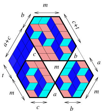
Figure 1.4: Partitioning the compound box into three rectangular boxes in the case of x=y=z=0๐‘ฅ๐‘ฆ๐‘ง0x=y=z=0.

One readily sees that MacMahonโ€™s classical theorem (1.1) is a special case of Theorem 1.2, when m=a=b=c=0๐‘š๐‘Ž๐‘๐‘0m=a=b=c=0, i.e.

Fโ€‹(xyzt0000;q)=Pqโ€‹(z,x+y,t),๐นmatrix๐‘ฅ๐‘ฆ๐‘ง๐‘ก0000๐‘žsubscript๐‘ƒ๐‘ž๐‘ง๐‘ฅ๐‘ฆ๐‘กF\left(\begin{matrix}x&y&z&t\\ 0&0&0&0\end{matrix}\ ;\ q\right)=P_{q}(z,x+y,t), (1.7)

where Pqโ€‹(a,b,c)subscript๐‘ƒ๐‘ž๐‘Ž๐‘๐‘P_{q}(a,b,c) denotes the MacMahon generating function in (1.1). In addition to the above โ€˜naturalโ€™ reduction, the opposite extreme case of x=y=z=0๐‘ฅ๐‘ฆ๐‘ง0x=y=z=0 is also interesting, since it gives a reduction to a product of three MacMahon generating functions, i.e.,

Fโ€‹(000tmabc;q)=Pqโ€‹(a,c,m)โ€‹Pqโ€‹(b,m,c+t)โ€‹Pqโ€‹(m,b,a).๐นmatrix000๐‘ก๐‘š๐‘Ž๐‘๐‘๐‘žsubscript๐‘ƒ๐‘ž๐‘Ž๐‘๐‘šsubscript๐‘ƒ๐‘ž๐‘๐‘š๐‘๐‘กsubscript๐‘ƒ๐‘ž๐‘š๐‘๐‘ŽF\left(\begin{matrix}0&0&0&t\\ m&a&b&c\end{matrix}\ ;\ q\right)=P_{q}(a,c,m)P_{q}(b,m,c+t)P_{q}(m,b,a). (1.8)

In this case, the compound box โ„ฌโ€‹(000tmabc)โ„ฌmatrix000๐‘ก๐‘š๐‘Ž๐‘๐‘\mathcal{B}\begin{pmatrix}0&0&0&t\\ m&a&b&c\end{pmatrix} is a union of three face-disjoint component boxes: the box 111, the box 333, and the box 666, as indexed in Figure 1.3 (the three other boxes are now empty). Therefore, each generalized plane partition fitting in the compound box is now a union of three independent piles of unit cubes fitting in the above three component boxes (see the three boxes corresponding the hexagons with the bold boundary in Figure 1.4). The identity (1.8) then follows. Hence, the main result of this paper can also be regarded as a generalization of three simultaneous instances of MacMahonโ€™s theorem. The unweighted version of (1.8) (when t=0๐‘ก0t=0) also applies to the main result of Ciucuโ€“Krattenthaler [8], as pointed out in their Remark 1 and Figure 8.

It is worth noticing that Ciucu and Krattenthaler [8] proved a closed form product formula for the number of tilings of a hexagon with a shamrock hole in the center. However, there are not any q๐‘žq-enumerations presented in [8].

The goal of the present paper is proving Theorem 1.2 by using the graphical condensation method first introduced by Eric H. Kuo in [19]. This condensation can be viewed as a combinatorial interpretation of Dodgson condensation (which is based on the Jacobi-Desnanot identity, see e.g. [11] and [30], pp. 136โ€“148). We refer the reader to e.g. [4], [12], [20], [35], [38], [39] for various aspects and generalizations of the method; and e.g. [7], [6], [8], [9], [17], [22], [23], [24], [25], [26], [27], [28], [31], [32], [40] for recent applications of Kuo condensation.

The rest of our paper is organized as follows. For ease of reference, we quote several preliminary results in Section 2, including the particular version of Kuo condensation employed in our proofs. In order to apply Kuo condensation to our Q๐‘„Q-type regions, we consider several simple weight assignments on the lozenges of the regions in Section 3. Section 4 is devoted to two generalizations of related work of Ciucu and Krattenthaler in [8, Theorem 3.1] about the magnet bar region (the b=c=0๐‘๐‘0b=c=0 specialization of a Q๐‘„Q-type region). Finally, we prove Theorem 1.2 in Section 5.

2 Preliminaries

Let G๐บG be a finite simple graph without loops. A perfect matching of G๐บG is a collection of edges covering each vertex of G๐บG exactly once. Let R๐‘…R be a region333From now on, we use the word region to mean a finite connected region on the triangular lattice.. The (planar) dual graph of R๐‘…R is the graph whose vertices are unit triangles in R๐‘…R and whose edges connect precisely two unit triangles sharing an edge. One can identify the lozenge tilings of R๐‘…R with the perfect matchings of its dual graph.

For a weighted graph G๐บG, we define the matching generating function Mโก(G)M๐บ\operatorname{M}(G) of G๐บG to be the sum of the weights of all perfect matchings in G๐บG, where the weight of a perfect matching is the product of weights of its edges. If the lozenges of a region R๐‘…R are weighted, we define similarly the tiling generating function Mโก(R)M๐‘…\operatorname{M}(R) of R๐‘…R. In the weighted case, each edge of the dual graph G๐บG of the region R๐‘…R carries the same weight as its corresponding lozenge in R๐‘…R.

The following condensation theorem by Kuo is the key for our proofs.

Theorem 2.3 (Theorem 5.1 in [19]).

Let G=(V1,V2,E)๐บsubscript๐‘‰1subscript๐‘‰2๐ธG=(V_{1},V_{2},E) be a (weighted) bipartite planar graph in which |V1|=|V2|subscript๐‘‰1subscript๐‘‰2|V_{1}|=|V_{2}|. Assume that u,v,w,s๐‘ข๐‘ฃ๐‘ค๐‘ u,v,w,s are four vertices appearing in a cyclic order on a face of G๐บG, such that u,wโˆˆV1๐‘ข๐‘คsubscript๐‘‰1u,w\in V_{1} and v,sโˆˆV2๐‘ฃ๐‘ subscript๐‘‰2v,s\in V_{2}. Then

Mโก(G)โ€‹Mโก(Gโˆ’{u,v,w,s})=Mโก(Gโˆ’{u,v})โ€‹Mโก(Gโˆ’{w,s})+Mโก(Gโˆ’{u,s})โ€‹Mโก(Gโˆ’{v,w}).M๐บM๐บ๐‘ข๐‘ฃ๐‘ค๐‘ M๐บ๐‘ข๐‘ฃM๐บ๐‘ค๐‘ M๐บ๐‘ข๐‘ M๐บ๐‘ฃ๐‘ค\operatorname{M}(G)\operatorname{M}(G-\{u,v,w,s\})=\operatorname{M}(G-\{u,v\})\operatorname{M}(G-\{w,s\})+\operatorname{M}(G-\{u,s\})\operatorname{M}(G-\{v,w\}). (2.1)

A forced lozenge of a region R๐‘…R is a lozenge that is contained in every tiling of R๐‘…R. Assume that we removed several forced lozenges โ„“1,โ„“2,โ€ฆ,โ„“nsubscriptโ„“1subscriptโ„“2โ€ฆsubscriptโ„“๐‘›\ell_{1},\ell_{2},\dotsc,\ell_{n} from the region R๐‘…R, and denote by Rโ€ฒsuperscript๐‘…โ€ฒR^{\prime} the resulting region. Then one clearly has

Mโก(R)=Mโก(Rโ€ฒ)โ€‹โˆi=1nwโ€‹tโ€‹(โ„“i),M๐‘…Msuperscript๐‘…โ€ฒsuperscriptsubscriptproduct๐‘–1๐‘›๐‘ค๐‘กsubscriptโ„“๐‘–\operatorname{M}(R)=\operatorname{M}(R^{\prime})\prod_{i=1}^{n}wt(\ell_{i}), (2.2)

where wโ€‹tโ€‹(โ„“i)๐‘ค๐‘กsubscriptโ„“๐‘–wt(\ell_{i}) denotes the weight of the lozenge โ„“isubscriptโ„“๐‘–\ell_{i}.

If a region R๐‘…R admits a lozenge tiling, then the number of up-pointing unit triangles equals the number of down-pointing unit triangles in R๐‘…R. If a region satisfies the latter balancing condition, we say that the region is balanced. The following lemma can be considered as a generalization of the identity (2.2).

Lemma 2.4 (Region-splitting Lemma).

Let R๐‘…R be a balanced region. Assume that a subregion S๐‘†S of R๐‘…R satisfies the following two conditions:

  1. (i)

    (Separating Condition) There is only one type of unit triangle (up-pointing or down-pointing) running along each side of the border between S๐‘†S and Rโˆ’S๐‘…๐‘†R-S.

  2. (ii)

    (Balancing Condition) S๐‘†S is balanced.

Then

Mโก(R)=Mโก(S)โ€‹Mโก(Rโˆ’S).M๐‘…M๐‘†M๐‘…๐‘†\operatorname{M}(R)=\operatorname{M}(S)\,\operatorname{M}(R-S). (2.3)
Proof.

Assume there is a tiling of R๐‘…R which contains boundary-crossing lozenges between S๐‘†S and Rโˆ’S๐‘…๐‘†R-S (i.e., lozenges which consist of a unit triangle from the boundary of S๐‘†S and a unit triangle from the boundary of Rโˆ’S๐‘…๐‘†R-S). Since there is only one type of unit triangle on each side of the boundary between S๐‘†S and Rโˆ’S๐‘…๐‘†R-S, and since S๐‘†S and Rโˆ’S๐‘…๐‘†R-S are balanced, the regions obtained by removing such boundary-crossing lozenges would no longer be balanced, and hence would have no tilings. Therefore, there can not be any boundary-crossing lozenges, and S๐‘†S and Rโˆ’S๐‘…๐‘†R-S must be tiled independently, giving the factorization (2.3). โˆŽ

3 q๐‘žq-weight assignments

Lozenges in a region R๐‘…R come with three different orientations: left, right, and vertical lozenges (see Figure 3.1). Next, we consider three simple q๐‘žq-weight assignments of lozenges in our region Q:=Qโ€‹(xyztmabc)assign๐‘„๐‘„matrix๐‘ฅ๐‘ฆ๐‘ง๐‘ก๐‘š๐‘Ž๐‘๐‘Q:=Q\begin{pmatrix}x&y&z&t\\ m&a&b&c\end{pmatrix} as follows.

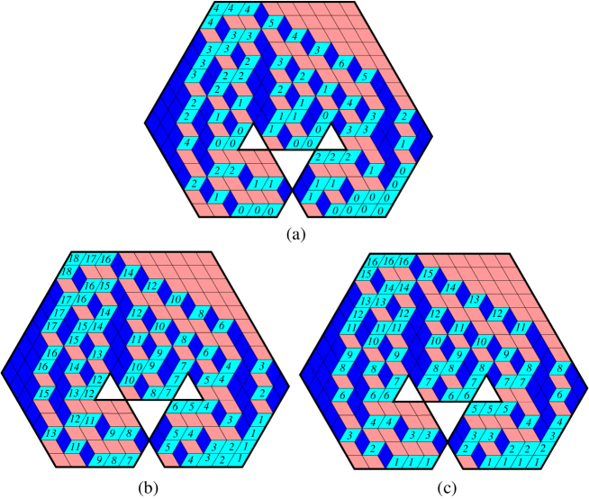
View a lozenge tiling T๐‘‡T of the region Q๐‘„Q as a generalized plane partition (i.e. a pile of unit cubes); each right lozenge is viewed as the top of a column of unit cubes. We assign to each right lozenge the weight qxsuperscript๐‘ž๐‘ฅq^{x}, where x๐‘ฅx is the number of unit cubes in the corresponding column. All left and vertical lozenges are weighted by 111. We call this assignment the natural q-weight assignment of Q๐‘„Q, and use the notation wโ€‹t0๐‘คsubscript๐‘ก0wt_{0} for the assignment (see Figure 3.2(a) for the case when x=y=z=3๐‘ฅ๐‘ฆ๐‘ง3x=y=z=3, t=4๐‘ก4t=4, m=3๐‘š3m=3, a=b=c=2๐‘Ž๐‘๐‘2a=b=c=2).

Refer to caption
Figure 3.1: Three orientations of lozenges.
Refer to caption
Figure 3.2: Three q๐‘žq-weight assignments on a sample tiling of region Q๐‘„Q: (a) wโ€‹t0๐‘คsubscript๐‘ก0wt_{0}, (b) wโ€‹t1๐‘คsubscript๐‘ก1wt_{1}, (c) wโ€‹t2๐‘คsubscript๐‘ก2wt_{2}. The right lozenges with label x๐‘ฅx are weighted by qxsuperscript๐‘ž๐‘ฅq^{x}.

Besides the natural q๐‘žq-weight assignment wโ€‹t0๐‘คsubscript๐‘ก0wt_{0}, we consider the following two q๐‘žq-weight assignments:

  1. (1)

    Assignment 1. The weights of left and vertical lozenges are all 1. The weight of a right lozenge is qlsuperscript๐‘ž๐‘™q^{l}, where l๐‘™l is the distance between the left side of the lozenge and the southeast side of the region Q๐‘„Q. We use notation wโ€‹t1๐‘คsubscript๐‘ก1wt_{1} for this weight assignment (see Figure 3.2(b)).

  2. (2)

    Assignment 2. All left and vertical lozenges are also weighted by 1. However, a right lozenge is now weighted by qnsuperscript๐‘ž๐‘›q^{n}, where n๐‘›n is the distance between the top of the lozenge and the base of the region Q๐‘„Q. This assignment is denoted by wโ€‹t2๐‘คsubscript๐‘ก2wt_{2} (see Figure 3.2(c)).

Let T๐‘‡T be a tiling of Q๐‘„Q. We denote by wโ€‹t0โ€‹(T)๐‘คsubscript๐‘ก0๐‘‡wt_{0}(T), wโ€‹t1โ€‹(T)๐‘คsubscript๐‘ก1๐‘‡wt_{1}(T) and wโ€‹t2โ€‹(T)๐‘คsubscript๐‘ก2๐‘‡wt_{2}(T) the weights of the tiling T๐‘‡T with respect to the weight assignments wโ€‹t0๐‘คsubscript๐‘ก0wt_{0}, wโ€‹t1๐‘คsubscript๐‘ก1wt_{1} and wโ€‹t2๐‘คsubscript๐‘ก2wt_{2}. We also denote by M0โก(Q)subscriptM0๐‘„\operatorname{M}_{0}(Q), M1โก(Q)subscriptM1๐‘„\operatorname{M}_{1}(Q) and M2โก(Q)subscriptM2๐‘„\operatorname{M}_{2}(Q) the tiling generating functions of Q๐‘„Q corresponding to the weight assignments wโ€‹t0๐‘คsubscript๐‘ก0wt_{0}, wโ€‹t1๐‘คsubscript๐‘ก1wt_{1} and wโ€‹t2๐‘คsubscript๐‘ก2wt_{2}. It is easy to see that M0โก(Q)subscriptM0๐‘„\operatorname{M}_{0}(Q) is exactly the volume generation function of the generalized plane partitions corresponding to the lozenge tilings of Q๐‘„Q.

In the next proposition, we will show that the three weight assignments are the same up to some multiplicative factors.

We define two functions

f (xyztmabc):=mโ€‹(y+b+12)+zโ€‹(y+12)+mโ€‹(z+b)โ€‹(y+a+b)+(z+b)โ€‹(m+12)assignmatrix๐‘ฅ๐‘ฆ๐‘ง๐‘ก๐‘š๐‘Ž๐‘๐‘๐‘šbinomial๐‘ฆ๐‘12๐‘งbinomial๐‘ฆ12๐‘š๐‘ง๐‘๐‘ฆ๐‘Ž๐‘๐‘ง๐‘binomial๐‘š12\displaystyle\begin{pmatrix}x&y&z&t\\ m&a&b&c\end{pmatrix}:=m\binom{y+b+1}{2}+z\binom{y+1}{2}+m(z+b)(y+a+b)+(z+b)\binom{m+1}{2}
+xโ€‹(z+b+c)โ€‹(y+m+a+b+c)+(z+b+c)โ€‹(x+12)+aโ€‹(x+c)โ€‹(y+a+b)+aโ€‹(x+c+12)๐‘ฅ๐‘ง๐‘๐‘๐‘ฆ๐‘š๐‘Ž๐‘๐‘๐‘ง๐‘๐‘binomial๐‘ฅ12๐‘Ž๐‘ฅ๐‘๐‘ฆ๐‘Ž๐‘๐‘Žbinomial๐‘ฅ๐‘12\displaystyle+x(z+b+c)(y+m+a+b+c)+(z+b+c)\binom{x+1}{2}+a(x+c)(y+a+b)+a\binom{x+c+1}{2} (3.1)

and

g (xyztmabc):=(y+b)โ€‹(m+12)+mโ€‹yโ€‹z+yโ€‹(z+12)+mโ€‹(z+b)โ€‹(m+a)assignmatrix๐‘ฅ๐‘ฆ๐‘ง๐‘ก๐‘š๐‘Ž๐‘๐‘๐‘ฆ๐‘binomial๐‘š12๐‘š๐‘ฆ๐‘ง๐‘ฆbinomial๐‘ง12๐‘š๐‘ง๐‘๐‘š๐‘Ž\displaystyle\begin{pmatrix}x&y&z&t\\ m&a&b&c\end{pmatrix}:=(y+b)\binom{m+1}{2}+myz+y\binom{z+1}{2}+m(z+b)(m+a)
+mโ€‹(z+b+12)+xโ€‹(m+a)โ€‹(z+b+c)+xโ€‹(z+b+c+12)+(x+c)โ€‹(a+12).๐‘šbinomial๐‘ง๐‘12๐‘ฅ๐‘š๐‘Ž๐‘ง๐‘๐‘๐‘ฅbinomial๐‘ง๐‘๐‘12๐‘ฅ๐‘binomial๐‘Ž12\displaystyle+m\binom{z+b+1}{2}+x(m+a)(z+b+c)+x\binom{z+b+c+1}{2}+(x+c)\binom{a+1}{2}. (3.2)

Note that fโ€‹(xyztmabc)fmatrix๐‘ฅ๐‘ฆ๐‘ง๐‘ก๐‘š๐‘Ž๐‘๐‘\textbf{f}\begin{pmatrix}x&y&z&t\\ m&a&b&c\end{pmatrix} and gโ€‹(xyztmabc)gmatrix๐‘ฅ๐‘ฆ๐‘ง๐‘ก๐‘š๐‘Ž๐‘๐‘\textbf{g}\begin{pmatrix}x&y&z&t\\ m&a&b&c\end{pmatrix} are both independent of t๐‘กt.

Proposition 3.5.

For any non-negative integers m,a,b,c,x,y,z,t๐‘š๐‘Ž๐‘๐‘๐‘ฅ๐‘ฆ๐‘ง๐‘กm,a,b,c,x,y,z,t

M1โก(Qโ€‹(xyztmabc))=qfโ€‹(xyztmabc)โ€‹โˆ‘ฯ€q|ฯ€|subscriptM1๐‘„matrix๐‘ฅ๐‘ฆ๐‘ง๐‘ก๐‘š๐‘Ž๐‘๐‘superscript๐‘žfmatrix๐‘ฅ๐‘ฆ๐‘ง๐‘ก๐‘š๐‘Ž๐‘๐‘subscript๐œ‹superscript๐‘ž๐œ‹\operatorname{M}_{1}\left(Q\begin{pmatrix}x&y&z&t\\ m&a&b&c\end{pmatrix}\right)=q^{\textbf{f}\begin{pmatrix}x&y&z&t\\ m&a&b&c\end{pmatrix}}\sum_{\pi}q^{|\pi|} (3.3)

and

M2โก(Qโ€‹(xyztmabc))=qgโ€‹(xyztmabc)โ€‹โˆ‘ฯ€q|ฯ€|,subscriptM2๐‘„matrix๐‘ฅ๐‘ฆ๐‘ง๐‘ก๐‘š๐‘Ž๐‘๐‘superscript๐‘žgmatrix๐‘ฅ๐‘ฆ๐‘ง๐‘ก๐‘š๐‘Ž๐‘๐‘subscript๐œ‹superscript๐‘ž๐œ‹\operatorname{M}_{2}\left(Q\begin{pmatrix}x&y&z&t\\ m&a&b&c\end{pmatrix}\right)=q^{\textbf{g}\begin{pmatrix}x&y&z&t\\ m&a&b&c\end{pmatrix}}\sum_{\pi}q^{|\pi|}, (3.4)

where the sums on the right-hand sides are taken over all generalized plane partitions ฯ€๐œ‹\pi fitting in the compound box โ„ฌโ€‹(xyztmabc)โ„ฌmatrix๐‘ฅ๐‘ฆ๐‘ง๐‘ก๐‘š๐‘Ž๐‘๐‘\mathcal{B}\begin{pmatrix}x&y&z&t\\ m&a&b&c\end{pmatrix}.

Refer to caption
Figure 3.3: The partial-partition corresponding to the box 333.
Proof.

We use the following shorthand notations in this proof: f:=fโ€‹(xyztmabc)assignffmatrix๐‘ฅ๐‘ฆ๐‘ง๐‘ก๐‘š๐‘Ž๐‘๐‘\textbf{f}:=\textbf{f}\begin{pmatrix}x&y&z&t\\ m&a&b&c\end{pmatrix}, g:=gโ€‹(xyztmabc)assignggmatrix๐‘ฅ๐‘ฆ๐‘ง๐‘ก๐‘š๐‘Ž๐‘๐‘\textbf{g}:=\textbf{g}\begin{pmatrix}x&y&z&t\\ m&a&b&c\end{pmatrix}, โ„ฌ:=โ„ฌโ€‹(xyztmabc)assignโ„ฌโ„ฌmatrix๐‘ฅ๐‘ฆ๐‘ง๐‘ก๐‘š๐‘Ž๐‘๐‘\mathcal{B}:=\mathcal{B}\begin{pmatrix}x&y&z&t\\ m&a&b&c\end{pmatrix}, and Q:=Qโ€‹(xyztmabc)assign๐‘„๐‘„matrix๐‘ฅ๐‘ฆ๐‘ง๐‘ก๐‘š๐‘Ž๐‘๐‘Q:=Q\begin{pmatrix}x&y&z&t\\ m&a&b&c\end{pmatrix}.

Let T๐‘‡T be any lozenge tiling of the region Q๐‘„Q, and ฯ€๐œ‹\pi the generalized plane partition corresponding to T๐‘‡T. We only need to show that

wโ€‹t1โ€‹(T)q|ฯ€|=qfย andย wโ€‹t2โ€‹(T)q|ฯ€|=qg.formulae-sequence๐‘คsubscript๐‘ก1๐‘‡superscript๐‘ž๐œ‹superscript๐‘žfย andย ๐‘คsubscript๐‘ก2๐‘‡superscript๐‘ž๐œ‹superscript๐‘žg\frac{wt_{1}(T)}{q^{|\pi|}}=q^{\textbf{f}}\quad\text{ and }\quad\frac{wt_{2}(T)}{q^{|\pi|}}=q^{\textbf{g}}. (3.5)

Assume that the box i๐‘–i of the compound box โ„ฌโ„ฌ\mathcal{B} has size aiร—biร—cisubscript๐‘Ž๐‘–subscript๐‘๐‘–subscript๐‘๐‘–a_{i}\times b_{i}\times c_{i} (for 1โ‰คiโ‰ค61๐‘–61\leq i\leq 6). The base of the box i๐‘–i is depicted as a parallelogram Pisubscript๐‘ƒ๐‘–P_{i} consisting of right lozenges in Figure 1.3(b). We assume in addition that the left side of Pisubscript๐‘ƒ๐‘–P_{i} is xisubscript๐‘ฅ๐‘–x_{i} units to the left of the southeast side of the region Q๐‘„Q, and the bottom of Pisubscript๐‘ƒ๐‘–P_{i} is yisubscript๐‘ฆ๐‘–y_{i} units above the bottom of region Q๐‘„Q.

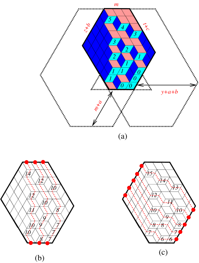
Divide the generalized plane partition ฯ€๐œ‹\pi into 666 disjoint partial-partitions ฯ€isubscript๐œ‹๐‘–\pi_{i} (1โ‰คiโ‰ค61๐‘–61\leq i\leq 6) fitting in the box i๐‘–i. Recall that the box i๐‘–i is associated with a semi-regular hexagon with side lengths aisubscript๐‘Ž๐‘–a_{i}, bisubscript๐‘๐‘–b_{i}, cisubscript๐‘๐‘–c_{i}, aisubscript๐‘Ž๐‘–a_{i}, bisubscript๐‘๐‘–b_{i}, cisubscript๐‘๐‘–c_{i}, in clockwise order from the northwest side. Each partial-partition ฯ€isubscript๐œ‹๐‘–\pi_{i} in turn gives a lozenge tiling Tisubscript๐‘‡๐‘–T_{i} of the semi-regular hexagon Hโ€‹eโ€‹xโ€‹(ai,bi,ci)๐ป๐‘’๐‘ฅsubscript๐‘Ž๐‘–subscript๐‘๐‘–subscript๐‘๐‘–Hex(a_{i},b_{i},c_{i}). Figure 3.3(a) shows the partial-partition ฯ€3subscript๐œ‹3\pi_{3} of the generalized plane partition ฯ€๐œ‹\pi in Figure 1.3(a), as well as the relative positions of the parallelogram P3subscript๐‘ƒ3P_{3} to the bottom and the southeast side of the region Q๐‘„Q (for x=3,y=3,z=3,t=4,m=3,a=2,b=2,c=2formulae-sequence๐‘ฅ3formulae-sequence๐‘ฆ3formulae-sequence๐‘ง3formulae-sequence๐‘ก4formulae-sequence๐‘š3formulae-sequence๐‘Ž2formulae-sequence๐‘2๐‘2x=3,y=3,z=3,t=4,m=3,a=2,b=2,c=2). In particular, this gives a3=z+bsubscript๐‘Ž3๐‘ง๐‘a_{3}=z+b, b3=msubscript๐‘3๐‘šb_{3}=m, c3=t+csubscript๐‘3๐‘ก๐‘c_{3}=t+c, x3=y+a+bsubscript๐‘ฅ3๐‘ฆ๐‘Ž๐‘x_{3}=y+a+b and y3=m+asubscript๐‘ฆ3๐‘š๐‘Žy_{3}=m+a.

Apply the weight assignment wโ€‹t1๐‘คsubscript๐‘ก1wt_{1} to the whole tiling T๐‘‡T of the region Q๐‘„Q. This yields a local weight assignment wโ€‹t1(i)๐‘คsuperscriptsubscript๐‘ก1๐‘–wt_{1}^{(i)} for the tiling Tisubscript๐‘‡๐‘–T_{i} of hexagon Hโ€‹eโ€‹xโ€‹(ai,bi,ci)๐ป๐‘’๐‘ฅsubscript๐‘Ž๐‘–subscript๐‘๐‘–subscript๐‘๐‘–Hex(a_{i},b_{i},c_{i}). Precisely, each right lozenge in Tisubscript๐‘‡๐‘–T_{i} is now weighted by qxi+lsuperscript๐‘žsubscript๐‘ฅ๐‘–๐‘™q^{x_{i}+l}, where l๐‘™l is the distance between the left side of the lozenge and the southeast side of the hexagon Hโ€‹eโ€‹xโ€‹(ai,bi,ci)๐ป๐‘’๐‘ฅsubscript๐‘Ž๐‘–subscript๐‘๐‘–subscript๐‘๐‘–Hex(a_{i},b_{i},c_{i}). Encode the tiling Tisubscript๐‘‡๐‘–T_{i} as a family of bisubscript๐‘๐‘–b_{i} disjoint lozenge-paths connecting the top and the bottom of the hexagon (see the dotted paths in Figure 3.3(b)). Dividing the weight of each right lozenge in the lozenge-path j๐‘—j (from right to left) by qxi+jsuperscript๐‘žsubscript๐‘ฅ๐‘–๐‘—q^{x_{i}+j}, we get the weight assignment wโ€‹t0๐‘คsubscript๐‘ก0wt_{0} for Tisubscript๐‘‡๐‘–T_{i}. Since the end points of the above lozenge-paths are fixed, each lozenge-path has exactly aisubscript๐‘Ž๐‘–a_{i} right lozenges. Thus, we have

wโ€‹t1(i)โ€‹(Ti)wโ€‹t0โ€‹(Ti)=wโ€‹t1(i)โ€‹(Ti)q|ฯ€i|=qaiโ€‹biโ€‹xi+aiโ€‹biโ€‹(bi+1)/2.๐‘คsuperscriptsubscript๐‘ก1๐‘–subscript๐‘‡๐‘–๐‘คsubscript๐‘ก0subscript๐‘‡๐‘–๐‘คsuperscriptsubscript๐‘ก1๐‘–subscript๐‘‡๐‘–superscript๐‘žsubscript๐œ‹๐‘–superscript๐‘žsubscript๐‘Ž๐‘–subscript๐‘๐‘–subscript๐‘ฅ๐‘–subscript๐‘Ž๐‘–subscript๐‘๐‘–subscript๐‘๐‘–12\frac{wt_{1}^{(i)}(T_{i})}{wt_{0}(T_{i})}=\frac{wt_{1}^{(i)}(T_{i})}{q^{|\pi_{i}|}}=q^{a_{i}b_{i}x_{i}+a_{i}b_{i}(b_{i}+1)/2}.

Multiplying all above equations for i=1,2,โ€ฆ,6๐‘–12โ€ฆ6i=1,2,\dotsc,6, we get

wโ€‹t1โ€‹(T)q|ฯ€|=qโˆ‘i=16(aiโ€‹biโ€‹xi+aiโ€‹biโ€‹(bi+1)/2).๐‘คsubscript๐‘ก1๐‘‡superscript๐‘ž๐œ‹superscript๐‘žsuperscriptsubscript๐‘–16subscript๐‘Ž๐‘–subscript๐‘๐‘–subscript๐‘ฅ๐‘–subscript๐‘Ž๐‘–subscript๐‘๐‘–subscript๐‘๐‘–12\frac{wt_{1}(T)}{q^{|\pi|}}=q^{\sum_{i=1}^{6}(a_{i}b_{i}x_{i}+a_{i}b_{i}(b_{i}+1)/2)}. (3.6)

Next, we assume that the whole tiling T๐‘‡T of Q๐‘„Q is weighted by wโ€‹t2๐‘คsubscript๐‘ก2wt_{2}. We now encode the tiling Tisubscript๐‘‡๐‘–T_{i} of Hโ€‹eโ€‹xโ€‹(ai,bi,ci)๐ป๐‘’๐‘ฅsubscript๐‘Ž๐‘–subscript๐‘๐‘–subscript๐‘๐‘–Hex(a_{i},b_{i},c_{i}) as an aisubscript๐‘Ž๐‘–a_{i}-tuple of disjoint lozenge-paths connecting the northwest side and the southeast side of the hexagon (see Figure 3.3(c)). Dividing each right lozenge in the lozenge-path j๐‘—j (from bottom to top) by qyi+jsuperscript๐‘žsubscript๐‘ฆ๐‘–๐‘—q^{y_{i}+j}, we get back again the weight assignment wโ€‹t0๐‘คsubscript๐‘ก0wt_{0}. We note that each lozenge-path has now bisubscript๐‘๐‘–b_{i} right lozenges. Similar to the case of wโ€‹t1๐‘คsubscript๐‘ก1wt_{1}, we have

wโ€‹t2โ€‹(T)q|ฯ€|=qโˆ‘i=16(aiโ€‹biโ€‹yi+biโ€‹aiโ€‹(ai+1)/2).๐‘คsubscript๐‘ก2๐‘‡superscript๐‘ž๐œ‹superscript๐‘žsuperscriptsubscript๐‘–16subscript๐‘Ž๐‘–subscript๐‘๐‘–subscript๐‘ฆ๐‘–subscript๐‘๐‘–subscript๐‘Ž๐‘–subscript๐‘Ž๐‘–12\frac{wt_{2}(T)}{q^{|\pi|}}=q^{\sum_{i=1}^{6}(a_{i}b_{i}y_{i}+b_{i}a_{i}(a_{i}+1)/2)}. (3.7)

Obtaining the formulas for ai,bi,xi,yisubscript๐‘Ž๐‘–subscript๐‘๐‘–subscript๐‘ฅ๐‘–subscript๐‘ฆ๐‘–a_{i},b_{i},x_{i},y_{i} in terms of m,a,b,c,x,y,z,t๐‘š๐‘Ž๐‘๐‘๐‘ฅ๐‘ฆ๐‘ง๐‘กm,a,b,c,x,y,z,t from Figures 1.3(b) and (c), we get f=โˆ‘i=16(aiโ€‹biโ€‹xi+aiโ€‹biโ€‹(bi+1)/2)fsuperscriptsubscript๐‘–16subscript๐‘Ž๐‘–subscript๐‘๐‘–subscript๐‘ฅ๐‘–subscript๐‘Ž๐‘–subscript๐‘๐‘–subscript๐‘๐‘–12\textbf{f}=\sum_{i=1}^{6}(a_{i}b_{i}x_{i}+a_{i}b_{i}(b_{i}+1)/2) and g=โˆ‘i=16(aiโ€‹biโ€‹yi+biโ€‹aiโ€‹(ai+1)/2)gsuperscriptsubscript๐‘–16subscript๐‘Ž๐‘–subscript๐‘๐‘–subscript๐‘ฆ๐‘–subscript๐‘๐‘–subscript๐‘Ž๐‘–subscript๐‘Ž๐‘–12\textbf{g}=\sum_{i=1}^{6}(a_{i}b_{i}y_{i}+b_{i}a_{i}(a_{i}+1)/2). This finishes our proof. โˆŽ

We note that the powers qfsuperscript๐‘žfq^{\textbf{f}} and qgsuperscript๐‘žgq^{\textbf{g}} in the above proposition are exactly the weights wโ€‹t1โ€‹(T0)๐‘คsubscript๐‘ก1subscript๐‘‡0wt_{1}(T_{0}) and wโ€‹t2โ€‹(T0)๐‘คsubscript๐‘ก2subscript๐‘‡0wt_{2}(T_{0}) of the tiling T0subscript๐‘‡0T_{0} corresponding to the empty pile in Figure 1.3(b).

View the hexagon Hโ€‹eโ€‹xโ€‹(a,b,c)๐ป๐‘’๐‘ฅ๐‘Ž๐‘๐‘Hex(a,b,c) as a special case of the region Q:=Qโ€‹(xyztmabc)assign๐‘„๐‘„matrix๐‘ฅ๐‘ฆ๐‘ง๐‘ก๐‘š๐‘Ž๐‘๐‘Q:=Q\begin{pmatrix}x&y&z&t\\ m&a&b&c\end{pmatrix} with an empty shamrock hole, i.e., set m=a=b=c=0๐‘š๐‘Ž๐‘๐‘0m=a=b=c=0, and then replace z๐‘งz, x+y๐‘ฅ๐‘ฆx+y and t๐‘กt by a,๐‘Ža, b๐‘b and c๐‘c, respectively. We then have the following consequence of Proposition 3.5 and MacMahonโ€™s q๐‘žq-formula (1.1).

Corollary 3.6.

For non-negative integers a,b,c๐‘Ž๐‘๐‘a,b,c

M1โก(Hโ€‹eโ€‹xโ€‹(a,b,c))=qaโ€‹bโ€‹(b+1)/2โ€‹Hqโก(a)โ€‹Hqโก(b)โ€‹Hqโก(c)โ€‹Hqโก(a+b+c)Hqโก(a+b)โ€‹Hqโก(b+c)โ€‹Hqโก(c+a)subscriptM1๐ป๐‘’๐‘ฅ๐‘Ž๐‘๐‘superscript๐‘ž๐‘Ž๐‘๐‘12subscriptH๐‘ž๐‘ŽsubscriptH๐‘ž๐‘subscriptH๐‘ž๐‘subscriptH๐‘ž๐‘Ž๐‘๐‘subscriptH๐‘ž๐‘Ž๐‘subscriptH๐‘ž๐‘๐‘subscriptH๐‘ž๐‘๐‘Ž\operatorname{M}_{1}\big{(}Hex(a,b,c)\big{)}=q^{ab(b+1)/2}\frac{\operatorname{H}_{q}(a)\operatorname{H}_{q}(b)\operatorname{H}_{q}(c)\operatorname{H}_{q}(a+b+c)}{\operatorname{H}_{q}(a+b)\operatorname{H}_{q}(b+c)\operatorname{H}_{q}(c+a)} (3.8)

and

M2โก(Hโ€‹eโ€‹xโ€‹(a,b,c))=qbโ€‹aโ€‹(a+1)/2โ€‹Hqโก(a)โ€‹Hqโก(b)โ€‹Hqโก(c)โ€‹Hqโก(a+b+c)Hqโก(a+b)โ€‹Hqโก(b+c)โ€‹Hqโก(c+a).subscriptM2๐ป๐‘’๐‘ฅ๐‘Ž๐‘๐‘superscript๐‘ž๐‘๐‘Ž๐‘Ž12subscriptH๐‘ž๐‘ŽsubscriptH๐‘ž๐‘subscriptH๐‘ž๐‘subscriptH๐‘ž๐‘Ž๐‘๐‘subscriptH๐‘ž๐‘Ž๐‘subscriptH๐‘ž๐‘๐‘subscriptH๐‘ž๐‘๐‘Ž\operatorname{M}_{2}\big{(}Hex(a,b,c)\big{)}=q^{ba(a+1)/2}\frac{\operatorname{H}_{q}(a)\operatorname{H}_{q}(b)\operatorname{H}_{q}(c)\operatorname{H}_{q}(a+b+c)}{\operatorname{H}_{q}(a+b)\operatorname{H}_{q}(b+c)\operatorname{H}_{q}(c+a)}. (3.9)

The following definitions will be used in the proof of the next lemma. A column-strict plane partition is a plane partition having columns strictly decreasing. A semihexagon Sโ€‹Ha,b๐‘†subscript๐ป๐‘Ž๐‘SH_{a,b} is the upper half of a lozenge hexagon Hโ€‹eโ€‹xโ€‹(a,b,a)๐ป๐‘’๐‘ฅ๐‘Ž๐‘๐‘ŽHex(a,b,a). We are interested in the lozenge tilings of the semihexagon Sโ€‹Ha,b๐‘†subscript๐ป๐‘Ž๐‘SH_{a,b}, where a๐‘Ža up-pointing unit triangles at the positions s1,s2,โ€ฆ,sasubscript๐‘ 1subscript๐‘ 2โ€ฆsubscript๐‘ ๐‘Žs_{1},s_{2},\dots,s_{a} have been removed from the base. Denote by Sโ€‹Ha,bโ€‹(s1,s2,โ€ฆ,sa)๐‘†subscript๐ป๐‘Ž๐‘subscript๐‘ 1subscript๐‘ 2โ€ฆsubscript๐‘ ๐‘ŽSH_{a,b}(s_{1},s_{2},\dots,s_{a}) the resulting semihexagon with dents (see Figure 3.4(a) for the region Sโ€‹H7,5โ€‹(1,2,6,7,10,11,12)๐‘†subscript๐ป751267101112SH_{7,5}(1,2,6,7,10,11,12)). Assume that the lozenges in the semihexagon are weighted by wโ€‹t2๐‘คsubscript๐‘ก2wt_{2}, and we still use the notation M2subscriptM2\operatorname{M}_{2} for the corresponding tiling generating function of the semihexagon with dents. There is a well-known (weight preserving) bijection between the lozenge tilings of Sโ€‹Ha,bโ€‹(s1,s2,โ€ฆ,sa)๐‘†subscript๐ป๐‘Ž๐‘subscript๐‘ 1subscript๐‘ 2โ€ฆsubscript๐‘ ๐‘ŽSH_{a,b}(s_{1},s_{2},\dots,s_{a}) and the column-strict plane partitions of shape (saโˆ’a,saโˆ’1โˆ’a+1,โ€ฆ,s1โˆ’1)subscript๐‘ ๐‘Ž๐‘Žsubscript๐‘ ๐‘Ž1๐‘Ž1โ€ฆsubscript๐‘ 11(s_{a}-a,s_{a-1}-a+1,\dotsc,s_{1}-1) with positive entries at most a๐‘Ža, i.e. wโ€‹t2โ€‹(T)=q|ฯ€T|๐‘คsubscript๐‘ก2๐‘‡superscript๐‘žsubscript๐œ‹๐‘‡wt_{2}(T)=q^{|\pi_{T}|}, where ฯ€Tsubscript๐œ‹๐‘‡\pi_{T} is the plane partition corresponding to the tiling T๐‘‡T (see e.g. [10] and [1]).

Refer to caption
Figure 3.4: (a) The semihexagon with dents Sโ€‹H7,5โ€‹(1,2,6,7,10,11,12)๐‘†subscript๐ป751267101112SH_{7,5}(1,2,6,7,10,11,12). (b) Obtaining the region Kaโ€‹(x,y,z,t)subscript๐พ๐‘Ž๐‘ฅ๐‘ฆ๐‘ง๐‘กK_{a}(x,y,z,t) (restricted by the bold contour) from a semihexagon with dents by removing forced lozenges.

We have the following q๐‘žq-enumeration of the lozenge tilings of a hexagon with a triangular hole on the base Kaโ€‹(x,y,z,t)subscript๐พ๐‘Ž๐‘ฅ๐‘ฆ๐‘ง๐‘กK_{a}(x,y,z,t) (defined as the region restricted by the bold contour in Figure 3.4(b)). Note that Kaโ€‹(x,y,z,t)subscript๐พ๐‘Ž๐‘ฅ๐‘ฆ๐‘ง๐‘กK_{a}(x,y,z,t) is the region Qโ€‹(xyzt0a00)๐‘„matrix๐‘ฅ๐‘ฆ๐‘ง๐‘ก0๐‘Ž00Q\begin{pmatrix}x&y&z&t\\ 0&a&0&0\end{pmatrix}.

Lemma 3.7.

For non-negative a,x,y,z,t๐‘Ž๐‘ฅ๐‘ฆ๐‘ง๐‘กa,x,y,z,t

M2โก(Kaโ€‹(x,y,z,t))subscriptM2subscript๐พ๐‘Ž๐‘ฅ๐‘ฆ๐‘ง๐‘ก\displaystyle\operatorname{M}_{2}\big{(}K_{a}(x,y,z,t)\big{)} =qyโ€‹(z+12)+xโ€‹(a+z+12)โ€‹Hqโก(a)โ€‹Hqโก(x)โ€‹Hqโก(y)โ€‹Hqโก(z)โ€‹Hqโก(t)Hqโก(x+t)โ€‹Hqโก(a+x)โ€‹Hqโก(a+y)โ€‹Hqโก(y+z)absentsuperscript๐‘ž๐‘ฆbinomial๐‘ง12๐‘ฅbinomial๐‘Ž๐‘ง12subscriptH๐‘ž๐‘ŽsubscriptH๐‘ž๐‘ฅsubscriptH๐‘ž๐‘ฆsubscriptH๐‘ž๐‘งsubscriptH๐‘ž๐‘กsubscriptH๐‘ž๐‘ฅ๐‘กsubscriptH๐‘ž๐‘Ž๐‘ฅsubscriptH๐‘ž๐‘Ž๐‘ฆsubscriptH๐‘ž๐‘ฆ๐‘ง\displaystyle=q^{y\binom{z+1}{2}+x\binom{a+z+1}{2}}\frac{\operatorname{H}_{q}(a)\operatorname{H}_{q}(x)\operatorname{H}_{q}(y)\operatorname{H}_{q}(z)\operatorname{H}_{q}(t)}{\operatorname{H}_{q}(x+t)\operatorname{H}_{q}(a+x)\operatorname{H}_{q}(a+y)\operatorname{H}_{q}(y+z)}
ร—Hqโก(a+x+t)โ€‹Hqโก(a+x+y)โ€‹Hqโก(a+y+z)โ€‹Hqโก(a+x+y+z+t)Hqโก(a+x+y+t)โ€‹Hqโก(a+x+y+z)โ€‹Hqโก(a+t+z).absentsubscriptH๐‘ž๐‘Ž๐‘ฅ๐‘กsubscriptH๐‘ž๐‘Ž๐‘ฅ๐‘ฆsubscriptH๐‘ž๐‘Ž๐‘ฆ๐‘งsubscriptH๐‘ž๐‘Ž๐‘ฅ๐‘ฆ๐‘ง๐‘กsubscriptH๐‘ž๐‘Ž๐‘ฅ๐‘ฆ๐‘กsubscriptH๐‘ž๐‘Ž๐‘ฅ๐‘ฆ๐‘งsubscriptH๐‘ž๐‘Ž๐‘ก๐‘ง\displaystyle\times\frac{\operatorname{H}_{q}(a+x+t)\operatorname{H}_{q}(a+x+y)\operatorname{H}_{q}(a+y+z)\operatorname{H}_{q}(a+x+y+z+t)}{\operatorname{H}_{q}(a+x+y+t)\operatorname{H}_{q}(a+x+y+z)\operatorname{H}_{q}(a+t+z)}. (3.10)
Proof.

By the above bijection between lozenge tilings of the semihexagon and the column-strict plane partitions, we have

M2โก(Sโ€‹Ha,bโ€‹(s1,s2,โ€ฆ,sa))=โˆ‘ฮผq|ฮผ|=qโˆ‘i=1a(siโˆ’i)โ€‹โˆ1โ‰คi<jโ‰คaqsjโˆ’qsiqjโˆ’qi,subscriptM2๐‘†subscript๐ป๐‘Ž๐‘subscript๐‘ 1subscript๐‘ 2โ€ฆsubscript๐‘ ๐‘Žsubscript๐œ‡superscript๐‘ž๐œ‡superscript๐‘žsuperscriptsubscript๐‘–1๐‘Žsubscript๐‘ ๐‘–๐‘–subscriptproduct1๐‘–๐‘—๐‘Žsuperscript๐‘žsubscript๐‘ ๐‘—superscript๐‘žsubscript๐‘ ๐‘–superscript๐‘ž๐‘—superscript๐‘ž๐‘–\operatorname{M}_{2}\big{(}SH_{a,b}(s_{1},s_{2},\dotsc,s_{a})\big{)}=\sum_{\mu}q^{|\mu|}=q^{\sum_{i=1}^{a}(s_{i}-i)}\prod_{1\leq i<j\leq a}\frac{q^{s_{j}}-q^{s_{i}}}{q^{j}-q^{i}}, (3.11)

where the sum after the first equality sign is taken over all column-strict plane partitions ฮผ๐œ‡\mu of shape (saโˆ’a,saโˆ’1โˆ’a+1,โ€ฆ,s1โˆ’1)subscript๐‘ ๐‘Ž๐‘Žsubscript๐‘ ๐‘Ž1๐‘Ž1โ€ฆsubscript๐‘ 11(s_{a}-a,s_{a-1}-a+1,\dotsc,s_{1}-1) with positive entries at most a๐‘Ža. For the second equality see e.g. [37, pp. 374โ€“375].

The region Kaโ€‹(x,y,z,t)subscript๐พ๐‘Ž๐‘ฅ๐‘ฆ๐‘ง๐‘กK_{a}(x,y,z,t) is obtained by removing forced vertical lozenges from the semihexagon Sโ€‹Ha+z+t,x+y๐‘†subscript๐ป๐‘Ž๐‘ง๐‘ก๐‘ฅ๐‘ฆSH_{a+z+t,x+y} with dents at the positions {1,2,..,t}โˆช{t+x+1,t+x+2,โ€ฆ,t+x+a}โˆช{t+x+a+y+1,t+x+a+y+2,โ€ฆ,t+x+a+y+z}\{1,2,..,t\}\cup\{t+x+1,t+x+2,\dotsc,t+x+a\}\cup\{t+x+a+y+1,t+x+a+y+2,\dotsc,t+x+a+y+z\}. Thus, our lemma follows from (3.11). โˆŽ

4 Two q๐‘žq-enumerations of magnet bar regions

Refer to caption
Figure 4.1: The magnet bar B2,2โ€‹(4,3,3,2)subscript๐ต224332B_{2,2}(4,3,3,2).

When b=c=0๐‘๐‘0b=c=0, our region Qโ€‹(xyztmabc)๐‘„matrix๐‘ฅ๐‘ฆ๐‘ง๐‘ก๐‘š๐‘Ž๐‘๐‘Q\begin{pmatrix}x&y&z&t\\ m&a&b&c\end{pmatrix} becomes a magnet bar region Bm,aโ€‹(x,y,z,t)subscript๐ต๐‘š๐‘Ž๐‘ฅ๐‘ฆ๐‘ง๐‘กB_{m,a}(x,y,z,t) first introduced by Ciucu and Krattenthaler in [8]. Figure 4.1 shows the magnet bar region B2,2โ€‹(4,3,3,2)subscript๐ต224332B_{2,2}(4,3,3,2). Ciucu and Krattenthaler [8] proved a simple product formula for the tiling number of a magnet bar region. In this section, we generalize their result by q๐‘žq-enumerating lozenge tilings of the magnet bar region Bm,aโ€‹(x,y,z,t)subscript๐ต๐‘š๐‘Ž๐‘ฅ๐‘ฆ๐‘ง๐‘กB_{m,a}(x,y,z,t). Our q๐‘žq-enumerations will be used in the proof of Theorem 1.2.

Proposition 4.8.

For non-negative integers m,a,x,y,z,t๐‘š๐‘Ž๐‘ฅ๐‘ฆ๐‘ง๐‘กm,a,x,y,z,t

M2โก(Bm,aโ€‹(x,y,z,t))subscriptM2subscript๐ต๐‘š๐‘Ž๐‘ฅ๐‘ฆ๐‘ง๐‘ก\displaystyle\operatorname{M}_{2}\big{(}B_{m,a}(x,y,z,t)\big{)} =qyโ€‹(m+12)+(m+x+y)โ€‹(z+12)+mโ€‹yโ€‹z+(m+a)โ€‹(x+m)โ€‹z+xโ€‹(a+12)absentsuperscript๐‘ž๐‘ฆbinomial๐‘š12๐‘š๐‘ฅ๐‘ฆbinomial๐‘ง12๐‘š๐‘ฆ๐‘ง๐‘š๐‘Ž๐‘ฅ๐‘š๐‘ง๐‘ฅbinomial๐‘Ž12\displaystyle=q^{y\binom{m+1}{2}+(m+x+y)\binom{z+1}{2}+myz+(m+a)(x+m)z+x\binom{a+1}{2}}
ร—Hqโก(m+a+x+y+z+t)Hqโก(m+a+x+y+t)โ€‹Hqโก(m+a+x+y+z)absentsubscriptH๐‘ž๐‘š๐‘Ž๐‘ฅ๐‘ฆ๐‘ง๐‘กsubscriptH๐‘ž๐‘š๐‘Ž๐‘ฅ๐‘ฆ๐‘กsubscriptH๐‘ž๐‘š๐‘Ž๐‘ฅ๐‘ฆ๐‘ง\displaystyle\times\frac{\operatorname{H}_{q}(m+a+x+y+z+t)}{\operatorname{H}_{q}(m+a+x+y+t)\operatorname{H}_{q}(m+a+x+y+z)}
ร—Hqโก(m+a+x+t)โ€‹Hqโก(m+a+x+y)โ€‹Hqโก(m+a+y+z)Hqโก(m+a+z+t)โ€‹Hqโก(m+a+x)โ€‹Hqโก(m+a+y)absentsubscriptH๐‘ž๐‘š๐‘Ž๐‘ฅ๐‘กsubscriptH๐‘ž๐‘š๐‘Ž๐‘ฅ๐‘ฆsubscriptH๐‘ž๐‘š๐‘Ž๐‘ฆ๐‘งsubscriptH๐‘ž๐‘š๐‘Ž๐‘ง๐‘กsubscriptH๐‘ž๐‘š๐‘Ž๐‘ฅsubscriptH๐‘ž๐‘š๐‘Ž๐‘ฆ\displaystyle\times\frac{\operatorname{H}_{q}(m+a+x+t)\operatorname{H}_{q}(m+a+x+y)\operatorname{H}_{q}(m+a+y+z)}{\operatorname{H}_{q}(m+a+z+t)\operatorname{H}_{q}(m+a+x)\operatorname{H}_{q}(m+a+y)}
ร—Hq(x)Hq(y)Hq(z)Hq(t)Hq(m)Hq(a)2Hqโก(a+x)โ€‹Hqโก(a+y)โ€‹Hqโก(z+t)โ€‹Hqโก(m+a)\displaystyle\times\frac{\operatorname{H}_{q}(x)\operatorname{H}_{q}(y)\operatorname{H}_{q}(z)\operatorname{H}_{q}(t)\operatorname{H}_{q}(m)\operatorname{H}_{q}(a)^{2}}{\operatorname{H}_{q}(a+x)\operatorname{H}_{q}(a+y)\operatorname{H}_{q}(z+t)\operatorname{H}_{q}(m+a)}
ร—Hqโก(m+z+t)โ€‹Hqโก(m+a+x)โ€‹Hqโก(m+a+y)Hqโก(m+y+z)โ€‹Hqโก(m+x+t).absentsubscriptH๐‘ž๐‘š๐‘ง๐‘กsubscriptH๐‘ž๐‘š๐‘Ž๐‘ฅsubscriptH๐‘ž๐‘š๐‘Ž๐‘ฆsubscriptH๐‘ž๐‘š๐‘ฆ๐‘งsubscriptH๐‘ž๐‘š๐‘ฅ๐‘ก\displaystyle\times\frac{\operatorname{H}_{q}(m+z+t)\operatorname{H}_{q}(m+a+x)\operatorname{H}_{q}(m+a+y)}{\operatorname{H}_{q}(m+y+z)\operatorname{H}_{q}(m+x+t)}. (4.1)
Proof.

We prove (4.8) by induction on y+z+t๐‘ฆ๐‘ง๐‘กy+z+t. Throughout this proof, we assume that our magnet bar region is weighted by wโ€‹t2๐‘คsubscript๐‘ก2wt_{2}.

Our main goal is to obtain a recurrence for the M2subscriptM2\operatorname{M}_{2}-generating function of the magnet bar by using Kuoโ€™s condensation Theorem 2.3. In order to apply the theorem, certain side-lengths of the magnet bar must be large enough, which requires x+y+mโ‰ฅ2๐‘ฅ๐‘ฆ๐‘š2x+y+m\geq 2 and t+aโ‰ฅ2๐‘ก๐‘Ž2t+a\geq 2. Taking into account also the base cases of the recurrence, we need to consider the situations when m=0๐‘š0m=0, a=0๐‘Ž0a=0, y=0๐‘ฆ0y=0, z=0๐‘ง0z=0 or t=0๐‘ก0t=0.

If m=0๐‘š0m=0, then our magnet bar region becomes the region Kaโ€‹(x,y,z,t)subscript๐พ๐‘Ž๐‘ฅ๐‘ฆ๐‘ง๐‘กK_{a}(x,y,z,t) in Lemma 3.7, and (4.8) follows.

If a=0๐‘Ž0a=0, by removing forced lozenges along the base of the region Bm,0โ€‹(x,y,z,t)subscript๐ต๐‘š0๐‘ฅ๐‘ฆ๐‘ง๐‘กB_{m,0}(x,y,z,t), we get the weighted hexagon Hโ€‹eโ€‹xโ€‹(z,x+y+m,t)๐ป๐‘’๐‘ฅ๐‘ง๐‘ฅ๐‘ฆ๐‘š๐‘กHex(z,x+y+m,t) in which a right lozenge is weighted by qm+lsuperscript๐‘ž๐‘š๐‘™q^{m+l}, where l๐‘™l is the distance from the top of the lozenge to the bottom of the hexagon (see Figure 4.2(e)). By dividing the weight of each right lozenge of the hexagon by qmsuperscript๐‘ž๐‘šq^{m}, we get back the weight assignment wโ€‹t2๐‘คsubscript๐‘ก2wt_{2}. Since the product of weights of the forced lozenges in Figure 4.2(e) is equal to qyโ€‹(m+12)superscript๐‘ž๐‘ฆbinomial๐‘š12q^{y\binom{m+1}{2}}, we get from (2.2)

M2โก(Bm,0โ€‹(x,y,z,t))=qyโ€‹(m+12)โ€‹qmโ€‹zโ€‹(x+y+m)โ€‹M2โก(Hโ€‹eโ€‹xโ€‹(z,x+y+m,t)),subscriptM2subscript๐ต๐‘š0๐‘ฅ๐‘ฆ๐‘ง๐‘กsuperscript๐‘ž๐‘ฆbinomial๐‘š12superscript๐‘ž๐‘š๐‘ง๐‘ฅ๐‘ฆ๐‘šsubscriptM2๐ป๐‘’๐‘ฅ๐‘ง๐‘ฅ๐‘ฆ๐‘š๐‘ก\operatorname{M}_{2}\big{(}B_{m,0}(x,y,z,t)\big{)}=q^{y\binom{m+1}{2}}q^{mz(x+y+m)}\operatorname{M}_{2}\big{(}Hex(z,x+y+m,t)\big{)}, (4.2)

where the factor qmโ€‹zโ€‹(x+y+m)superscript๐‘ž๐‘š๐‘ง๐‘ฅ๐‘ฆ๐‘šq^{mz(x+y+m)} comes from the weight division. Then (4.8) follows from Corollary 3.6.

If y=0๐‘ฆ0y=0, after removing forced vertical lozenges (which have the weight 1), we get a new weighted region R๐‘…R (the region restricted by the bold contour in Figure 4.2(b)). By rotating R๐‘…R 60โˆ˜superscript6060^{\circ} clockwise and reflecting the resulting region about a vertical line, we get the region Kmโ€‹(z,a,x,t)subscript๐พ๐‘š๐‘ง๐‘Ž๐‘ฅ๐‘กK_{m}(z,a,x,t) weighted by wโ€‹t1๐‘คsubscript๐‘ก1wt_{1}. Thus, we have

M2โก(Bm,aโ€‹(x,0,z,t))=M1โก(Kmโ€‹(z,a,x,t)),subscriptM2subscript๐ต๐‘š๐‘Ž๐‘ฅ0๐‘ง๐‘กsubscriptM1subscript๐พ๐‘š๐‘ง๐‘Ž๐‘ฅ๐‘ก\operatorname{M}_{2}\big{(}B_{m,a}(x,0,z,t)\big{)}=\operatorname{M}_{1}\big{(}K_{m}(z,a,x,t)\big{)}, (4.3)

and (4.8) follows from Proposition 3.5 and Lemma 3.7.

Refer to caption
Figure 4.2: The base cases in the proofs of Propositions 4.8 and 4.9: (a) x=0๐‘ฅ0x=0, (b) y=0๐‘ฆ0y=0, (c) z=0๐‘ง0z=0, (d) t=0๐‘ก0t=0, and (e) a=0๐‘Ž0a=0.

If z=0๐‘ง0z=0, by applying Region-splitting Lemma 2.4 as in Figure 4.2(c), we get

M2โก(Bm,aโ€‹(x,y,0,t))=M2โก(Hโ€‹eโ€‹xโ€‹(m,y,a))โ€‹M2โก(Bm,aโ€‹(x,y,0,t)โˆ’Hโ€‹eโ€‹xโ€‹(m,y,a)).subscriptM2subscript๐ต๐‘š๐‘Ž๐‘ฅ๐‘ฆ0๐‘กsubscriptM2๐ป๐‘’๐‘ฅ๐‘š๐‘ฆ๐‘ŽsubscriptM2subscript๐ต๐‘š๐‘Ž๐‘ฅ๐‘ฆ0๐‘ก๐ป๐‘’๐‘ฅ๐‘š๐‘ฆ๐‘Ž\operatorname{M}_{2}\big{(}B_{m,a}(x,y,0,t)\big{)}=\operatorname{M}_{2}\big{(}Hex(m,y,a)\big{)}\operatorname{M}_{2}\Big{(}B_{m,a}(x,y,0,t)-Hex(m,y,a)\Big{)}. (4.4)

Next, we remove the forced left lozenges from the region Bm,aโ€‹(x,y,0,t)โˆ’Hโ€‹eโ€‹xโ€‹(m,y,a)subscript๐ต๐‘š๐‘Ž๐‘ฅ๐‘ฆ0๐‘ก๐ป๐‘’๐‘ฅ๐‘š๐‘ฆ๐‘ŽB_{m,a}(x,y,0,t)-Hex(m,y,a) and obtain the hexagon Hโ€‹eโ€‹xโ€‹(a,x,t+m)๐ป๐‘’๐‘ฅ๐‘Ž๐‘ฅ๐‘ก๐‘šHex(a,x,t+m) weighted by wโ€‹t2๐‘คsubscript๐‘ก2wt_{2}. Then we get

M2โก(Bm,aโ€‹(x,y,0,t))=M2โก(Hโ€‹eโ€‹xโ€‹(m,y,a))โ€‹M2โก(Hโ€‹eโ€‹xโ€‹(a,x,t+m)),subscriptM2subscript๐ต๐‘š๐‘Ž๐‘ฅ๐‘ฆ0๐‘กsubscriptM2๐ป๐‘’๐‘ฅ๐‘š๐‘ฆ๐‘ŽsubscriptM2๐ป๐‘’๐‘ฅ๐‘Ž๐‘ฅ๐‘ก๐‘š\operatorname{M}_{2}\big{(}B_{m,a}(x,y,0,t)\big{)}=\operatorname{M}_{2}\big{(}Hex(m,y,a)\big{)}\operatorname{M}_{2}\big{(}Hex(a,x,t+m)\big{)}, (4.5)

and (4.8) follows from Corollary 3.6.

If t=0๐‘ก0t=0, similar to the case when z=0๐‘ง0z=0, the Region-splitting Lemma 2.4 implies

M2โก(Bm,aโ€‹(x,y,z,0))=M2โก(Hโ€‹eโ€‹xโ€‹(z+m,y,a))โ€‹M2โก(Bm,aโ€‹(x,y,z,0)โˆ’Hโ€‹eโ€‹xโ€‹(z+m,y,a))subscriptM2subscript๐ต๐‘š๐‘Ž๐‘ฅ๐‘ฆ๐‘ง0subscriptM2๐ป๐‘’๐‘ฅ๐‘ง๐‘š๐‘ฆ๐‘ŽsubscriptM2subscript๐ต๐‘š๐‘Ž๐‘ฅ๐‘ฆ๐‘ง0๐ป๐‘’๐‘ฅ๐‘ง๐‘š๐‘ฆ๐‘Ž\operatorname{M}_{2}\big{(}B_{m,a}(x,y,z,0)\big{)}=\operatorname{M}_{2}\big{(}Hex(z+m,y,a)\big{)}\operatorname{M}_{2}\Big{(}B_{m,a}(x,y,z,0)-Hex(z+m,y,a)\Big{)} (4.6)

(see Figure 4.2(d)). We also get the hexagon Hโ€‹eโ€‹xโ€‹(a,x,m)๐ป๐‘’๐‘ฅ๐‘Ž๐‘ฅ๐‘šHex(a,x,m) (weighted by wโ€‹t2๐‘คsubscript๐‘ก2wt_{2}) after removing forced lozenges from the region Bm,aโ€‹(x,y,z,0)โˆ’Hโ€‹eโ€‹xโ€‹(z+m,y,a)subscript๐ต๐‘š๐‘Ž๐‘ฅ๐‘ฆ๐‘ง0๐ป๐‘’๐‘ฅ๐‘ง๐‘š๐‘ฆ๐‘ŽB_{m,a}(x,y,z,0)-Hex(z+m,y,a). However, our forced lozenges are now right lozenges, which have weight product equal to q(m+a)โ€‹(x+m)โ€‹z+(x+m)โ€‹(z+12)superscript๐‘ž๐‘š๐‘Ž๐‘ฅ๐‘š๐‘ง๐‘ฅ๐‘šbinomial๐‘ง12q^{(m+a)(x+m)z+(x+m)\binom{z+1}{2}}. Thus, we get

M2โก(Bm,aโ€‹(x,y,z,0)โˆ’Hโ€‹eโ€‹xโ€‹(z+m,y,a))=q(m+a)โ€‹(x+m)โ€‹z+(x+m)โ€‹(z+12)โ€‹M2โก(Hโ€‹eโ€‹xโ€‹(a,x,m)),subscriptM2subscript๐ต๐‘š๐‘Ž๐‘ฅ๐‘ฆ๐‘ง0๐ป๐‘’๐‘ฅ๐‘ง๐‘š๐‘ฆ๐‘Žsuperscript๐‘ž๐‘š๐‘Ž๐‘ฅ๐‘š๐‘ง๐‘ฅ๐‘šbinomial๐‘ง12subscriptM2๐ป๐‘’๐‘ฅ๐‘Ž๐‘ฅ๐‘š\operatorname{M}_{2}\Big{(}B_{m,a}(x,y,z,0)-Hex(z+m,y,a)\Big{)}=q^{(m+a)(x+m)z+(x+m)\binom{z+1}{2}}\operatorname{M}_{2}\big{(}Hex(a,x,m)\big{)},

so

M2โก(Bm,aโ€‹(x,y,z,0))=q(m+a)โ€‹(x+m)โ€‹z+(x+m)โ€‹(z+12)โ€‹M2โก(Hโ€‹eโ€‹xโ€‹(z+m,y,a))โ€‹M2โก(Hโ€‹eโ€‹xโ€‹(a,x,m)).subscriptM2subscript๐ต๐‘š๐‘Ž๐‘ฅ๐‘ฆ๐‘ง0superscript๐‘ž๐‘š๐‘Ž๐‘ฅ๐‘š๐‘ง๐‘ฅ๐‘šbinomial๐‘ง12subscriptM2๐ป๐‘’๐‘ฅ๐‘ง๐‘š๐‘ฆ๐‘ŽsubscriptM2๐ป๐‘’๐‘ฅ๐‘Ž๐‘ฅ๐‘š\operatorname{M}_{2}\big{(}B_{m,a}(x,y,z,0)\big{)}=q^{(m+a)(x+m)z+(x+m)\binom{z+1}{2}}\operatorname{M}_{2}\big{(}Hex(z+m,y,a)\big{)}\operatorname{M}_{2}\big{(}Hex(a,x,m)\big{)}. (4.7)

Again, (4.8) is implied by Corollary 3.6.

For the induction step, we assume that m,a,y,z,tโ‰ฅ1๐‘š๐‘Ž๐‘ฆ๐‘ง๐‘ก1m,a,y,z,t\geq 1 and that (4.8) holds for any magnet bar regions, which have the sum of the y๐‘ฆy-, z๐‘งz- and t๐‘กt-parameters strictly less than y+z+t๐‘ฆ๐‘ง๐‘กy+z+t.

Refer to caption
Figure 4.3: Obtaining the recurrence for the tiling generating functions of magnet bar regions.

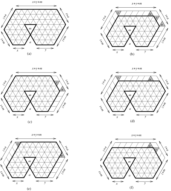
We apply Kuo Theorem 2.3 to the dual graph G๐บG of the magnet bar region Bm,aโ€‹(x,y,z,t)subscript๐ต๐‘š๐‘Ž๐‘ฅ๐‘ฆ๐‘ง๐‘กB_{m,a}(x,y,z,t) (weighted by wโ€‹t2๐‘คsubscript๐‘ก2wt_{2}). We pick the four vertices u,v,w,s๐‘ข๐‘ฃ๐‘ค๐‘ u,v,w,s as in Figure 4.3(b). In particular, the four shaded unit triangles correspond to the four vertices: the shaded unit triangle corresponding to u๐‘ขu is the lowest one, and v,w,s๐‘ฃ๐‘ค๐‘ v,w,s correspond to the next shaded unit triangles as we move counter-clockwise from the lowest one. We notice that the north side of the region has length x+y+mโ‰ฅy+mโ‰ฅ2๐‘ฅ๐‘ฆ๐‘š๐‘ฆ๐‘š2x+y+m\geq y+m\geq 2 and the northeast side has length t+aโ‰ฅ2๐‘ก๐‘Ž2t+a\geq 2, so the four vertices u,v,w,s๐‘ข๐‘ฃ๐‘ค๐‘ u,v,w,s are well-defined.

By removing the lozenges forced by the shaded unit triangles, we get back new B๐ตB-type regions weighted by wโ€‹t2๐‘คsubscript๐‘ก2wt_{2}. Collecting the weights of those forced lozenges, we get

Mโก(Gโˆ’{u,v,w,s})=q(z+m+12)+(x+y+mโˆ’2)โ€‹(z+t+m+a)โ€‹M2โก(Bm,aโ€‹(x,yโˆ’1,z,tโˆ’1)),M๐บ๐‘ข๐‘ฃ๐‘ค๐‘ superscript๐‘žbinomial๐‘ง๐‘š12๐‘ฅ๐‘ฆ๐‘š2๐‘ง๐‘ก๐‘š๐‘ŽsubscriptM2subscript๐ต๐‘š๐‘Ž๐‘ฅ๐‘ฆ1๐‘ง๐‘ก1\operatorname{M}(G-\{u,v,w,s\})=q^{\binom{z+m+1}{2}+(x+y+m-2)(z+t+m+a)}\operatorname{M}_{2}\big{(}B_{m,a}(x,y-1,z,t-1)\big{)}, (4.8)
Mโก(Gโˆ’{u,v})=q(z+m+12)โ€‹M2โก(Bm,aโ€‹(x,yโˆ’1,z,t)),M๐บ๐‘ข๐‘ฃsuperscript๐‘žbinomial๐‘ง๐‘š12subscriptM2subscript๐ต๐‘š๐‘Ž๐‘ฅ๐‘ฆ1๐‘ง๐‘ก\operatorname{M}(G-\{u,v\})=q^{\binom{z+m+1}{2}}\operatorname{M}_{2}\big{(}B_{m,a}(x,y-1,z,t)\big{)}, (4.9)
Mโก(Gโˆ’{w,s})=q(x+y+mโˆ’2)โ€‹(z+t+m+a)โ€‹M2โก(Bm,aโ€‹(x,y,z,tโˆ’1)),M๐บ๐‘ค๐‘ superscript๐‘ž๐‘ฅ๐‘ฆ๐‘š2๐‘ง๐‘ก๐‘š๐‘ŽsubscriptM2subscript๐ต๐‘š๐‘Ž๐‘ฅ๐‘ฆ๐‘ง๐‘ก1\operatorname{M}(G-\{w,s\})=q^{(x+y+m-2)(z+t+m+a)}\operatorname{M}_{2}\big{(}B_{m,a}(x,y,z,t-1)\big{)}, (4.10)
Mโก(Gโˆ’{u,s})=q(z+m+12)โ€‹M2โก(Bm,aโ€‹(x,yโˆ’1,z+1,tโˆ’1)),M๐บ๐‘ข๐‘ superscript๐‘žbinomial๐‘ง๐‘š12subscriptM2subscript๐ต๐‘š๐‘Ž๐‘ฅ๐‘ฆ1๐‘ง1๐‘ก1\operatorname{M}(G-\{u,s\})=q^{\binom{z+m+1}{2}}\operatorname{M}_{2}\big{(}B_{m,a}(x,y-1,z+1,t-1)\big{)}, (4.11)

and

Mโก(Gโˆ’{v,w})=q(x+y+mโˆ’1)โ€‹(z+t+m+a)โ€‹M2โก(Bm,aโ€‹(x,y,zโˆ’1,t))M๐บ๐‘ฃ๐‘คsuperscript๐‘ž๐‘ฅ๐‘ฆ๐‘š1๐‘ง๐‘ก๐‘š๐‘ŽsubscriptM2subscript๐ต๐‘š๐‘Ž๐‘ฅ๐‘ฆ๐‘ง1๐‘ก\operatorname{M}(G-\{v,w\})=q^{(x+y+m-1)(z+t+m+a)}\operatorname{M}_{2}\big{(}B_{m,a}(x,y,z-1,t)\big{)} (4.12)

(see Figures 4.3(b)โ€“(f), respectively). Plugging the above identities into the equation (2.1) in Kuo Condensation Theorem 2.3, we obtain

M2โก(Bm,aโ€‹(x,y,z,t))subscriptM2subscript๐ต๐‘š๐‘Ž๐‘ฅ๐‘ฆ๐‘ง๐‘ก\displaystyle\operatorname{M}_{2}\big{(}B_{m,a}(x,y,z,t)\big{)} M2โก(Bm,aโ€‹(x,yโˆ’1,z,tโˆ’1))=subscriptM2subscript๐ต๐‘š๐‘Ž๐‘ฅ๐‘ฆ1๐‘ง๐‘ก1absent\displaystyle\operatorname{M}_{2}\big{(}B_{m,a}(x,y-1,z,t-1)\big{)}=
M2โก(Bm,aโ€‹(x,yโˆ’1,z,t))โ€‹M2โก(Bm,aโ€‹(x,y,z,tโˆ’1))subscriptM2subscript๐ต๐‘š๐‘Ž๐‘ฅ๐‘ฆ1๐‘ง๐‘กsubscriptM2subscript๐ต๐‘š๐‘Ž๐‘ฅ๐‘ฆ๐‘ง๐‘ก1\displaystyle\operatorname{M}_{2}\big{(}B_{m,a}(x,y-1,z,t)\big{)}\operatorname{M}_{2}\big{(}B_{m,a}(x,y,z,t-1)\big{)}
+qz+t+m+aโ€‹M2โก(Bm,aโ€‹(x,yโˆ’1,z+1,tโˆ’1))โ€‹M2โก(Bm,aโ€‹(x,y,zโˆ’1,t)).superscript๐‘ž๐‘ง๐‘ก๐‘š๐‘ŽsubscriptM2subscript๐ต๐‘š๐‘Ž๐‘ฅ๐‘ฆ1๐‘ง1๐‘ก1subscriptM2subscript๐ต๐‘š๐‘Ž๐‘ฅ๐‘ฆ๐‘ง1๐‘ก\displaystyle+q^{z+t+m+a}\operatorname{M}_{2}\big{(}B_{m,a}(x,y-1,z+1,t-1)\big{)}\operatorname{M}_{2}\big{(}B_{m,a}(x,y,z-1,t)\big{)}. (4.13)

All regions in the above equation, except for the first one, have the sum of their y๐‘ฆy-, z๐‘งz- and t๐‘กt-parameters strictly less than y+z+t๐‘ฆ๐‘ง๐‘กy+z+t. Thus, by the induction hypothesis, those regions have their tiling generating functions given by (4.8). By substituting these formulas into the above equation and performing some simplifications, one readily gets M2โก(Bm,aโ€‹(x,y,z,t))subscriptM2subscript๐ต๐‘š๐‘Ž๐‘ฅ๐‘ฆ๐‘ง๐‘ก\operatorname{M}_{2}\left(B_{m,a}(x,y,z,t)\right) equal exactly to the expression on the right-hand side of (4.8). This finishes our proof. โˆŽ

We need another tiling q๐‘žq-enumeration of the magnet bar region as follows.

Assume that we now give all right and left lozenges in the magnet bar region Bm,aโ€‹(x,y,z,t)subscript๐ต๐‘š๐‘Ž๐‘ฅ๐‘ฆ๐‘ง๐‘กB_{m,a}(x,y,z,t) a weight 1. Next, we give a vertical lozenge a weight qlsuperscript๐‘ž๐‘™q^{l}, where l๐‘™l is the distance between the northeast side of the lozenge and the southwest side of the region. We denote by wโ€‹t3๐‘คsubscript๐‘ก3wt_{3} the new weight assignment, and M3subscriptM3\operatorname{M}_{3} the corresponding tiling generating function.

Proposition 4.9.

For non-negative integers m,a,x,y,z,t๐‘š๐‘Ž๐‘ฅ๐‘ฆ๐‘ง๐‘กm,a,x,y,z,t

M3subscriptM3\displaystyle\operatorname{M}_{3} (Bm,aโ€‹(x,y,z,t))=qmโ€‹(a+12)+tโ€‹(z+a+12)+aโ€‹(z+m)โ€‹(x+a)+aโ€‹(z+m+12)subscript๐ต๐‘š๐‘Ž๐‘ฅ๐‘ฆ๐‘ง๐‘กsuperscript๐‘ž๐‘šbinomial๐‘Ž12๐‘กbinomial๐‘ง๐‘Ž12๐‘Ž๐‘ง๐‘š๐‘ฅ๐‘Ž๐‘Žbinomial๐‘ง๐‘š12\displaystyle\big{(}B_{m,a}(x,y,z,t)\big{)}=q^{m\binom{a+1}{2}+t\binom{z+a+1}{2}+a(z+m)(x+a)+a\binom{z+m+1}{2}}
ร—Hqโก(m+a+x+y+z+t)Hqโก(m+a+x+y+t)โ€‹Hqโก(m+a+x+y+z)absentsubscriptH๐‘ž๐‘š๐‘Ž๐‘ฅ๐‘ฆ๐‘ง๐‘กsubscriptH๐‘ž๐‘š๐‘Ž๐‘ฅ๐‘ฆ๐‘กsubscriptH๐‘ž๐‘š๐‘Ž๐‘ฅ๐‘ฆ๐‘ง\displaystyle\times\frac{\operatorname{H}_{q}(m+a+x+y+z+t)}{\operatorname{H}_{q}(m+a+x+y+t)\operatorname{H}_{q}(m+a+x+y+z)}
ร—Hqโก(m+a+x+t)โ€‹Hqโก(m+a+x+y)โ€‹Hqโก(m+a+y+z)Hqโก(m+a+z+t)โ€‹Hqโก(m+a+x)โ€‹Hqโก(m+a+y)absentsubscriptH๐‘ž๐‘š๐‘Ž๐‘ฅ๐‘กsubscriptH๐‘ž๐‘š๐‘Ž๐‘ฅ๐‘ฆsubscriptH๐‘ž๐‘š๐‘Ž๐‘ฆ๐‘งsubscriptH๐‘ž๐‘š๐‘Ž๐‘ง๐‘กsubscriptH๐‘ž๐‘š๐‘Ž๐‘ฅsubscriptH๐‘ž๐‘š๐‘Ž๐‘ฆ\displaystyle\times\frac{\operatorname{H}_{q}(m+a+x+t)\operatorname{H}_{q}(m+a+x+y)\operatorname{H}_{q}(m+a+y+z)}{\operatorname{H}_{q}(m+a+z+t)\operatorname{H}_{q}(m+a+x)\operatorname{H}_{q}(m+a+y)}
ร—Hq(x)Hq(y)Hq(z)Hq(t)Hq(m)Hq(a)2Hqโก(a+x)โ€‹Hqโก(a+y)โ€‹Hqโก(z+t)โ€‹Hqโก(m+a)\displaystyle\times\frac{\operatorname{H}_{q}(x)\operatorname{H}_{q}(y)\operatorname{H}_{q}(z)\operatorname{H}_{q}(t)\operatorname{H}_{q}(m)\operatorname{H}_{q}(a)^{2}}{\operatorname{H}_{q}(a+x)\operatorname{H}_{q}(a+y)\operatorname{H}_{q}(z+t)\operatorname{H}_{q}(m+a)}
ร—Hqโก(m+z+t)โ€‹Hqโก(m+a+x)โ€‹Hqโก(m+a+y)Hqโก(m+y+z)โ€‹Hqโก(m+x+t).absentsubscriptH๐‘ž๐‘š๐‘ง๐‘กsubscriptH๐‘ž๐‘š๐‘Ž๐‘ฅsubscriptH๐‘ž๐‘š๐‘Ž๐‘ฆsubscriptH๐‘ž๐‘š๐‘ฆ๐‘งsubscriptH๐‘ž๐‘š๐‘ฅ๐‘ก\displaystyle\times\frac{\operatorname{H}_{q}(m+z+t)\operatorname{H}_{q}(m+a+x)\operatorname{H}_{q}(m+a+y)}{\operatorname{H}_{q}(m+y+z)\operatorname{H}_{q}(m+x+t)}. (4.14)
Proof.

The equality (4.9) can be treated similarly to (4.8) in the Proposition 4.8 by induction on y+z+t๐‘ฆ๐‘ง๐‘กy+z+t.

We would also like to obtain a recurrence for the M3subscriptM3\operatorname{M}_{3}-generating function of the magnet bar by using Kuo consdensation. Similar to Proposition 4.8, the application of Kuo condensation requires that the north and the northeast sides both have lengths greater than 111. Taking into account also the base cases of the recurrence, we need to verify (4.9) in the situations when a=0๐‘Ž0a=0, x=0๐‘ฅ0x=0, y=0๐‘ฆ0y=0, z=0๐‘ง0z=0 or t=0๐‘ก0t=0.

Assume that our magnet bar region is weighted by wโ€‹t3๐‘คsubscript๐‘ก3wt_{3}. We still follow the process in Figures 4.2 and 4.3, however, the reader should be aware that the weight assignment here is different from that in the proof of Proposition 4.8.

If a=0๐‘Ž0a=0, we get a weighted version of the hexagon Hโ€‹eโ€‹xโ€‹(z,x+y+m,t)๐ป๐‘’๐‘ฅ๐‘ง๐‘ฅ๐‘ฆ๐‘š๐‘กHex(z,x+y+m,t) by removing forced lozenges from the magnet bar region as in Figure 4.2(e). Rotating the hexagon 60โˆ˜superscript6060^{\circ} clockwise and reflecting the resulting region over a vertical line, we get the hexagon Hโ€‹eโ€‹xโ€‹(z,t,x+y+m)๐ป๐‘’๐‘ฅ๐‘ง๐‘ก๐‘ฅ๐‘ฆ๐‘šHex(z,t,x+y+m) weighted by wโ€‹t2๐‘คsubscript๐‘ก2wt_{2}, and (4.9) follows from Corollary 3.6.

If x=0๐‘ฅ0x=0, after removing forced vertical lozenges (whose weight product is equal to q(t+m)โ€‹(a+12)superscript๐‘ž๐‘ก๐‘šbinomial๐‘Ž12q^{(t+m)\binom{a+1}{2}}) as in Figure 4.2(a), we get a weighted region R๐‘…R. Next, we rotate R๐‘…R 60โˆ˜superscript6060^{\circ} counter-clockwise and reflect the resulting region about a vertical line. This way, we get the weighted region Kmโ€‹(a,t,z,y)subscript๐พ๐‘š๐‘Ž๐‘ก๐‘ง๐‘ฆK_{m}(a,t,z,y) in which a right lozenge is weighted by qa+lsuperscript๐‘ž๐‘Ž๐‘™q^{a+l}, where l๐‘™l is the distance from the top of the lozenge to the bottom of the region. We divide the weight of each right lozenge in the latter region by qasuperscript๐‘ž๐‘Žq^{a}, and get back the weight assignment wโ€‹t2๐‘คsubscript๐‘ก2wt_{2}. Thus,

M3โก(Bm,aโ€‹(0,y,z,t))=q(t+m)โ€‹(a+12)โ€‹qaโ€‹zโ€‹t+a2โ€‹(z+m)โ€‹M2โก(Kmโ€‹(a,t,z,y)),subscriptM3subscript๐ต๐‘š๐‘Ž0๐‘ฆ๐‘ง๐‘กsuperscript๐‘ž๐‘ก๐‘šbinomial๐‘Ž12superscript๐‘ž๐‘Ž๐‘ง๐‘กsuperscript๐‘Ž2๐‘ง๐‘šsubscriptM2subscript๐พ๐‘š๐‘Ž๐‘ก๐‘ง๐‘ฆ\operatorname{M}_{3}\big{(}B_{m,a}(0,y,z,t)\big{)}=q^{(t+m)\binom{a+1}{2}}q^{azt+a^{2}(z+m)}\operatorname{M}_{2}\big{(}K_{m}(a,t,z,y)\big{)}, (4.15)

where the factor qaโ€‹zโ€‹t+a2โ€‹(z+m)superscript๐‘ž๐‘Ž๐‘ง๐‘กsuperscript๐‘Ž2๐‘ง๐‘šq^{azt+a^{2}(z+m)} comes from the weight division. Then (4.9) follows from Lemma 3.7.

If y=0๐‘ฆ0y=0, by removing forced lozenges (whose weight product is q(x+a)โ€‹(z+m)โ€‹a+aโ€‹(z+m+12)superscript๐‘ž๐‘ฅ๐‘Ž๐‘ง๐‘š๐‘Ž๐‘Žbinomial๐‘ง๐‘š12q^{(x+a)(z+m)a+a\binom{z+m+1}{2}}) and rotating the resulting region 60โˆ˜superscript6060^{\circ} clockwise, we get a weighted version of region Kmโ€‹(a,z,t,x)subscript๐พ๐‘š๐‘Ž๐‘ง๐‘ก๐‘ฅK_{m}(a,z,t,x) in which a right lozenge is weighted by qm+a+x+z+1โˆ’lsuperscript๐‘ž๐‘š๐‘Ž๐‘ฅ๐‘ง1๐‘™q^{m+a+x+z+1-l}, where l๐‘™l is the distance from the left side of the lozenge and the southeast side of the region (see Figure 4.2(b)). By dividing the weight of each right lozenge by qm+a+x+z+1superscript๐‘ž๐‘š๐‘Ž๐‘ฅ๐‘ง1q^{m+a+x+z+1}, we get back the weight assignment wโ€‹t1๐‘คsubscript๐‘ก1wt_{1}, where q๐‘žq is replaced by qโˆ’1superscript๐‘ž1q^{-1}. Thus, (4.9) follows from Proposition 3.5, Lemma 3.7 and the simple fact [n]qโˆ’1=[n]q/qnโˆ’1subscriptdelimited-[]๐‘›superscript๐‘ž1subscriptdelimited-[]๐‘›๐‘žsuperscript๐‘ž๐‘›1[n]_{q^{-1}}=[n]_{q}/q^{n-1}.

If z=0๐‘ง0z=0, we apply Region-splitting Lemma 2.4 (and remove forced lozenges weighted by 111) to split our region into two hexagons as in Figure 4.2(c). Next, we rotate the right hexagon 60โˆ˜superscript6060^{\circ} counter-clockwise and reflect the resulting hexagon about a vertical line to get the hexagon Hโ€‹eโ€‹xโ€‹(a,t+m,x)๐ป๐‘’๐‘ฅ๐‘Ž๐‘ก๐‘š๐‘ฅHex(a,t+m,x) weighted by wโ€‹t2๐‘คsubscript๐‘ก2wt_{2}. For the left hexagon, we also rotate it 60โˆ˜superscript6060^{\circ} counter-clockwise, reflect the resulting region about a vertical line and divide the weight of each right lozenge of it by qx+asuperscript๐‘ž๐‘ฅ๐‘Žq^{x+a} to get the hexagon Hโ€‹eโ€‹xโ€‹(m,a,y)๐ป๐‘’๐‘ฅ๐‘š๐‘Ž๐‘ฆHex(m,a,y) weighted by wโ€‹t2๐‘คsubscript๐‘ก2wt_{2}. Then we get (4.9) from Corollary 3.6. The case when t=0๐‘ก0t=0, can be treated similarly to the case when z=0๐‘ง0z=0, based on Figure 4.2(d).

The induction step is completely analogous to that of the proof of Proposition 4.8. We also apply Kuoโ€™s Theorem 2.3, based on Figure 4.3. The vertices u,v,w,s๐‘ข๐‘ฃ๐‘ค๐‘ u,v,w,s are well-defined because the north side of the magnet bar has length x+y+mโ‰ฅx+yโ‰ฅ2๐‘ฅ๐‘ฆ๐‘š๐‘ฅ๐‘ฆ2x+y+m\geq x+y\geq 2 and the northeast side has length t+aโ‰ฅ2๐‘ก๐‘Ž2t+a\geq 2. After removing lozenges forced by the shaded unit triangles, we get back new B๐ตB-type regions weighted by wโ€‹t3๐‘คsubscript๐‘ก3wt_{3}. Figure 4.3 tells us that the product of M3subscriptM3\operatorname{M}_{3}-generating functions of the two regions on the top is equal to the product of the M3subscriptM3\operatorname{M}_{3}-generating functions of the two regions in the middle plus the product of M3subscriptM3\operatorname{M}_{3}-generating functions of the two regions on the bottom. To be precise, we get the following recurrence

M3(Bm,a(x,y,z,t)\displaystyle\operatorname{M}_{3}\big{(}B_{m,a}(x,y,z,t) )M3(Bm,a(x,yโˆ’1,z,tโˆ’1))=\displaystyle\big{)}\operatorname{M}_{3}\big{(}B_{m,a}(x,y-1,z,t-1)\big{)}=
M3โก(Bm,aโ€‹(x,yโˆ’1,z,t))โ€‹M3โก(Bm,aโ€‹(x,y,z,tโˆ’1))subscriptM3subscript๐ต๐‘š๐‘Ž๐‘ฅ๐‘ฆ1๐‘ง๐‘กsubscriptM3subscript๐ต๐‘š๐‘Ž๐‘ฅ๐‘ฆ๐‘ง๐‘ก1\displaystyle\operatorname{M}_{3}\big{(}B_{m,a}(x,y-1,z,t)\big{)}\operatorname{M}_{3}\big{(}B_{m,a}(x,y,z,t-1)\big{)}
+qm+a+x+y+zโ€‹M3โก(Bm,aโ€‹(x,yโˆ’1,z+1,tโˆ’1))โ€‹M3โก(Bm,aโ€‹(x,y,zโˆ’1,t)),superscript๐‘ž๐‘š๐‘Ž๐‘ฅ๐‘ฆ๐‘งsubscriptM3subscript๐ต๐‘š๐‘Ž๐‘ฅ๐‘ฆ1๐‘ง1๐‘ก1subscriptM3subscript๐ต๐‘š๐‘Ž๐‘ฅ๐‘ฆ๐‘ง1๐‘ก\displaystyle+q^{m+a+x+y+z}\operatorname{M}_{3}\big{(}B_{m,a}(x,y-1,z+1,t-1)\big{)}\operatorname{M}_{3}\big{(}B_{m,a}(x,y,z-1,t)\big{)}, (4.16)

and the proposition follows from the induction hypothesis. โˆŽ

Remark 1.

In some sense, Proposition 4.9 is equivalent to Proposition 4.8 in the same way as the three weightings in Proposition 3.5 are equivalent. Indeed, we first introduce an analog wโ€‹tโ€ฒ๐‘คsuperscript๐‘กโ€ฒwt^{\prime} of the natural weight assignment wโ€‹t0๐‘คsubscript๐‘ก0wt_{0}, by viewing each vertical lozenge in a tiling T๐‘‡T as the right face of a horizontal block running from left to right in the pile ฯ€Tsubscript๐œ‹๐‘‡\pi_{T} corresponding to T๐‘‡T. Each vertical lozenge is now weighted by qxsuperscript๐‘ž๐‘ฅq^{x}, where x๐‘ฅx is the length of its corresponding block. Using the same arguments as used when comparing wโ€‹t2๐‘คsubscript๐‘ก2wt_{2} and wโ€‹t0๐‘คsubscript๐‘ก0wt_{0} in Proposition 3.5, one can show that wโ€‹t3๐‘คsubscript๐‘ก3wt_{3} and wโ€‹tโ€ฒ๐‘คsuperscript๐‘กโ€ฒwt^{\prime} are only different by some power of q๐‘žq. Moreover, we note that wโ€‹tโ€ฒโ€‹(T)=wโ€‹t0โ€‹(T)=q|ฯ€T|๐‘คsuperscript๐‘กโ€ฒ๐‘‡๐‘คsubscript๐‘ก0๐‘‡superscript๐‘žsubscript๐œ‹๐‘‡wt^{\prime}(T)=wt_{0}(T)=q^{|\pi_{T}|}, for any tiling T๐‘‡T of the region. This implies that wโ€‹t2๐‘คsubscript๐‘ก2wt_{2} and wโ€‹t3๐‘คsubscript๐‘ก3wt_{3} are only different by some multiplicative factor, and Proposition 4.9 follows from Proposition 4.8 (and vice versa).

5 Proof of Theorem 1.2

By Proposition 3.5, we only need to show that

M2subscriptM2\displaystyle\operatorname{M}_{2} (Qโ€‹(xyztmabc))=๐‘„matrix๐‘ฅ๐‘ฆ๐‘ง๐‘ก๐‘š๐‘Ž๐‘๐‘absent\displaystyle\left(Q\begin{pmatrix}x&y&z&t\\ m&a&b&c\end{pmatrix}\right)=
qgโ€‹(xyztmabc)โ€‹Hqโก(m+a+b+c+x+y+z+t)Hqโก(m+a+b+c+x+y+t)โ€‹Hqโก(m+a+b+c+x+y+z)superscript๐‘žgmatrix๐‘ฅ๐‘ฆ๐‘ง๐‘ก๐‘š๐‘Ž๐‘๐‘subscriptH๐‘ž๐‘š๐‘Ž๐‘๐‘๐‘ฅ๐‘ฆ๐‘ง๐‘กsubscriptH๐‘ž๐‘š๐‘Ž๐‘๐‘๐‘ฅ๐‘ฆ๐‘กsubscriptH๐‘ž๐‘š๐‘Ž๐‘๐‘๐‘ฅ๐‘ฆ๐‘ง\displaystyle q^{\textbf{g}\begin{pmatrix}x&y&z&t\\ m&a&b&c\end{pmatrix}}\frac{\operatorname{H}_{q}(m+a+b+c+x+y+z+t)}{\operatorname{H}_{q}(m+a+b+c+x+y+t)\operatorname{H}_{q}(m+a+b+c+x+y+z)}
ร—Hqโก(m+a+b+c+x+t)โ€‹Hqโก(m+a+b+c+x+y)โ€‹Hqโก(m+a+b+c+y+z)Hqโก(m+a+b+c+z+t)โ€‹Hqโก(m+a+b+c+x)โ€‹Hqโก(m+a+b+c+y)absentsubscriptH๐‘ž๐‘š๐‘Ž๐‘๐‘๐‘ฅ๐‘กsubscriptH๐‘ž๐‘š๐‘Ž๐‘๐‘๐‘ฅ๐‘ฆsubscriptH๐‘ž๐‘š๐‘Ž๐‘๐‘๐‘ฆ๐‘งsubscriptH๐‘ž๐‘š๐‘Ž๐‘๐‘๐‘ง๐‘กsubscriptH๐‘ž๐‘š๐‘Ž๐‘๐‘๐‘ฅsubscriptH๐‘ž๐‘š๐‘Ž๐‘๐‘๐‘ฆ\displaystyle\times\frac{\operatorname{H}_{q}(m+a+b+c+x+t)\operatorname{H}_{q}(m+a+b+c+x+y)\operatorname{H}_{q}(m+a+b+c+y+z)}{\operatorname{H}_{q}(m+a+b+c+z+t)\operatorname{H}_{q}(m+a+b+c+x)\operatorname{H}_{q}(m+a+b+c+y)}
ร—Hqโก(x)โ€‹Hqโก(y)โ€‹Hqโก(z)โ€‹Hqโก(t)Hqโก(x+t)โ€‹Hqโก(y+z)โ€‹Hq(m)3Hq(a)2Hq(b)Hq(c)Hq(m+a+b+c)Hq(m+a)2Hq(m+b)Hq(m+c)\displaystyle\times\frac{\operatorname{H}_{q}(x)\operatorname{H}_{q}(y)\operatorname{H}_{q}(z)\operatorname{H}_{q}(t)}{\operatorname{H}_{q}(x+t)\operatorname{H}_{q}(y+z)}\frac{\operatorname{H}_{q}(m)^{3}\operatorname{H}_{q}(a)^{2}\operatorname{H}_{q}(b)\operatorname{H}_{q}(c)\operatorname{H}_{q}(m+a+b+c)}{\operatorname{H}_{q}(m+a)^{2}\operatorname{H}_{q}(m+b)\operatorname{H}_{q}(m+c)}
ร—Hqโก(m+b+c+z+t)โ€‹Hqโก(m+a+c+x)โ€‹Hqโก(m+a+b+y)Hqโก(m+b+y+z)โ€‹Hqโก(m+c+x+t)absentsubscriptH๐‘ž๐‘š๐‘๐‘๐‘ง๐‘กsubscriptH๐‘ž๐‘š๐‘Ž๐‘๐‘ฅsubscriptH๐‘ž๐‘š๐‘Ž๐‘๐‘ฆsubscriptH๐‘ž๐‘š๐‘๐‘ฆ๐‘งsubscriptH๐‘ž๐‘š๐‘๐‘ฅ๐‘ก\displaystyle\times\frac{\operatorname{H}_{q}(m+b+c+z+t)\operatorname{H}_{q}(m+a+c+x)\operatorname{H}_{q}(m+a+b+y)}{\operatorname{H}_{q}(m+b+y+z)\operatorname{H}_{q}(m+c+x+t)}
ร—Hqโก(c+x+t)โ€‹Hqโก(b+y+z)Hqโก(a+c+x)โ€‹Hqโก(a+b+y)โ€‹Hqโก(b+c+z+t).absentsubscriptH๐‘ž๐‘๐‘ฅ๐‘กsubscriptH๐‘ž๐‘๐‘ฆ๐‘งsubscriptH๐‘ž๐‘Ž๐‘๐‘ฅsubscriptH๐‘ž๐‘Ž๐‘๐‘ฆsubscriptH๐‘ž๐‘๐‘๐‘ง๐‘ก\displaystyle\times\frac{\operatorname{H}_{q}(c+x+t)\operatorname{H}_{q}(b+y+z)}{\operatorname{H}_{q}(a+c+x)\operatorname{H}_{q}(a+b+y)\operatorname{H}_{q}(b+c+z+t)}. (5.1)
Refer to caption
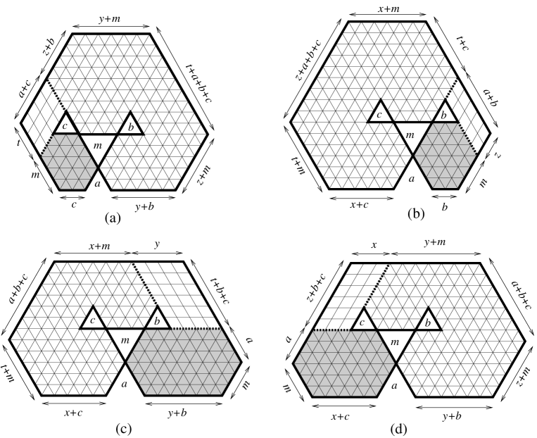
Figure 5.1: The four base cases: (a) x=0๐‘ฅ0x=0, (b) y=0๐‘ฆ0y=0, (c) z=0๐‘ง0z=0 (b), and t=0๐‘ก0t=0.

We prove (5) by induction on y+z+t๐‘ฆ๐‘ง๐‘กy+z+t. We assume that our region Q:=Qโ€‹(xyztmabc)assign๐‘„๐‘„matrix๐‘ฅ๐‘ฆ๐‘ง๐‘ก๐‘š๐‘Ž๐‘๐‘Q:=Q\begin{pmatrix}x&y&z&t\\ m&a&b&c\end{pmatrix} is weighted by wโ€‹t2๐‘คsubscript๐‘ก2wt_{2}

Similarly to the case of the magnet bars in Propositions 4.8 and 4.9, we will use Kuoโ€™s condensation Theorem 2.3 to obtain a recurrence for the M2subscriptM2\operatorname{M}_{2}-generating function of the Q๐‘„Q-type region. In order to apply the theorem, certain side-lengths of the region Q๐‘„Q must be large enough. In particular, this requires x+y+mโ‰ฅ2๐‘ฅ๐‘ฆ๐‘š2x+y+m\geq 2 and t+a+b+cโ‰ฅ2๐‘ก๐‘Ž๐‘๐‘2t+a+b+c\geq 2. Taking into account also the base cases of the recurrence, we need to verify (5) in the cases when one of the four parameters x,y,z,t๐‘ฅ๐‘ฆ๐‘ง๐‘กx,y,z,t equals 00.

If x=0๐‘ฅ0x=0, by applying Region-splitting Lemma 2.4, we split Q๐‘„Q into two parts as in Figure 5.1(a): the shaded hexagon Hโ€‹eโ€‹xโ€‹(a,c,m)๐ป๐‘’๐‘ฅ๐‘Ž๐‘๐‘šHex(a,c,m) (weighted by wโ€‹t2๐‘คsubscript๐‘ก2wt_{2}) and Qโˆ’Hโ€‹eโ€‹xโ€‹(a,c,m)๐‘„๐ป๐‘’๐‘ฅ๐‘Ž๐‘๐‘šQ-Hex(a,c,m). After removing forced vertical lozenges (which have the weight 1) from the latter region, we get a weighted magnet bar region (rotated 60โˆ˜superscript6060^{\circ}). Rotating the magnet bar region 60โˆ˜superscript6060^{\circ} counter-clockwise and reflecting the resulting region about a vertical line, we get the magnet bar region Bb,mโ€‹(a,t+c,z,y)subscript๐ต๐‘๐‘š๐‘Ž๐‘ก๐‘๐‘ง๐‘ฆB_{b,m}(a,t+c,z,y) weighted by wโ€‹t3๐‘คsubscript๐‘ก3wt_{3}. Thus, we have

M2โก(Qโ€‹(0yztmabc))subscriptM2๐‘„matrix0๐‘ฆ๐‘ง๐‘ก๐‘š๐‘Ž๐‘๐‘\displaystyle\operatorname{M}_{2}\left(Q\begin{pmatrix}0&y&z&t\\ m&a&b&c\end{pmatrix}\right) =M2โก(Hโ€‹eโ€‹xโ€‹(a,c,m))โ€‹M3โก(Qโ€‹(0yztmabc)โˆ’Hโ€‹eโ€‹xโ€‹(a,c,m))absentsubscriptM2๐ป๐‘’๐‘ฅ๐‘Ž๐‘๐‘šsubscriptM3๐‘„matrix0๐‘ฆ๐‘ง๐‘ก๐‘š๐‘Ž๐‘๐‘๐ป๐‘’๐‘ฅ๐‘Ž๐‘๐‘š\displaystyle=\operatorname{M}_{2}\big{(}Hex(a,c,m)\big{)}\operatorname{M}_{3}\left(Q\begin{pmatrix}0&y&z&t\\ m&a&b&c\end{pmatrix}-Hex(a,c,m)\right)
=M2โก(Hโ€‹eโ€‹xโ€‹(a,c,m))โ€‹M3โก(Bb,mโ€‹(a,t+c,z,y)),absentsubscriptM2๐ป๐‘’๐‘ฅ๐‘Ž๐‘๐‘šsubscriptM3subscript๐ต๐‘๐‘š๐‘Ž๐‘ก๐‘๐‘ง๐‘ฆ\displaystyle=\operatorname{M}_{2}\big{(}Hex(a,c,m)\big{)}\operatorname{M}_{3}\big{(}B_{b,m}(a,t+c,z,y)\big{)}, (5.2)

and (5) follows from Corollary 3.6 and Proposition 4.9. The case t=0๐‘ก0t=0 can be treated similarly to the case x=0๐‘ฅ0x=0, based on Figure 5.1(d). The only difference is that our forced right lozenges have weight product equal to qxโ€‹(a+m)โ€‹(z+b+c)+xโ€‹(z+b+c+12)superscript๐‘ž๐‘ฅ๐‘Ž๐‘š๐‘ง๐‘๐‘๐‘ฅbinomial๐‘ง๐‘๐‘12q^{x(a+m)(z+b+c)+x\binom{z+b+c+1}{2}}. Thus, we get

M2subscriptM2\displaystyle\operatorname{M}_{2} (Qโ€‹(xyz0mabc))๐‘„matrix๐‘ฅ๐‘ฆ๐‘ง0๐‘š๐‘Ž๐‘๐‘\displaystyle\left(Q\begin{pmatrix}x&y&z&0\\ m&a&b&c\end{pmatrix}\right)
=M2โก(Hโ€‹eโ€‹xโ€‹(a,x+c,m))โ€‹M2โก(Qโ€‹(xyz0mabc)โˆ’Hโ€‹eโ€‹xโ€‹(a,x+c,m))absentsubscriptM2๐ป๐‘’๐‘ฅ๐‘Ž๐‘ฅ๐‘๐‘šsubscriptM2๐‘„matrix๐‘ฅ๐‘ฆ๐‘ง0๐‘š๐‘Ž๐‘๐‘๐ป๐‘’๐‘ฅ๐‘Ž๐‘ฅ๐‘๐‘š\displaystyle=\operatorname{M}_{2}\big{(}Hex(a,x+c,m)\big{)}\operatorname{M}_{2}\left(Q\begin{pmatrix}x&y&z&0\\ m&a&b&c\end{pmatrix}-Hex(a,x+c,m)\right)
=M2โก(Hโ€‹eโ€‹xโ€‹(a,x+c,m))โ€‹qxโ€‹(a+m)โ€‹(z+b+c)+xโ€‹(z+b+c+12)โ€‹M3โก(Bb,mโ€‹(a,c,z,y)).absentsubscriptM2๐ป๐‘’๐‘ฅ๐‘Ž๐‘ฅ๐‘๐‘šsuperscript๐‘ž๐‘ฅ๐‘Ž๐‘š๐‘ง๐‘๐‘๐‘ฅbinomial๐‘ง๐‘๐‘12subscriptM3subscript๐ต๐‘๐‘š๐‘Ž๐‘๐‘ง๐‘ฆ\displaystyle=\operatorname{M}_{2}\big{(}Hex(a,x+c,m)\big{)}q^{x(a+m)(z+b+c)+x\binom{z+b+c+1}{2}}\operatorname{M}_{3}\big{(}B_{b,m}(a,c,z,y)\big{)}. (5.3)

Again, (5) follows from Corollary 3.6 and Proposition 4.9.

If y=0๐‘ฆ0y=0, by Region-splitting Lemma 2.4, we get

M2โก(Qโ€‹(x0ztmabc))=M2โก(Hโ€‹eโ€‹xโ€‹(m,b,a))โ€‹M2โก(Qโ€‹(x0ztmabc)โˆ’Hโ€‹eโ€‹xโ€‹(m,b,a))subscriptM2๐‘„matrix๐‘ฅ0๐‘ง๐‘ก๐‘š๐‘Ž๐‘๐‘subscriptM2๐ป๐‘’๐‘ฅ๐‘š๐‘๐‘ŽsubscriptM2๐‘„matrix๐‘ฅ0๐‘ง๐‘ก๐‘š๐‘Ž๐‘๐‘๐ป๐‘’๐‘ฅ๐‘š๐‘๐‘Ž\operatorname{M}_{2}\left(Q\begin{pmatrix}x&0&z&t\\ m&a&b&c\end{pmatrix}\right)=\operatorname{M}_{2}\big{(}Hex(m,b,a)\big{)}\operatorname{M}_{2}\left(Q\begin{pmatrix}x&0&z&t\\ m&a&b&c\end{pmatrix}-Hex(m,b,a)\right) (5.4)

(see Figure 5.1(b)). We also remove forced lozenges (having weight 1) from the second region on the right-hand side to get a region Rโ€ฒsuperscript๐‘…โ€ฒR^{\prime}. Next, we rotate Rโ€ฒsuperscript๐‘…โ€ฒR^{\prime} 60โˆ˜superscript6060^{\circ} clockwise and reflect it about a vertical line to get the magnet bar Bc,mโ€‹(b+z,a,x,t)subscript๐ต๐‘๐‘š๐‘๐‘ง๐‘Ž๐‘ฅ๐‘กB_{c,m}(b+z,a,x,t) weighted by wโ€‹t1๐‘คsubscript๐‘ก1wt_{1}. Thus, we have

M2โก(Qโ€‹(x0ztmabc))=M2โก(Hโ€‹eโ€‹xโ€‹(m,b,a))โ€‹M1โก(Bc,mโ€‹(b+z,a,x,t)),subscriptM2๐‘„matrix๐‘ฅ0๐‘ง๐‘ก๐‘š๐‘Ž๐‘๐‘subscriptM2๐ป๐‘’๐‘ฅ๐‘š๐‘๐‘ŽsubscriptM1subscript๐ต๐‘๐‘š๐‘๐‘ง๐‘Ž๐‘ฅ๐‘ก\operatorname{M}_{2}\left(Q\begin{pmatrix}x&0&z&t\\ m&a&b&c\end{pmatrix}\right)=\operatorname{M}_{2}\big{(}Hex(m,b,a)\big{)}\operatorname{M}_{1}\big{(}B_{c,m}(b+z,a,x,t)\big{)}, (5.5)

and (5) follows from Corollary 3.6 and Propositions 3.5 and 4.8. The case z=0๐‘ง0z=0 can be obtained in the same way, based on Figure 5.1(c).
Refer to caption
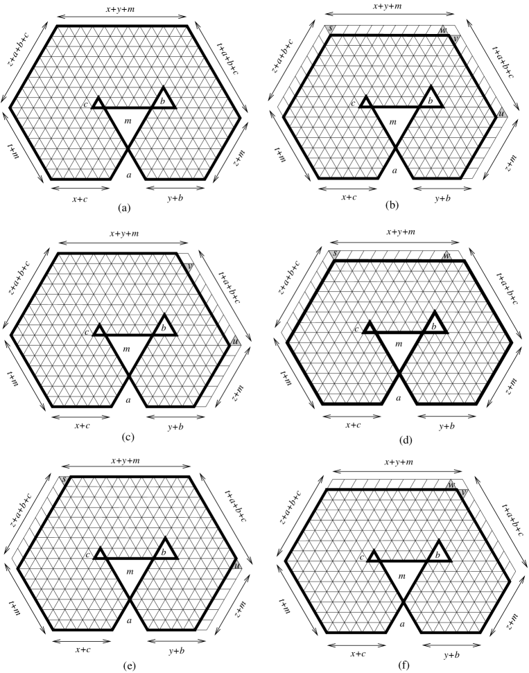
Figure 5.2: Obtaining the recurrence on the numbers of tilings by using Kuoโ€™s condensation.

For the induction step, we assume that x,y,z,t๐‘ฅ๐‘ฆ๐‘ง๐‘กx,y,z,t are positive and that (5) holds for any Q๐‘„Q-type regions in which the sum of the y๐‘ฆy-, z๐‘งz- and t๐‘กt-parameters is strictly less than y+z+t๐‘ฆ๐‘ง๐‘กy+z+t.

If b=c=0๐‘๐‘0b=c=0, then (5) follows directly from Proposition 4.8. Therefore, we can assume, from now on, that b+cโ‰ฅ1๐‘๐‘1b+c\geq 1.

We now apply Kuo condensation to the dual graph G๐บG of the region Qโ€‹(xyztmabc)๐‘„matrix๐‘ฅ๐‘ฆ๐‘ง๐‘ก๐‘š๐‘Ž๐‘๐‘Q\begin{pmatrix}x&y&z&t\\ m&a&b&c\end{pmatrix} weighted by wโ€‹t2๐‘คsubscript๐‘ก2wt_{2}. The four vertices u,v,w,s๐‘ข๐‘ฃ๐‘ค๐‘ u,v,w,s correspond to the four shaded unit triangles in Figure 5.2(b). We notice that the north side of the region has length x+y+mโ‰ฅx+yโ‰ฅ2๐‘ฅ๐‘ฆ๐‘š๐‘ฅ๐‘ฆ2x+y+m\geq x+y\geq 2 and the northeast side has length t+a+b+cโ‰ฅt+b+cโ‰ฅ2๐‘ก๐‘Ž๐‘๐‘๐‘ก๐‘๐‘2t+a+b+c\geq t+b+c\geq 2, so the four vertices u,,v,w,su,,v,w,s are well-defined. By collecting the weights of the forced lozenges shown in Figures 5.2(b)โ€“(f), we get respectively

Mโก(Gโˆ’{u,v,w,s})=q(z+m+12)+(x+y+mโˆ’2)โ€‹(z+t+m+a+b+c)โ€‹M2โก(Qโ€‹(xyโˆ’1ztโˆ’1mabc)),M๐บ๐‘ข๐‘ฃ๐‘ค๐‘ superscript๐‘žbinomial๐‘ง๐‘š12๐‘ฅ๐‘ฆ๐‘š2๐‘ง๐‘ก๐‘š๐‘Ž๐‘๐‘subscriptM2๐‘„matrix๐‘ฅ๐‘ฆ1๐‘ง๐‘ก1๐‘š๐‘Ž๐‘๐‘\operatorname{M}(G-\{u,v,w,s\})=q^{\binom{z+m+1}{2}+(x+y+m-2)(z+t+m+a+b+c)}\operatorname{M}_{2}\left(Q\begin{pmatrix}x&y-1&z&t-1\\ m&a&b&c\end{pmatrix}\right), (5.6)
Mโก(Gโˆ’{u,v})=q(z+m+12)โ€‹M2โก(Qโ€‹(xyโˆ’1ztmabc)),M๐บ๐‘ข๐‘ฃsuperscript๐‘žbinomial๐‘ง๐‘š12subscriptM2๐‘„matrix๐‘ฅ๐‘ฆ1๐‘ง๐‘ก๐‘š๐‘Ž๐‘๐‘\operatorname{M}(G-\{u,v\})=q^{\binom{z+m+1}{2}}\operatorname{M}_{2}\left(Q\begin{pmatrix}x&y-1&z&t\\ m&a&b&c\end{pmatrix}\right), (5.7)
Mโก(Gโˆ’{w,s})=q(x+y+mโˆ’2)โ€‹(z+t+m+a+b+c)โ€‹M2โก(Qโ€‹(xyztโˆ’1mabc)),M๐บ๐‘ค๐‘ superscript๐‘ž๐‘ฅ๐‘ฆ๐‘š2๐‘ง๐‘ก๐‘š๐‘Ž๐‘๐‘subscriptM2๐‘„matrix๐‘ฅ๐‘ฆ๐‘ง๐‘ก1๐‘š๐‘Ž๐‘๐‘\operatorname{M}(G-\{w,s\})=q^{(x+y+m-2)(z+t+m+a+b+c)}\operatorname{M}_{2}\left(Q\begin{pmatrix}x&y&z&t-1\\ m&a&b&c\end{pmatrix}\right), (5.8)
Mโก(Gโˆ’{u,s})=q(z+m+12)โ€‹M2โก(Qโ€‹(xyโˆ’1z+1tโˆ’1mabc)),M๐บ๐‘ข๐‘ superscript๐‘žbinomial๐‘ง๐‘š12subscriptM2๐‘„matrix๐‘ฅ๐‘ฆ1๐‘ง1๐‘ก1๐‘š๐‘Ž๐‘๐‘\operatorname{M}(G-\{u,s\})=q^{\binom{z+m+1}{2}}\operatorname{M}_{2}\left(Q\begin{pmatrix}x&y-1&z+1&t-1\\ m&a&b&c\end{pmatrix}\right), (5.9)

and

Mโก(Gโˆ’{v,w})=q(x+y+mโˆ’1)โ€‹(z+t+m+a+b+c)โ€‹M2โก(Qโ€‹(xyzโˆ’1tmabc)).M๐บ๐‘ฃ๐‘คsuperscript๐‘ž๐‘ฅ๐‘ฆ๐‘š1๐‘ง๐‘ก๐‘š๐‘Ž๐‘๐‘subscriptM2๐‘„matrix๐‘ฅ๐‘ฆ๐‘ง1๐‘ก๐‘š๐‘Ž๐‘๐‘\operatorname{M}(G-\{v,w\})=q^{(x+y+m-1)(z+t+m+a+b+c)}\operatorname{M}_{2}\left(Q\begin{pmatrix}x&y&z-1&t\\ m&a&b&c\end{pmatrix}\right). (5.10)

Substituting (5.6)โ€“(5.10) into equation (2.1) in Kuoโ€™s Theorem 2.3, we get

M2subscriptM2\displaystyle\operatorname{M}_{2} (Qโ€‹(xyztmabc))โ€‹M2โก(Qโ€‹(xyโˆ’1ztโˆ’1mabc))๐‘„matrix๐‘ฅ๐‘ฆ๐‘ง๐‘ก๐‘š๐‘Ž๐‘๐‘subscriptM2๐‘„matrix๐‘ฅ๐‘ฆ1๐‘ง๐‘ก1๐‘š๐‘Ž๐‘๐‘\displaystyle\left(Q\begin{pmatrix}x&y&z&t\\ m&a&b&c\end{pmatrix}\right)\operatorname{M}_{2}\left(Q\begin{pmatrix}x&y-1&z&t-1\\ m&a&b&c\end{pmatrix}\right)
=M2โก(Qโ€‹(xyโˆ’1ztmabc))โ€‹M2โก(Qโ€‹(xyztโˆ’1mabc))absentsubscriptM2๐‘„matrix๐‘ฅ๐‘ฆ1๐‘ง๐‘ก๐‘š๐‘Ž๐‘๐‘subscriptM2๐‘„matrix๐‘ฅ๐‘ฆ๐‘ง๐‘ก1๐‘š๐‘Ž๐‘๐‘\displaystyle=\operatorname{M}_{2}\left(Q\begin{pmatrix}x&y-1&z&t\\ m&a&b&c\end{pmatrix}\right)\operatorname{M}_{2}\left(Q\begin{pmatrix}x&y&z&t-1\\ m&a&b&c\end{pmatrix}\right)
+qz+t+m+a+b+cโ€‹M2โก(Qโ€‹(xyโˆ’1z+1tโˆ’1mabc))โ€‹M2โก(Qโ€‹(xyzโˆ’1tmabc)).superscript๐‘ž๐‘ง๐‘ก๐‘š๐‘Ž๐‘๐‘subscriptM2๐‘„matrix๐‘ฅ๐‘ฆ1๐‘ง1๐‘ก1๐‘š๐‘Ž๐‘๐‘subscriptM2๐‘„matrix๐‘ฅ๐‘ฆ๐‘ง1๐‘ก๐‘š๐‘Ž๐‘๐‘\displaystyle+q^{z+t+m+a+b+c}\operatorname{M}_{2}\left(Q\begin{pmatrix}x&y-1&z+1&t-1\\ m&a&b&c\end{pmatrix}\right)\operatorname{M}_{2}\left(Q\begin{pmatrix}x&y&z-1&t\\ m&a&b&c\end{pmatrix}\right). (5.11)

Finally, if we denote by ฮจโ€‹(xyztmabc)ฮจmatrix๐‘ฅ๐‘ฆ๐‘ง๐‘ก๐‘š๐‘Ž๐‘๐‘\Psi\begin{pmatrix}x&y&z&t\\ m&a&b&c\end{pmatrix} the expression on the right-hand side of (5), we only need to show that ฮจฮจ\Psi also satisfies the recurrence (5). Equivalently, we need to verify that

ฮจโ€‹(xyโˆ’1ztmabc)ฮจโ€‹(xyztmabc)ฮจmatrix๐‘ฅ๐‘ฆ1๐‘ง๐‘ก๐‘š๐‘Ž๐‘๐‘ฮจmatrix๐‘ฅ๐‘ฆ๐‘ง๐‘ก๐‘š๐‘Ž๐‘๐‘\displaystyle\frac{\Psi\begin{pmatrix}x&y-1&z&t\\ m&a&b&c\end{pmatrix}}{\Psi\begin{pmatrix}x&y&z&t\\ m&a&b&c\end{pmatrix}} ฮจโ€‹(xyztโˆ’1mabc)ฮจโ€‹(xyโˆ’1ztโˆ’1mabc)+limit-fromฮจmatrix๐‘ฅ๐‘ฆ๐‘ง๐‘ก1๐‘š๐‘Ž๐‘๐‘ฮจmatrix๐‘ฅ๐‘ฆ1๐‘ง๐‘ก1๐‘š๐‘Ž๐‘๐‘\displaystyle\frac{\Psi\begin{pmatrix}x&y&z&t-1\\ m&a&b&c\end{pmatrix}}{\Psi\begin{pmatrix}x&y-1&z&t-1\\ m&a&b&c\end{pmatrix}}+
qz+t+m+a+b+cโ€‹ฮจโ€‹(xyzโˆ’1tmabc)ฮจโ€‹(xyztmabc)โ€‹ฮจโ€‹(xyโˆ’1z+1tโˆ’1mabc)ฮจโ€‹(xyโˆ’1ztโˆ’1mabc)=1.superscript๐‘ž๐‘ง๐‘ก๐‘š๐‘Ž๐‘๐‘ฮจmatrix๐‘ฅ๐‘ฆ๐‘ง1๐‘ก๐‘š๐‘Ž๐‘๐‘ฮจmatrix๐‘ฅ๐‘ฆ๐‘ง๐‘ก๐‘š๐‘Ž๐‘๐‘ฮจmatrix๐‘ฅ๐‘ฆ1๐‘ง1๐‘ก1๐‘š๐‘Ž๐‘๐‘ฮจmatrix๐‘ฅ๐‘ฆ1๐‘ง๐‘ก1๐‘š๐‘Ž๐‘๐‘1\displaystyle q^{z+t+m+a+b+c}\frac{\Psi\begin{pmatrix}x&y&z-1&t\\ m&a&b&c\end{pmatrix}}{\Psi\begin{pmatrix}x&y&z&t\\ m&a&b&c\end{pmatrix}}\frac{\Psi\begin{pmatrix}x&y-1&z+1&t-1\\ m&a&b&c\end{pmatrix}}{\Psi\begin{pmatrix}x&y-1&z&t-1\\ m&a&b&c\end{pmatrix}}=1. (5.12)

Let ฮฆโ€‹(xyztmabc):=qโˆ’gโ€‹(xyztmabc)โ€‹ฮจโ€‹(xyztmabc)assignฮฆmatrix๐‘ฅ๐‘ฆ๐‘ง๐‘ก๐‘š๐‘Ž๐‘๐‘superscript๐‘žgmatrix๐‘ฅ๐‘ฆ๐‘ง๐‘ก๐‘š๐‘Ž๐‘๐‘ฮจmatrix๐‘ฅ๐‘ฆ๐‘ง๐‘ก๐‘š๐‘Ž๐‘๐‘\Phi\begin{pmatrix}x&y&z&t\\ m&a&b&c\end{pmatrix}:=q^{-\textbf{g}\begin{pmatrix}x&y&z&t\\ m&a&b&c\end{pmatrix}}\Psi\begin{pmatrix}x&y&z&t\\ m&a&b&c\end{pmatrix}. We notice that the function ฮฆโ€‹(xyztmabc)ฮฆmatrix๐‘ฅ๐‘ฆ๐‘ง๐‘ก๐‘š๐‘Ž๐‘๐‘\Phi\begin{pmatrix}x&y&z&t\\ m&a&b&c\end{pmatrix} is simply the expression on the right-hand side of (1.2). By the definition of the function g, we get

gโ€‹(xyโˆ’1ztmabc)+gโ€‹(xyztโˆ’1mabc)=gโ€‹(xyztmabc)+gโ€‹(xyโˆ’1ztโˆ’1mabc)gmatrix๐‘ฅ๐‘ฆ1๐‘ง๐‘ก๐‘š๐‘Ž๐‘๐‘gmatrix๐‘ฅ๐‘ฆ๐‘ง๐‘ก1๐‘š๐‘Ž๐‘๐‘gmatrix๐‘ฅ๐‘ฆ๐‘ง๐‘ก๐‘š๐‘Ž๐‘๐‘gmatrix๐‘ฅ๐‘ฆ1๐‘ง๐‘ก1๐‘š๐‘Ž๐‘๐‘\textbf{g}\begin{pmatrix}x&y-1&z&t\\ m&a&b&c\end{pmatrix}+\textbf{g}\begin{pmatrix}x&y&z&t-1\\ m&a&b&c\end{pmatrix}=\textbf{g}\begin{pmatrix}x&y&z&t\\ m&a&b&c\end{pmatrix}+\textbf{g}\begin{pmatrix}x&y-1&z&t-1\\ m&a&b&c\end{pmatrix} (5.13)

and

gโ€‹(xyzโˆ’1tmabc)+limit-fromgmatrix๐‘ฅ๐‘ฆ๐‘ง1๐‘ก๐‘š๐‘Ž๐‘๐‘\displaystyle\textbf{g}\begin{pmatrix}x&y&z-1&t\\ m&a&b&c\end{pmatrix}+ gโ€‹(xyโˆ’1z+1tโˆ’1mabc)gmatrix๐‘ฅ๐‘ฆ1๐‘ง1๐‘ก1๐‘š๐‘Ž๐‘๐‘\displaystyle\textbf{g}\begin{pmatrix}x&y-1&z+1&t-1\\ m&a&b&c\end{pmatrix}
=(x+yโˆ’zโˆ’1)+gโ€‹(xyztmabc)+gโ€‹(xyโˆ’1ztโˆ’1mabc).absent๐‘ฅ๐‘ฆ๐‘ง1gmatrix๐‘ฅ๐‘ฆ๐‘ง๐‘ก๐‘š๐‘Ž๐‘๐‘gmatrix๐‘ฅ๐‘ฆ1๐‘ง๐‘ก1๐‘š๐‘Ž๐‘๐‘\displaystyle=(x+y-z-1)+\textbf{g}\begin{pmatrix}x&y&z&t\\ m&a&b&c\end{pmatrix}+\textbf{g}\begin{pmatrix}x&y-1&z&t-1\\ m&a&b&c\end{pmatrix}. (5.14)

Therefore, (5) is equivalent to

ฮฆโ€‹(xyโˆ’1ztmabc)ฮฆโ€‹(xyztmabc)ฮฆmatrix๐‘ฅ๐‘ฆ1๐‘ง๐‘ก๐‘š๐‘Ž๐‘๐‘ฮฆmatrix๐‘ฅ๐‘ฆ๐‘ง๐‘ก๐‘š๐‘Ž๐‘๐‘\displaystyle\frac{\Phi\begin{pmatrix}x&y-1&z&t\\ m&a&b&c\end{pmatrix}}{\Phi\begin{pmatrix}x&y&z&t\\ m&a&b&c\end{pmatrix}} ฮฆโ€‹(xyztโˆ’1mabc)ฮฆโ€‹(xyโˆ’1ztโˆ’1mabc)+limit-fromฮฆmatrix๐‘ฅ๐‘ฆ๐‘ง๐‘ก1๐‘š๐‘Ž๐‘๐‘ฮฆmatrix๐‘ฅ๐‘ฆ1๐‘ง๐‘ก1๐‘š๐‘Ž๐‘๐‘\displaystyle\frac{\Phi\begin{pmatrix}x&y&z&t-1\\ m&a&b&c\end{pmatrix}}{\Phi\begin{pmatrix}x&y-1&z&t-1\\ m&a&b&c\end{pmatrix}}+
qm+a+b+c+x+y+tโˆ’1โ€‹ฮฆโ€‹(xyzโˆ’1tmabc)ฮฆโ€‹(xyztmabc)โ€‹ฮฆโ€‹(xyโˆ’1z+1tโˆ’1mabc)ฮฆโ€‹(xyโˆ’1ztโˆ’1mabc)=1.superscript๐‘ž๐‘š๐‘Ž๐‘๐‘๐‘ฅ๐‘ฆ๐‘ก1ฮฆmatrix๐‘ฅ๐‘ฆ๐‘ง1๐‘ก๐‘š๐‘Ž๐‘๐‘ฮฆmatrix๐‘ฅ๐‘ฆ๐‘ง๐‘ก๐‘š๐‘Ž๐‘๐‘ฮฆmatrix๐‘ฅ๐‘ฆ1๐‘ง1๐‘ก1๐‘š๐‘Ž๐‘๐‘ฮฆmatrix๐‘ฅ๐‘ฆ1๐‘ง๐‘ก1๐‘š๐‘Ž๐‘๐‘1\displaystyle q^{m+a+b+c+x+y+t-1}\frac{\Phi\begin{pmatrix}x&y&z-1&t\\ m&a&b&c\end{pmatrix}}{\Phi\begin{pmatrix}x&y&z&t\\ m&a&b&c\end{pmatrix}}\frac{\Phi\begin{pmatrix}x&y-1&z+1&t-1\\ m&a&b&c\end{pmatrix}}{\Phi\begin{pmatrix}x&y-1&z&t-1\\ m&a&b&c\end{pmatrix}}=1. (5.15)

Let us simplify the first term on the left-hand side of (5). We notice that the two ฮฆฮฆ\Phi-functions in the numerator and denominator of the first fraction in the first term are different only at their y๐‘ฆy-parameters. Canceling out all terms, which have no y๐‘ฆy-parameter, and using the trivial fact Hqโก(n+1)/Hqโก(n)=[n]q!subscriptH๐‘ž๐‘›1subscriptH๐‘ž๐‘›subscriptdelimited-[]๐‘›๐‘ž\operatorname{H}_{q}(n+1)/\operatorname{H}_{q}(n)=[n]_{q}!, we get

ฮฆโ€‹(xyโˆ’1ztmabc)ฮฆโ€‹(xyztmabc)=[y+zโˆ’1]q!โ€‹[a+b+yโˆ’1]q!โ€‹[m+b+y+zโˆ’1]q![yโˆ’1]q!โ€‹[b+y+zโˆ’1]q!โ€‹[m+a+b+yโˆ’1]q!ฮฆmatrix๐‘ฅ๐‘ฆ1๐‘ง๐‘ก๐‘š๐‘Ž๐‘๐‘ฮฆmatrix๐‘ฅ๐‘ฆ๐‘ง๐‘ก๐‘š๐‘Ž๐‘๐‘subscriptdelimited-[]๐‘ฆ๐‘ง1๐‘žsubscriptdelimited-[]๐‘Ž๐‘๐‘ฆ1๐‘žsubscriptdelimited-[]๐‘š๐‘๐‘ฆ๐‘ง1๐‘žsubscriptdelimited-[]๐‘ฆ1๐‘žsubscriptdelimited-[]๐‘๐‘ฆ๐‘ง1๐‘žsubscriptdelimited-[]๐‘š๐‘Ž๐‘๐‘ฆ1๐‘ž\displaystyle\frac{\Phi\begin{pmatrix}x&y-1&z&t\\ m&a&b&c\end{pmatrix}}{\Phi\begin{pmatrix}x&y&z&t\\ m&a&b&c\end{pmatrix}}=\frac{[y+z-1]_{q}![a+b+y-1]_{q}![m+b+y+z-1]_{q}!}{[y-1]_{q}![b+y+z-1]_{q}![m+a+b+y-1]_{q}!}
ร—[m+a+b+c+yโˆ’1]q!โ€‹[m+a+b+c+x+y+tโˆ’1]q!โ€‹[m+a+b+c+x+y+zโˆ’1]q![m+a+b+c+x+yโˆ’1]q!โ€‹[m+a+b+c+y+zโˆ’1]q!โ€‹[m+a+b+c+x+y+z+tโˆ’1]q!.absentsubscriptdelimited-[]๐‘š๐‘Ž๐‘๐‘๐‘ฆ1๐‘žsubscriptdelimited-[]๐‘š๐‘Ž๐‘๐‘๐‘ฅ๐‘ฆ๐‘ก1๐‘žsubscriptdelimited-[]๐‘š๐‘Ž๐‘๐‘๐‘ฅ๐‘ฆ๐‘ง1๐‘žsubscriptdelimited-[]๐‘š๐‘Ž๐‘๐‘๐‘ฅ๐‘ฆ1๐‘žsubscriptdelimited-[]๐‘š๐‘Ž๐‘๐‘๐‘ฆ๐‘ง1๐‘žsubscriptdelimited-[]๐‘š๐‘Ž๐‘๐‘๐‘ฅ๐‘ฆ๐‘ง๐‘ก1๐‘ž\displaystyle\times\frac{[m+a+b+c+y-1]_{q}![m+a+b+c+x+y+t-1]_{q}![m+a+b+c+x+y+z-1]_{q}!}{[m+a+b+c+x+y-1]_{q}![m+a+b+c+y+z-1]_{q}![m+a+b+c+x+y+z+t-1]_{q}!}. (5.16)

Doing similarly for the second fraction of the first term, we obtain

ฮฆโ€‹(xyztโˆ’1mabc)ฮฆโ€‹(xyโˆ’1ztโˆ’1mabc)=[yโˆ’1]q!โ€‹[b+y+zโˆ’1]q!โ€‹[m+a+b+yโˆ’1]q![y+zโˆ’1]q!โ€‹[a+b+yโˆ’1]q!โ€‹[m+b+y+zโˆ’1]q!ฮฆmatrix๐‘ฅ๐‘ฆ๐‘ง๐‘ก1๐‘š๐‘Ž๐‘๐‘ฮฆmatrix๐‘ฅ๐‘ฆ1๐‘ง๐‘ก1๐‘š๐‘Ž๐‘๐‘subscriptdelimited-[]๐‘ฆ1๐‘žsubscriptdelimited-[]๐‘๐‘ฆ๐‘ง1๐‘žsubscriptdelimited-[]๐‘š๐‘Ž๐‘๐‘ฆ1๐‘žsubscriptdelimited-[]๐‘ฆ๐‘ง1๐‘žsubscriptdelimited-[]๐‘Ž๐‘๐‘ฆ1๐‘žsubscriptdelimited-[]๐‘š๐‘๐‘ฆ๐‘ง1๐‘ž\displaystyle\frac{\Phi\begin{pmatrix}x&y&z&t-1\\ m&a&b&c\end{pmatrix}}{\Phi\begin{pmatrix}x&y-1&z&t-1\\ m&a&b&c\end{pmatrix}}=\frac{[y-1]_{q}![b+y+z-1]_{q}![m+a+b+y-1]_{q}!}{[y+z-1]_{q}![a+b+y-1]_{q}![m+b+y+z-1]_{q}!}
ร—[m+a+b+c+x+yโˆ’1]q!โ€‹[m+a+b+c+y+zโˆ’1]q!โ€‹[m+a+b+c+x+y+z+tโˆ’2]q![m+a+b+c+yโˆ’1]q!โ€‹[m+a+b+c+x+y+tโˆ’2]q!โ€‹[m+a+b+c+x+y+zโˆ’1]q!.absentsubscriptdelimited-[]๐‘š๐‘Ž๐‘๐‘๐‘ฅ๐‘ฆ1๐‘žsubscriptdelimited-[]๐‘š๐‘Ž๐‘๐‘๐‘ฆ๐‘ง1๐‘žsubscriptdelimited-[]๐‘š๐‘Ž๐‘๐‘๐‘ฅ๐‘ฆ๐‘ง๐‘ก2๐‘žsubscriptdelimited-[]๐‘š๐‘Ž๐‘๐‘๐‘ฆ1๐‘žsubscriptdelimited-[]๐‘š๐‘Ž๐‘๐‘๐‘ฅ๐‘ฆ๐‘ก2๐‘žsubscriptdelimited-[]๐‘š๐‘Ž๐‘๐‘๐‘ฅ๐‘ฆ๐‘ง1๐‘ž\displaystyle\times\frac{[m+a+b+c+x+y-1]_{q}![m+a+b+c+y+z-1]_{q}![m+a+b+c+x+y+z+t-2]_{q}!}{[m+a+b+c+y-1]_{q}![m+a+b+c+x+y+t-2]_{q}![m+a+b+c+x+y+z-1]_{q}!}. (5.17)

Thus, the first term on the left-hand side of (5) can be simplified as

ฮฆโ€‹(xyโˆ’1ztmabc)ฮฆโ€‹(xyztmabc)โ€‹ฮฆโ€‹(xyztโˆ’1mabc)ฮฆโ€‹(xyโˆ’1ztโˆ’1mabc)=[m+a+b+c+x+y+tโˆ’1]q[m+a+b+c+x+y+z+tโˆ’1]q.ฮฆmatrix๐‘ฅ๐‘ฆ1๐‘ง๐‘ก๐‘š๐‘Ž๐‘๐‘ฮฆmatrix๐‘ฅ๐‘ฆ๐‘ง๐‘ก๐‘š๐‘Ž๐‘๐‘ฮฆmatrix๐‘ฅ๐‘ฆ๐‘ง๐‘ก1๐‘š๐‘Ž๐‘๐‘ฮฆmatrix๐‘ฅ๐‘ฆ1๐‘ง๐‘ก1๐‘š๐‘Ž๐‘๐‘subscriptdelimited-[]๐‘š๐‘Ž๐‘๐‘๐‘ฅ๐‘ฆ๐‘ก1๐‘žsubscriptdelimited-[]๐‘š๐‘Ž๐‘๐‘๐‘ฅ๐‘ฆ๐‘ง๐‘ก1๐‘ž\frac{\Phi\begin{pmatrix}x&y-1&z&t\\ m&a&b&c\end{pmatrix}}{\Phi\begin{pmatrix}x&y&z&t\\ m&a&b&c\end{pmatrix}}\frac{\Phi\begin{pmatrix}x&y&z&t-1\\ m&a&b&c\end{pmatrix}}{\Phi\begin{pmatrix}x&y-1&z&t-1\\ m&a&b&c\end{pmatrix}}=\frac{[m+a+b+c+x+y+t-1]_{q}}{[m+a+b+c+x+y+z+t-1]_{q}}. (5.18)

We simplify the second term on the left-hand side of (5) in the same way (the numerator and the denominator in each fraction are now different at their z๐‘งz-parameters). We get

ฮฆโ€‹(xyzโˆ’1tmabc)ฮฆโ€‹(xyztmabc)โ€‹ฮฆโ€‹(xyโˆ’1z+1tโˆ’1mabc)ฮฆโ€‹(xyโˆ’1ztโˆ’1mabc)=[z]q[m+a+b+c+x+y+z+tโˆ’1]q.ฮฆmatrix๐‘ฅ๐‘ฆ๐‘ง1๐‘ก๐‘š๐‘Ž๐‘๐‘ฮฆmatrix๐‘ฅ๐‘ฆ๐‘ง๐‘ก๐‘š๐‘Ž๐‘๐‘ฮฆmatrix๐‘ฅ๐‘ฆ1๐‘ง1๐‘ก1๐‘š๐‘Ž๐‘๐‘ฮฆmatrix๐‘ฅ๐‘ฆ1๐‘ง๐‘ก1๐‘š๐‘Ž๐‘๐‘subscriptdelimited-[]๐‘ง๐‘žsubscriptdelimited-[]๐‘š๐‘Ž๐‘๐‘๐‘ฅ๐‘ฆ๐‘ง๐‘ก1๐‘ž\frac{\Phi\begin{pmatrix}x&y&z-1&t\\ m&a&b&c\end{pmatrix}}{\Phi\begin{pmatrix}x&y&z&t\\ m&a&b&c\end{pmatrix}}\frac{\Phi\begin{pmatrix}x&y-1&z+1&t-1\\ m&a&b&c\end{pmatrix}}{\Phi\begin{pmatrix}x&y-1&z&t-1\\ m&a&b&c\end{pmatrix}}=\frac{[z]_{q}}{[m+a+b+c+x+y+z+t-1]_{q}}. (5.19)

By (5.18) and (5.19), the equality (5) becomes the following identity

[m+a+b+c+x+y+tโˆ’1]q+qm+a+b+c+x+y+tโˆ’1โ€‹[z]q[m+a+b+c+x+y+z+tโˆ’1]q=1,subscriptdelimited-[]๐‘š๐‘Ž๐‘๐‘๐‘ฅ๐‘ฆ๐‘ก1๐‘žsuperscript๐‘ž๐‘š๐‘Ž๐‘๐‘๐‘ฅ๐‘ฆ๐‘ก1subscriptdelimited-[]๐‘ง๐‘žsubscriptdelimited-[]๐‘š๐‘Ž๐‘๐‘๐‘ฅ๐‘ฆ๐‘ง๐‘ก1๐‘ž1\frac{[m+a+b+c+x+y+t-1]_{q}+q^{m+a+b+c+x+y+t-1}[z]_{q}}{[m+a+b+c+x+y+z+t-1]_{q}}=1, (5.20)

which follows directly from the definition of the q๐‘žq-integers. This completes our proof.

Acknowledgements

I would like to thank the two anonymous reviewers for their helpful suggestions and comments. The current proof of Lemma 2.4 was provided by one of the reviewers.

I also thank Mihai Ciucu for fruitful discussions, and David Wilson for showing me the q๐‘žq-mode of his software vacmax 1.6e (available for downloading at David Wilsonโ€™s website, http://dbwilson.com/vaxmacs/), which is really helpful in verifying the formulas in the paper.

This research was supported in part by the Institute for Mathematics and its Applications with funds provided by the National Science Foundation (grant no. DMS-0931945).

References

  • [1] L.ย Carlitz and R.ย Stanley, Branching and partitions, Proc. Amer. Math. Soc. 53(1) (1975), 246โ€“249.
  • Ci [98] M.ย Ciucu, Enumeration of lozenge tilings of punctured hexagons, J. Combin. Theory Ser. A 83 (1998), 268โ€“272.
  • Ci [05] M.ย Ciucu, Plane partitions I: A generalization of MacMahonโ€™s formula, Memoirs of Amer. Math. Soc. 178 (2005), no. 839, 107โ€“144.
  • Ci [15] M.ย Ciucu, A generalization of Kuo condensation, J. Combin. Theory Ser. A 134 (2015), 221โ€“241.
  • [5] M.ย Ciucu, T.ย Eisenkรถlbl, C.ย Krattenthaler, and D.ย Zare, Enumeration of lozenge tilings of hexagons with a central triangular hole, J. Combin. Theory Ser. A 95 (2001), 251โ€“334.
  • CF [15] M.ย Ciucu and I.ย Fischer, Proof of two conjectures of Ciucu and Krattenthaler on the enumeration of lozenge tilings of hexagons with cut off corners, J. Combin. Theory Ser. A 133 (2015), 228โ€“250.
  • CF [16] M.ย Ciucu and I.ย Fischer, Lozenge tilings of hexagons with arbitrary dents, Adv. Appl. Math. 73 (2016), 1โ€“22.
  • [8] M.ย Ciucu and C.ย Krattenthaler, A dual of MacMahonโ€™s theorem on plane partions, Proc. Natl. Acad. Sci. USA 110 (2013), 4518โ€“4523.
  • [9] M.ย Ciucu and T.ย Lai, Proof of Blumโ€™s conjecture on hexagonal dungeons, J. Combin. Theory Ser. A 125 (2014), 273โ€“305.
  • [10] H.ย Cohn, M.ย Larsen, and J.ย Propp, The shape of a typical boxed plane partition, New York J. Math. 4 (1998), 137โ€“165.
  • [11] C.L. Dodgson, Condensation of determinants, Proc. Roy. Soc. London 15 (1866), 150โ€“ 155.
  • [12] M.ย Fulmek, Graphical Condensation, Overlapping Pfaffians and Superpositions of Matchings, Electron. J. Combin. 17(1) (2010), R83.
  • FK [98] M. Fulmek and C. Krattenthaler, The number of rhombus tilings of a symmetric hexagon which contain a fixed rhombus on the symmetry axis, I, Ann. Combin. 2 (1998), 19โ€“40.
  • FK [00] M. Fulmek and C. Krattenthaler, The number of rhombus tilings of a symmetric hexagon which contain a fixed rhombus on the symmetry axis, II, Europ. J. Combin. 21 (2000), 601โ€“640.
  • Ei [1] T. Eisenkรถlbl, Rhombus tilings of a hexagon with three fixed border tiles, J. Combin. Theory Ser. A 88(2) (1999), 368โ€“378.
  • Ei [2] T. Eisenkรถlbl, Rhombus tilings of a hexagon with two triangles missing on the symmetry axis, Electron. J. Combin. 6 (1) (1999), #R30.
  • [17] R.ย Kenyon and D.ย Wilson, The space of circular planar electrical networks, to appear in SIAM Discrete Math.. ArXiv Mathematics e-prints, November 2014. arXiv:math/1411.7425.
  • [18] C. Krattenthaler and S. Okada, The number of rhombus tilings of a โ€œpuncturedโ€ hexagon and the minor summation formula, Adv. Appl. Math. 21 (1998), 381โ€“404.
  • Ku [04] E. H. Kuo, Applications of Graphical Condensation for Enumerating Matchings and Tilings, Theor. Comput. Sci. 319 (2004), 29โ€“57.
  • Ku [06] E.ย H. Kuo, Graphical Condensation Generalizations Involving Pfaffians and Determinants, ArXiv Mathematics e-prints, May 2006. arXiv:math/0605154.
  • La [14] T. Lai, Enumeration of hybrid domino-lozenge tilings, J. Combin. Theory Ser. A 122 (2014), 53โ€“81.
  • [22] T.ย Lai, A generalization of Aztec dragons, Graph Combin. 2(5) (2016), 1979โ€“1999.
  • [23] T.ย Lai, A new proof for the number of lozenge tilings of quartered hexagons, Discrete Math. 338 (2015), 1866โ€“1872.
  • [24] T.ย Lai, Proof of a conjecture of Kenyon and Wilson on semicontiguous minors, ArXiv Mathematics e-prints, July 2015. arXiv:math/1507.02611.
  • [25] T.ย Lai, A q๐‘žq-enumeration of lozenge tilings of a hexagon with three dents, Adv. Appl. Math. 82 (2017), 23โ€“57.
  • [26] T.ย Lai, Lozenge tilings of a halved hexagon with an array of triangles removed, ArXiv Mathematics e-prints, October 2016. arXiv:math/1610.06284 .
  • [27] T.ย Lai and G. Musiker, Beyond Aztec castles: Toric cascades in the dP3 quiver, ArXiv Mathematics e-prints, December 2015. arXiv:math/1512.00507.
  • [28] M.ย Leoni, G.ย Musiker, S.ย Neel, and P.ย Turner, Aztec Castles and the dP3 Quiver, J. Phys. A: Math. Theor. 47 474011.
  • [29] P.ย A. MacMahon, Combinatory Analysis, vol. 2, Cambridge Univ. Press, Cambridge 1916, reprinted by Chelsea, New York, 1960.
  • [30] T.ย Muir, The Theory of Determinants in the Historical Order of Development, vol. I, Macmillan, London, 1906.
  • Ro [15] R. Rohatgi, Enumeration of lozenge tilings of halved hexagons with a boundary defect, Electron. J. Combin. 22(4) (2015), P4.22.
  • Ro [16] R. Rohatgi, Enumeration of tilings of a hexagon with a maximal staircase and a unit triangle removed, Australas. J. Combin. 65(3) (2016), 220โ€“231.
  • [33] H. Rosengren, Selberg integrals, Askeyโ€“Wilson polynomials and lozenge tilings of a hexagon with a triangular hole, J. Combin. Theory Ser. A 138 (2016), 29โ€“59.
  • [34] M. Saikia, Enumeration of Domino Tilings of an Aztec Rectangle with boundary defects, ArXiv Mathematics e-prints, May 2016. arXiv:math/1605.09169.
  • [35] D.ย E Speyer, Perfect Matchings and the Octahedron Recurrence, J. Algebraic Combin. 25(6) (2007), 309โ€“348.
  • St [86] R. Stanley, Symmetries of plane partitions, J. Combin. Theory Ser. A 43 (1986), 103โ€“113.
  • St [99] R.ย Stanley, Enumerative combinatorics, Vol 2, Cambridge Univ. Press, Cambridge 1999.
  • [38] W.ย Yan, Y.ย Yeh, and F.ย Zhang, Graphical condensation of plane graphs: A combinatorial approach, Theoret. Comput. Sci. 349(3) (2005), 452โ€“461.
  • [39] W.ย Yan and F.ย Zhang, Graphical condensation for enumerating perfect matchings, J. Combin. Theory Ser. A 110 (2005), 113โ€“125.
  • [40] S.ย Zhang, Cluster Variables and Perfect Matchings of Subgraphs of the dโ€‹P3๐‘‘subscript๐‘ƒ3dP_{3} Lattice (2012). ArXiv Mathematics e-prints, November 2015. arXiv:math/1511.06055.