Inference of the sparse kinetic Ising model using the decimation method

Abstract

In this paper we study the inference of the kinetic Ising model on sparse graphs by the decimation method. The decimation method, which was first proposed in [Phys. Rev. Lett. 112, 070603] for the static inverse Ising problem, tries to recover the topology of the inferred system by setting the weakest couplings to zero iteratively. During the decimation process the likelihood function is maximized over the remaining couplings. Unlike the $\ell_{1}$-optimization based methods, the decimation method does not use the Laplace distribution as a heuristic choice of prior to select a sparse solution. In our case, the whole process can be done automatically without fixing any parameters by hand. We show that in the dynamical inference problem, where the task is to reconstruct the couplings of an Ising model given the data, the decimation process can be applied naturally into a maximum-likelihood optimization algorithm, as opposed to the static case where pseudo-likelihood method needs to be adopted. We also use extensive numerical studies to validate the accuracy of our methods in dynamical inference problems. Our results illustrate that on various topologies and with different distribution of couplings, the decimation method outperforms the widely-used $\ell_{1}$-optimization based methods.

I Introduction

In many fields of science, a large amount of effort has been devoted to theories and methods to do inference from observed data. Recently, there has been a considerable attention drawn to the inverse Ising problem in performing such task. This problem, also known as “Boltzmann machine learning” ackley1985learning , focused on finding the parameters of an Ising model according to data that are sampled from the Boltzmann distribution of the original system. The interest in this particular model is linked to the maximum entropy principle applied to pairwise interacting variables when the first two moments are measurable Schneidman_etal_2006_nature . It is also applied to a large number of relevant datasets coming from many different fields. It has been used not only in physics aurell2012inverse ; inf_nguyen-11 ; inf_nguyen-12 ; ricci2011mean ; decelle13 and computer science wainwright2010AnnalHigh , but also in biology (gene networks ruz2010learning and protein folding weigtPNAS ; ekeberg2013improved ), neuroscience Schneidman_etal_2006_nature ; tkacik2006ising , social network fortunato2010community and statistics of birds flock bialek2012statistical . The fundamental approach to inference problems in general is based on maximizing the likelihood function of the model. This function represents the probability of generating the data given the parameters of the underlying model.

The inferred parameters are therefore the ones who maximize the likelihood. However, approaches based on the maximization of the likelihood function are usually prone to overfitting, tending to fit not only the experimental data but also the noise. Over-fitting is a common problem in Bayesian inference and it is crucial to find methods that minimize this effect in order to obtain a model that can describe correctly real experiments. Moreover, a lot of real systems in which we are interested, e.g. biological systems and social systems, are sparse: the topology (or network) of the system has many empty interactions (edges). In those sparse systems, the over-fitting problem turns out to prevent the inference process to reconstruct properly the topology of the system. Therefore, making progress on the inference process, both on the complexity of the algorithm and on the accuracy of the inference, could not only allow us to deal with larger system sizes, but also to retrieve essential information of the considered system; for instance which edges are absent. Thus, in the context of the inverse Ising problem, the over-fitting induced by maximizing the likelihood does not only increase the error made on the inferred couplings, but it also prevents from recovering the proper topology of the system. As an example, we illustrate in the left panel of Fig. 1 the true couplings of a sparse Ising model with the couplings inferred by maximizing the likelihood. From the figure we can see that, although the original network has only few large couplings (non-existing couplings being zero), maximizing the likelihood gives barely zero-valued edges, thus ending with a completely wrong topology of the network.

In this article, we focus on the important problem of finding the topology of the underlying problem from the observed data or, in another words, we want to separate the most important interactions with respect to the null ones. We believe that the progress made toward this direction in the context of the inverse Ising problem will be fruitful when applied to the inference of real systems.

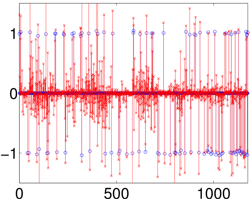
(a)

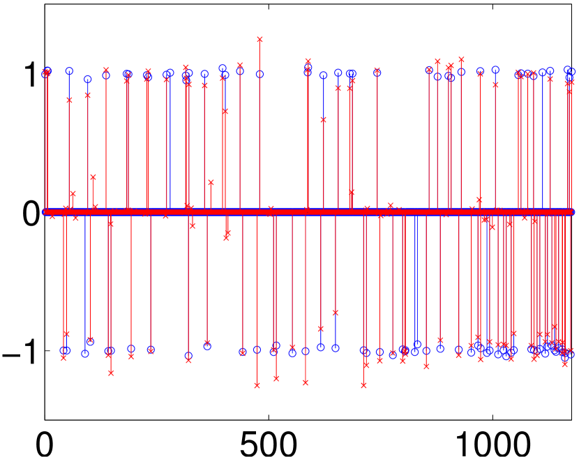
(b)

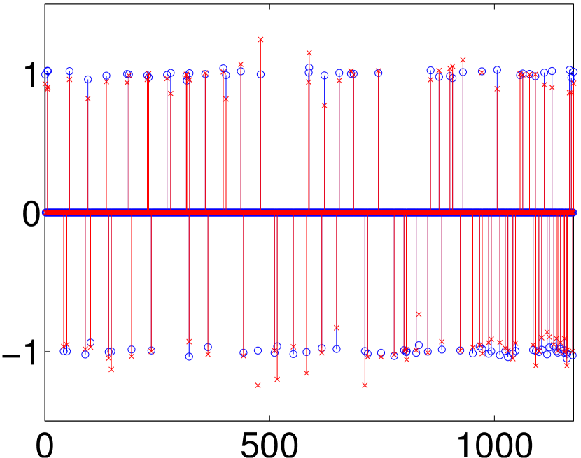
(c)

Figure 1: (Color online) True couplings (blue circles) compared with couplings inferred (red crosses) by maximizing likelihood method (a), $\ell_{1}$ minimization + refinement (b) and Decimation (c). The relative error (Eq. (11)) is $0.209$, $0.079$ and $0.026$ from left to right respectively. The network is a $2$D lattice with size $N=49$, $\beta=2.0$, $R=10$ and $T=500$.

Various approaches wainwright2010AnnalHigh ; cocco2011adaptive ; aurell2012inverse ; CoccoPNAS ; decelle13 have been proposed for the sparse inverse Ising problem, with different ways to overcome the over-fitting problem. Among various approaches, the probably most famous and effective one is based on the $\ell_{1}$-regularization wainwright2010AnnalHigh which consists in adding a prior on the couplings. This prior takes the form of a Laplace distribution on the parameters and usually leads to a sparse solution. As an example, in the middle panel of Fig.1 we compared the true couplings with the couplings inferred by the $\ell_{1}$ minimization approach on a sparse system. From the figure, we can see that the $\ell_{1}$ approach indeed recover much better the null couplings and give a smaller error than maximizing the likelihood alone. However, in our experiments, the $\ell_{1}$ approach still does not work perfectly, and fails to recover correctly the topology in many cases (even some easy ones). Moreover, its performance depends on an external parameter $\lambda$ that has to be chosen heuristically.

Recently, a decimation process was proposed in decelle13 for inferring the topology in the static inverse Ising problem. It was shown to give a large improvement over the reconstructed topology of the inference process over $\ell_{1}$-based methods. In the static problem, empirical data are equilibrium configurations that are sampled from the Boltzmann distribution $\mathcal{P}(\underline{\sigma})=\frac{1}{Z}e^{-\beta E(\underline{\sigma})}$, where $Z$ is the partition function and $E(\underline{\sigma})=-\sum_{\left\langle i,j\right\rangle}J_{ij}\sigma_{i}\sigma_{j}$ denotes the energy of a configuration $\underline{\sigma}$. When the number of samples is large, the couplings can be determined by maximizing the likelihood $\mathcal{L}(\underline{J})=-\left\langle E(\underline{J})\right\rangle_{D}-\log Z(\underline{J})$, where $\left\langle E\right\rangle_{D}$ denotes the averaged value of the energy over the data. In this setting however, the partition function $Z$ is hard to compute exactly to compute exactly and therefore the likelihood function is hard to compute as well (or to maximize). In decelle13 ; yamanaka2015detection , in order to use the decimation method, the authors needed to adopt the “pseudo-likelihood” which is essentially an approximation of the true likelihood function besag1975statistical ; ravikumar2010high .

In this work, we deal with the dynamical inverse Ising problem. This type of inference problem introduces a new sets of behavior that are absent of the static counter-part. Indeed, the configurations are now drawn from a stochastic process and are therefore correlated in time. From this stochastic process we expect the presence of relaxation toward an equilibrium distribution (somehow similar to the static inverse Ising case) but such systems also exhibit ergodicity breaking or limited cycles. In addition, it is more natural to describe many real systems by a dynamical process rather than by using an equilibrium distribution. For instance some biological systems depends on a time-dependent external stimuli. Moreover and as opposed to the static case, the couplings between the variables need not to be symmetric. Again, we show on the Fig. 1 right panel an illustration of this algorithm on the same system as before (see the caption) and we can see it manages to better recover the topology of the network than maximizing the likelihood alone.

The rest of the paper is organized as follows. Section II includes definitions and the description of the dynamical inverse Ising problem. In Sec. III we consider the dynamical inverse Ising problem on sparse graphs and review the popular $\ell_{1}$ based approach. In Sec. IV we study the inference of the couplings using the decimation process. In Sec. V we compare our method with the $\ell_{1}$ approach on a larger set of examples. We conclude this work in Sec. VI.

II The dynamical inverse Ising problem

The dynamical inverse Ising problem, first studied in Roudi_Hertz_PRL_106_048702 , asks to reconstruct the couplings and the time dependent external fields from output data of the real system. These data are sets of configurations which can be considered as a snapshot of the real system at different time steps. In our settings they are generated according to the dynamics of the Ising model with real couplings.

Let’s consider a system of $N$ nodes connected by the couplings $J_{ij}$. The state of each node is represented by a spin $\sigma$ that takes a discrete value in $\{-1,+1\}$. In eq. (1), we define a stochastic dynamics describing the evolution of a configuration of spins at time $t$ to one at time $t+1$. Here we consider the parallel update dynamics for which, the state of all spins at time $t+1$ depends only on the configuration at time $t$, and all spins evolve in parallel at the same time.

$$P(\sigma_{i}(t+1)|\underline{\sigma}(t))=\frac{\exp[\beta\sigma_{i}(t+1)\sum_{j\neq i}J_{ji}\sigma_{j}(t)]}{2\cosh(\beta\sum_{j\neq i}J_{ji}\sigma_{j}(t))}$$ (1)

Therefore, the probability of finding a particular path (a trajectory $\underline{\sigma}(0),...,\underline{\sigma}(T)$) with $T$ time-steps can be written as

$$W[\underline{\sigma}(T)|\underline{\sigma}(0)] = \prod_{t=0}^{T-1}\prod_{i=0}^{N-1}\frac{\exp[\beta\sigma_{i}(t+1)\sum_{j\neq i}J_{ji}\sigma_{j}(t)]}{2\cosh(\beta\sum_{j\neq i}J_{ji}\sigma_{j}(t))}$$ (2)

$$= \exp[\beta T\sum_{i}\sum_{j\neq i}J_{ji}\langle\sigma_{i}(t+1)\sigma_{j}(t)\rangle_{T}-\sum_{t,i}\log(2\cosh(\beta\sum_{j\neq i}J_{ji}\sigma_{j}(t)))]$$ (3)

where $\langle.\rangle_{T}$ means taking the average of the data over the different times: $\langle\sigma_{i}(t)\rangle_{T}=T^{-1}\sum_{t}\sigma_{i}(t)$. In general we consider not only the case with symmetric couplings where the detailed balance holds and the system has an equilibrium distribution, but also the case with non-symmetric couplings where no equilibrium distribution exists.

Note that, compared to the static inverse Ising problem where the couplings are symmetric and the data are sampled from the Boltzmann distribution, dynamical systems display a broader picture of phase diagram such as limited cycles or non-equilibrium steady states and thus obviously meet wider needs in real-world systems.

The log-likelihood function of this process is obtained by taking the logarithm of the expression (2). This function can be maximized simply by a gradient descent method, using the derivative of the log-likelihood with respect to the couplings. In the symmetric case we obtain:

$$\frac{1}{\beta T}\frac{\partial\log W}{\partial J_{ji}} = \left\langle\sigma_{i}(t+1)\sigma_{j}(t)\right\rangle_{T}+\left\langle\sigma_{j}(t+1)\sigma_{i}(t)\right\rangle_{T}-\left\langle\sigma_{j}(t)\tanh\left[\beta\sum_{k\neq j}J_{kj}\sigma_{k}(t)\right]\right\rangle_{T}-\left\langle\sigma_{i}(t)\tanh\left[\beta\sum_{k\neq i}J_{ki}\sigma_{k}(t)\right]\right\rangle_{T}$$ (4)

$$= c_{ij}^{\rm data}(t+1,t)+c_{ij}^{\rm data}(t,t+1)-c_{ij}^{J}(t+1,t)-c_{ij}^{J}(t,t+1),$$

which implies a moment-matching condition for the local maximum of the likelihood function:

$$c^{\rm data}_{ij}(t+1,t) = \left\langle\sigma_{i}(t+1)\sigma_{j}(t)\right\rangle_{T}$$ (5)

$$c_{ij}^{J}(t+1,t) = \left\langle s_{j}(t)\tanh\left[\beta\sum_{k\neq j}J_{kj}s_{k}(t)\right]\right\rangle_{T}.$$ (6)

In the non symmetric-coupling case, the equations take a simpler form:

$$\frac{1}{\beta T}\frac{\partial W}{\partial J_{ji}}=c_{ij}^{\rm data}(t+1,t)-c_{ij}^{J}(t+1,t).$$ (7)

So, starting from an initial condition, the couplings can be updated using the very general update rule: $J_{ij}^{\rm new}=J_{ij}^{\rm old}+\eta(c_{ij}^{\rm data}(t+1,t)-c_{ij}^{J}(t+1,t))$, where $\eta$ is the learning rate. In the following we will mainly concentrate on symmetric couplings but the generalization to non symmetric couplings is straightforward.

Note that, in the static case, the likelihood is a function of the correlations and therefore is difficult to maximize. It is even difficult to compute the likelihood exactly since the computational complexity is exponential in the system size. Here, as opposed to the static case, the likelihood of the dynamical model can be easily computed exactly with linear complexity in the number of samples and quadratic in the system size. Although several approximate methods have been studied in the literature Roudi_Hertz_PRL_106_048702 ; Mezard_Sakellariou_jstat_2011 ; zhang12 ; Sakellariou_etal_arxiv_2011 , using mean-field approximations to accelerate the inference process, in this paper we consider only exact likelihood-maximizing methods which compute the correlations exactly given a set of parameters.

Another difference between the dynamical and the static case comes from how the data are taken (or produced). In the static problem, the data are made of spin configurations sampled independently from the Boltzmann distribution. Thus the result does not depend on how the data are acquired, only the number of configurations matters. At the opposite, in the dynamical case, the configurations are generated through a stochastic markovian process. Therefore it is possible to control the way the data are produced by, for instance, making many sets of data starting from different initial conditions. This liberty is impossible in the static case and should in principle improve here the inference process for systems where the dynamics gets trapped into some region of the phase space.

Here we consider a collection of data parametrized by two variables: the number of different trajectories $R$ and the number of time steps $T$ of each trajectory. The total number of configurations is then equal to $R\times T$. In this way, we collect the data under the form of $R$ trajectories with length $T+1$ zhang12 , each of which starts from $R$ different randomly chosen configurations. For each trajectory we update $T$ times the system according to eq. (1). The $R$ parameter let us tune the position from which the dynamics began. It therefore allows to cover a larger part of the configuration space. For example, when $R=1$, all configurations are sampled starting from one initial configuration. In the generated data, it will be useful to use $R>1$ in order to explore better the phase space.

The $T$ parameter controls the number of time-steps of each trajectory. Again, in many cases, we gain more information on the system by considering many short trajectories instead of a long one. Now, when the system is ergodic, tuning the dynamics should not have any influence on the results since the configuration can go from any point of the configuration space to any other ones, which includes somehow already the new random initial conditions. But if the ergodicity does not hold, for example when the system is in a spin glass phase, a dynamics starting from a particular configuration could be trapped into a certain regime of the configuration space. Thus, starting from different configurations helps exploring wider area of the phase space and improves the data quality.

Let’s now rewrite the likelihood function in terms of the parameters $R$ and $T$. If we denote the sampled configurations by $\{\sigma^{a}(t)\}$, with $a\in[1,R]$ and $t\in[1,T+1]$, the likelihood function of generating those configurations can be written as

$$\mathcal{L} = \prod_{a=1}^{R}\prod_{t=1}^{T}W[\underline{\sigma}^{a}(t+1)|\underline{\sigma}^{a}(t)]$$ (8)

$$= \exp\left[\beta\sum_{i\neq j}J_{ji}\left\langle\langle\sigma_{i}(t+1)\sigma_{j}(t)\rangle_{T}\right\rangle_{R}-\sum_{a,t,i}\log(2\cosh(\beta\sum_{j\neq i}J_{ji}\sigma_{j}^{a}(t)))\right]$$

where the notation $\langle.\rangle_{R}$ is used to represent the average over the different realizations. Then, using a gradient descent, a set of couplings can be inferred by maximizing the above likelihood. As discussed previously, by maximizing this likelihood, we will not only fit the data but also the noise in the data. It will be particularly true in the cases where the dynamics gets trapped in some small region of the phase space, or when the number of samples $R\times T$ is small. Then, we will have difficulties in inferring the couplings as well as recovering the topology of the graph. In this work, in order to span a large region of the temperature $\beta$, we choose $R=10$ and $T=500$. This is equivalent of taking $R=1$ and $T=5000$ in term of the number of configurations that are visited. By doing this, however, we are exploring different regions of the phase space and therefore we are able to perform a better reconstruction.

III Dynamic Inverse Ising problem on sparse graphs

Most of the biological and social networks are sparse, meaning that the average degree of those networks is finite ($c<<N$ ). To do inference on sparse systems, it is very important to first determine which edges are present, or equivalently which couplings are non-zero. Therefore, when it is known as a prior that the underlying graph of a system is sparse, the correct Bayesian inference process should take into account this information under the form of a prior distribution. Ignoring this prior information when maximizing the likelihood will lead to over-fitting, as we discussed in Sec. I and shown in Fig. 1 left.

The $\ell_{1}$-regularization is a well-known method to obtain sparse solutions in inference problems. It has been widely used in compressed sensing donoho2006compressed and for the inverse Ising problems wainwright2010AnnalHigh ; tkavcik2014searching . The $\ell_{1}$-based methods consist in adding a Laplace prior: $e^{-\lambda\sum_{ij}|J_{ij}|}$ to the system, in order to obtain a sparse solution. The major advantage of the $\ell_{1}$ regularization is that, adding the Laplace prior does not break the convexity of the likelihood function. this method is fully tractable, there are several drawbacks. First, it is hard to fix the parameter $\lambda$ of the Laplace distribution consistently. When using a given value of $\lambda$, many couplings will be put to zero in the maximization process. It is possible to determine the maximum value of $\lambda$ analytically such that, for $\lambda>\lambda_{\rm max}$, all the inferred couplings will be zero. But then, the best value of $\lambda$ inside $[0,\lambda_{\rm max}]$ is not given by the $\ell_{1}$ method. Indeed, by changing the value of $\lambda$, the set of inferred zero-couplings will change accordingly and it is therefore not possible to know what would be the best value of $\lambda$. As an example, in Fig. 2, we plot the histogram of couplings inferred by maximizing the likelihood using a $\ell_{1}$ prior and using two different values of $\lambda$. We can see that, although it seems quite easy to choose the cut-off value on whether couplings are zero or not, different values of $\lambda$ give a different number of zero couplings and thus end with two different topologies for the network.

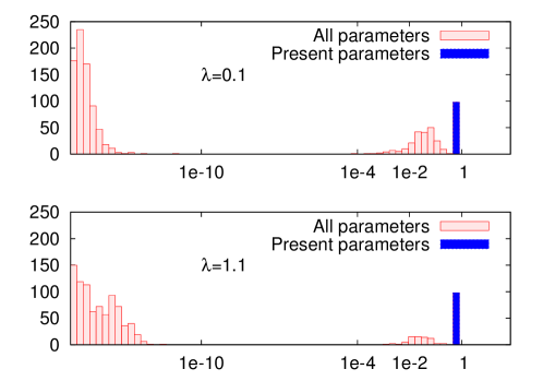
Figure 2: (Color online) Illustration of the results obtain by maximizing the likelihood together with the $\ell_{1}$ prior on a set of data generated by a parallel dynamics. The considered system is a 2D ferromagnet at low temperature, $\beta=0.61$ and we use $T=1000$ and $R=1$. The histograms show the parameters obtained for $\lambda=0.1$ (top) and $\lambda=1.1$ (bottom). Clearly the number of zero couplings change drastically when $\lambda$ changes.

Another drawback of the $\ell_{1}$ based-method is that the Laplace prior is sometimes far from the distribution of the true couplings. Thus the $\ell_{1}$ minimization will try to fit the couplings with a Laplace distribution and lead to additional errors. The Bayesian prescription advises us that using the correct prior is always the best choice to obtain the best performance, e.g. in compressed sensing problem PhysRevX.2.021005 , group testing problem pan_group_testing and error-correction problem error_correction_ITW2013 . However, in the inverse Ising problem, we usually cannot use the correct prior distribution because otherwise the problem would not be convex any more.

IV Decimation Process

Decimation methods have been widely use in statistical mechanics in various problems and it can be seen as a practical tool to reduce the seach space of our problem. This idea is actually quite old maslov , especially in the context of optimization problems. In the context of the inverse Ising problem and more generally in machine learning, this procedure can reduce greatly the overfitting over the inferred parameters. It was therefore used to reduce the number of parameters of the model to infer (see lecun1989optimal for method close to the one presented here). Another advantage of the decimation procedure is that, by reducing the search space, the system receives a feedback that it can exploit to solve the problem with more accuracy. This is typically used when solving constraint satisfaction problems using the marginals of the variables obtained by a message-passing algorithm ricci2009cavity ; mezard2002analytic .

For the inverse Ising problem, the decimation process was introduced to recover the topology of the Ising model and shown to provide a significant improvement on the quality of the reconstruction over the popular $\ell_{1}$-based methods decelle13 . In the static problem, since the real likelihood function is hard to estimate exactly, the decimation procedure is done by maximizing an approximation of the likelihood function (the pseudo-likelihood besag1975statistical ) and then by pruning a fraction of the smallest couplings (in magnitude) by setting their values to zero. This maximizing-pruning procedure is iterated until a given criterion is reached.

In the dynamical problem, as we discussed in the last section, the likelihood function can be easily estimated and thus the decimation can be applied directly by using the true likelihood function. The most intuitive way to fix the variables would be to set to zero one variable at a time after having maximized the likelihood function over the remaining parameters. However, in doing this way, the decimation would be very slow (it would multiply the complexity of the algorithm by a factor $\log(N)$). In order to make it fast without loosing accuracy, we can fix a finite fraction of variables at each time step. Doing so, the only parameter in our decimation procedure is the fraction of couplings that are pruned at each time-step. A refined way to choose this fraction is, at the first steps of the decimation, to prune a large amount of the remaining parameters. Then, the fraction of couplings to decimate is decreased gradually during the process.

We note that in the literature, another decimation approach has been proposed lecun1989optimal ; hassibi1993second in a different context. In their approach, instead of pruning the parameters by order of magnitude, the algorithm will in priority put to zero the parameters that decrease the least the likelihood function. Let’s assume for instance that the maximum of the likelihood function has been found. We can then make an expansion around this maximum ${J}^{*}$:

$$\mathcal{L}({J}^{*}+{\delta J})\sim\mathcal{L}({J}^{*})+\frac{1}{2}\delta{J}H\delta{J},$$ (9)

where $H$ is the Hessian of the likelihood function evaluated at ${J}^{*}$. The goal is then to find a set of couplings in such a way that putting them to zero will affect the least the likelihood function. Therefore it asks to minimize $L=\frac{1}{2}\delta{J}H\delta{J}$ such that $J_{i}+\delta J_{i}=0$ for the couplings that will be pruned. This second-order decimation process will be denoted as “Deci-O2” in the following and will be compared with our approach.

The most important step of the algorithm is to decide when to stop the decimation. We use here the same criterion as in decelle13 which is defined by investigating the behaviour of the likelihood function when we decimate the parameters.

To describe its principle, let us note the set of non-zero/zero couplings of the true system by $\bm{J_{1}}$/$\bm{J_{0}}$ respectively. One would expect the following. When a coupling $J_{ij}\in\bm{J_{0}}$ is pruned during the decimation process, the likelihood should remain constant as this parameter is not useful to describe the data. In practice, and due to the over-fitting phenomena, the likelihood will slightly decrease since the model is less accurate to fit the noise of the data. Now, if a coupling $J_{ij}\in\bm{J_{1}}$ is pruned, this parameter was necessary to describe correctly the data. Therefore its absence should impact the likelihood and we expect to observe its value to decrease significantly. Hence, by looking at the likelihood as a function of the number of the remaining parameters, we can find the stopping point where the behaviour of the likelihood changes significantly. That is, a discontinuity in the first derivative of the likelihood function should be observed.

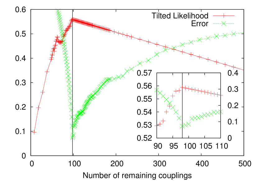
(a)

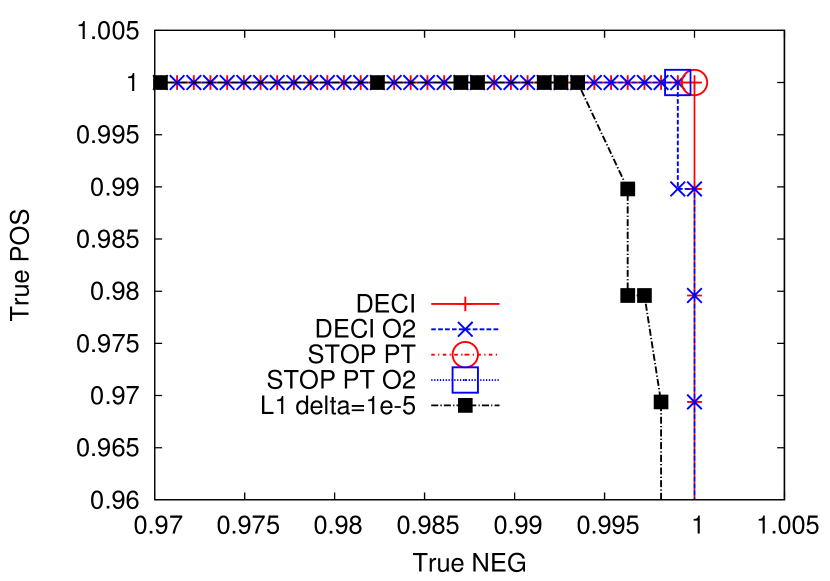
(b)

Figure 3: (Color online) (a): Illustration of a typical Tilted Likelihood (TL) function. In this case we are in a hard region, $N=49$, $\beta=1.5$ with $R=10$ and $T=500$ of a 2D symmetric model with $J=\pm 1$. We observe a well-defined peak which indicates where to stop the decimation process. In the inset we show that the relative error is minimized at the peak. In this case, the decimation process reconstructs perfectly the network as indicated in the right panel. (b): the ROC curve for the same system in the left panel. The ROC curves show the number of true positives on the y-axis and true negatives on the x-axis. The goal is therefore to reach the right-top angle for a perfect reconstruction. Here, the decimation process and the Deci-O2 method are shown at different stages of the decimation (at $T=0$ the curve start at (0,1)). For the $\ell_{1}$ method, different points correspond to different values of $\lambda$. We can see that, our method works better than the two other ones. The $\ell_{1}$ method is clearly less good even when considering the best possible $\lambda$ ($\delta$ indicates the value of the cut-off but is chosen such that it goes into the gap separating zero couplings from the non zero ones (see Fig. 2).

We will follow here the prescription of decelle13 in order to characterized the stopping point for the decimation. In order to exhibit a peak at the point where to stop the decimation, the following “tilted-Likelihood” (TL) function has been considered

$$\mathcal{L}^{\rm tilted}(x)=\mathcal{L}(x)-x\mathcal{L}_{\rm max}+(1-x)N\log(2),$$ (10)

where $\mathcal{L}_{\rm max}$ is the maximum likelihood when all the parameters are present (before decimating), and $x$ denotes the fraction of couplings that remain unfixed. We also note $\mathcal{L}(x)$ the maximum of the likelihood over the remaining parameters (note that $\mathcal{L}(0)$ is the usual maximum likelihood when all parameters are present). The TL is constructed as follows. We consider a new likelihood for a system of independent variables but where its maximum value when all the couplings are present ($x=0$) matches the likelihood of the system $\mathcal{L}(0)=\mathcal{L}_{\rm indep}(0)$. The likelihood of our system of independent variables should decrease linearly (with $x$) when decimating the parameters since they are here not useful to describe the system. When $x=1$, both likelihoods will reach the value $\mathcal{L}(1)=\mathcal{L}_{\rm indep}(1)=-\log(2)$ by definition. The TL is constructed by looking at the difference between the two likelihoods $\mathcal{L}_{\rm tilted}(x)=\mathcal{L}(x)-\mathcal{L}_{\rm indep}(x)$. It can be seen by this construction that the TL goes to zero when $x=1$ and $x=0$. Therefore it should exhibit a maximum value between these two limits. When we start decimation, since we expect to decimate couplings from $\bm{J_{0}}$ at the beginning, the likelihood of our system will remain almost constant while the likelihood of the system with independent variables will decrease more rapidly and make the TL increases. At a certain point, where we start to decimate parameters that are present in the true system, the likelihood of our system will decrease dramatically while the likelihood for the system of independent variables will keep decreasing at a constant rate. Therefore, a peak should appear at the point where the process starts to decimate the wrong parameters.

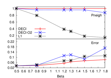
Figure 4: (Color online) Results obtained on a 2D symmetric model $J=\pm 1$ with $N=49$, $R=10$ and $T=500$ for various values of $\beta$. On the top panel, we can see the topology reconstruction (eq. 12) of the three methods : Decimation, Deci-O2 and $\ell_{1}$. We can see clearly that the decimation always recovers perfectly the topology of the graph whereas $\ell_{1}$ performs poorly. The Deci-O2 method works quite close to the decimation. On the bottom panel, we show the error on the reconstruction (eq. 11). All methods perform similarly with a slight advantage towards the decimation. This behaviour can be explain by the fact that, often, the error in the topology reconstruction is dominated by the false negative couplings. The $\ell_{1}$ finds a lot of false positives but they are inferred quite close to zero (i.e. their true value) and therefore they do not contribute much to the reconstruction error.

In order to illustrate the behavior of the TL in the whole decimation process we take a symmetric 2D Ising model with $N=49$ spins and $J=\pm 1$ at $\beta=1.5$. The decimation process is characterized by the function $K(T)$ which defines how many couplings we put to zero at each time-step. Here we define $K(T)$ in such a way that for small $T$ a large amount of couplings are decimated. Then, we progressively diminish the number of decimated couplings at each $T$ until the we end up decimating one coupling at each time-step, $K(T)=1$. This parametrization is quite flexible and we did not observe significant changes as soon as $K(T)$ was small enough after having decimated half of the system. We illustrate on Fig. 3 the behavior of the TL as a function of the remaining parameters. We can see that the TL exhibits a maximum at the point where the relative error, eq. (11), is minimized. On the right part of Fig. 3 we plot the ROC curve which puts the number of true positives on the y-axis versus and number of true negatives on the x-axis. In Fig. 4 we compare the performance of our method with Deci-O2 and the $\ell_{1}$ method in recovering the topology. The figure shows that our decimation method stopped at a point where the topology is perfectly reconstructed - making no false negative or false positive. The Deci-O2 works a bit worse than our method, making one false negative at its stopping point. The $\ell_{1}$ method works the worst, making lots of false negatives and false positives.

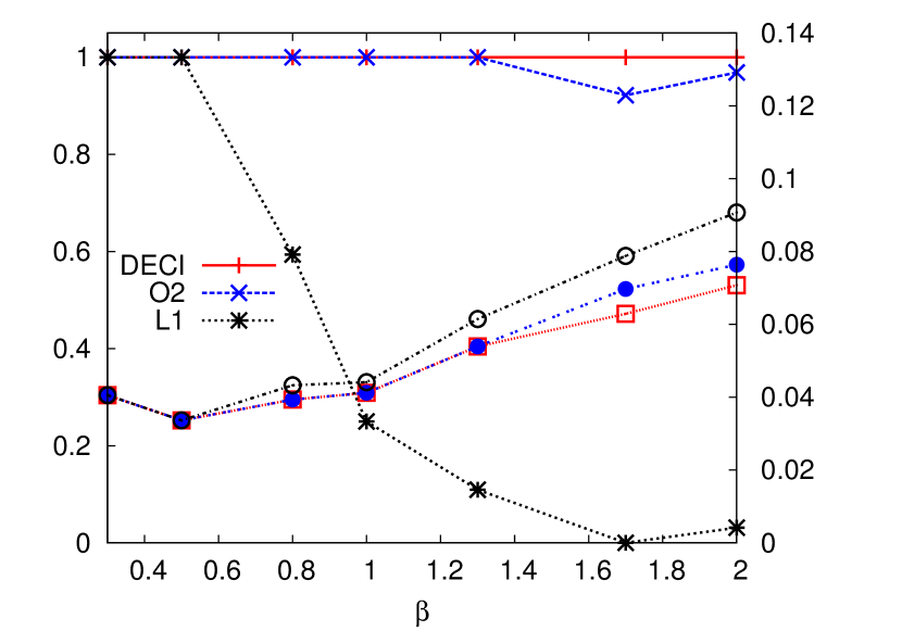
(a)

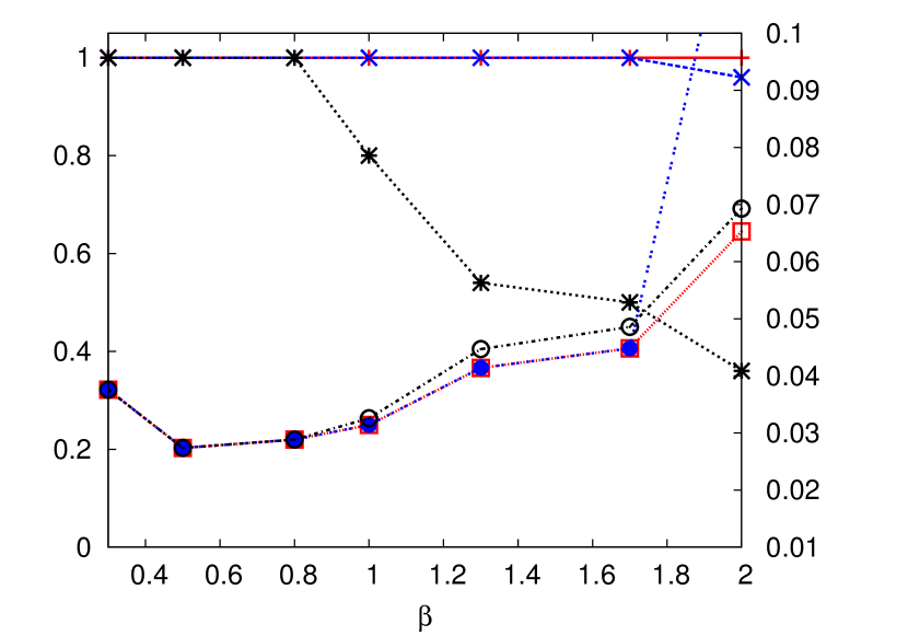
(b)

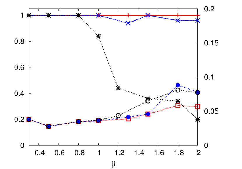
(c)

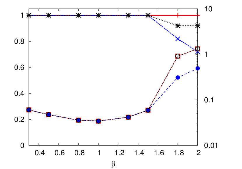
(d)

Figure 5: (Color online) Comparison of the performance of the three methods on different topologies: (a) 3D lattice with $N=64$, $J=\pm 1$, $R=10$ and $T=500$; (b) ER random graph with $N=50$, $J=\pm 1$, $R=10$ and $T=500$; (c) Gaussian couplings on a random graph with $N=50$, $\sigma_{\rm Gauss}=0.1$, $R=10$ and $T=500$; (d) Asymmetric couplings with $J_{ij}=\pm 1$ on a random graph with $N=50$, $R=1$ and $T=5000$. In each figure the crosses correspond to the value of $P_{\rm neigh}$ (Eq. (11)), the circles and the squares correspond to the relative error $\epsilon$ (Eq. (11)). From those figures we can conclude that the decimation works always much better than the $\ell_{1}$ method. The Deci-O2 method is comparable but always slightly worse than the decimation. The details concerning the comparison are described in the text.

V Numerical results and performance comparison

In this section we systematically study the performance of the proposed method and we compared it with the $\ell_{1}$ method and the Deci-O2 method on various topologies and with various parameters of the kinetic Ising model. These systems include $\pm J$ and Gaussian-distributed couplings, on 2D lattices and on ER random graphs. Concerning the decimation-based methods (decimation and Deci-O2) at each time-step the likelihood is maximized over the remaining couplings and a fraction of couplings is put to zero. Our only free parameter was the fraction of decimated couplings at each time-step. Concerning the $\ell_{1}$ method, the likelihood together with the Laplace prior was maximized for a set of $\lambda$ chosen inside $[0,\lambda_{\rm max}]$. Then, the value of $\lambda$ where the ROC curve was the closest to the perfect reconstruction was chosen. We should emphasize that this choice is highly non trivial and it would not be possible to do the same in many real inference problems. Finally, the topology is reconstructed by taking a cutoff inside the gap separating the zero couplings from the others (see Fig. 2 for the gap). The error on the reconstruction is computed over a new maximization of the likelihood, this time without the Laplace prior but with the previously inferred topology. This last step is done in order to not bias the value of the inferred couplings because of the $\ell_{1}$ penalty term.

To evaluate the performance we consider two measures. The first measure is the relative error of the reconstruction which is defined as

$$\epsilon=\sqrt{\frac{\sum_{i<j}\left(J_{ij}-J_{ij}^{*}\right)^{2}}{\sum_{i<j}J_{ij}^{2}}}.$$ (11)

The second measure takes into account the reconstruction of the topology by counting the number of well-reconstructed neighborhoods. For each site $i$, the neighborhood of $i$ is said to be reconstructed if, for all the couplings $J_{ij}$, $\forall j\neq i$, the inference process has separated correctly the zero couplings from the present ones. We then sum over all the sites to obtain the measure

$$P_{\rm neigh}(\{J^{*}\})=\frac{1}{N}\sum_{i=1}^{N}\delta\left(\sum_{\underset{J_{ij}\in\bm{J}_{1}}{j\neq i}}\delta_{J^{*}_{ij},0}+\sum_{\underset{J_{ij}\in\bm{J}_{0}}{j\neq i}}(1-\delta_{J^{*}_{ij},0})\right)..$$ (12)

This observable is zero if at least one error is made for all the neighborhoods, and is one if all the neighborhoods are reconstructed perfectly. The results are illustrated on Fig. 5. We can see from the figures that on various topologies and parameters, the decimation algorithm clearly recovers the topology in all cases. In comparison, the $\ell_{1}$ method does not work well to recover the topology and usually finds slightly larger errors. However, it is interesting to understand why the error in the $\ell_{1}$ method performs as well as in the decimation and Deci-O2 cases while the reconstructed topology is completely wrong. First of all, the reconstructed topology is mainly affected by the fact that the $\ell_{1}$ method is unable to find correctly who are the zero couplings of the system. It means that, this method, even by tuning the value of $\lambda$ (as we did here) is not close to the correct solution in many cases. But, as the topology is wrong mainly because of the false positives, the inferred value of these couplings will remain close to zero and therefore they do not contribute significantly to the relative error. Finally it is also interesting to see that the Deci-O2 method has a behaviour very similar to the one of the decimation while always slightly worse than our method, especially in the topology reconstruction.

VI Conclusion and discussion

In this paper we proposed a simple method based on a decimation process to the inference of the dynamical inverse Ising problem on sparse graphs. We claim that our method is a much more robust approach than the maximum-likelihood method, which is prone to overfitting. In addition, unlike the $\ell_{1}$ approach, we do not assume an artificial prior on the couplings, and we do not have any parameter to tune. Experimental results show that our method outperforms $\ell_{1}$-based method on various topologies and with different coupling distributions. It also shows improvement over a decimation based method using the second derivative of the likelihood function.

Including our method, many existing approaches to the inverse Ising problems are based on a “maximum à posterior” method. However, in cases where the amount of data is small or when the data quality is low, it would be very helpful to develop a real Bayesian inference method considering the average over all possible couplings and not focusing on the value of the couplings that maximize the posterior distribution. We leave this for future work.

Though all the study in this paper is theoretical, we note that it would be very interesting to test our method on real-world problems, probably with missing or noisy data. We leave this for future work.

- [1] David H Ackley, Geoffrey E Hinton, and Terrence J Sejnowski. A learning algorithm for boltzmann machines. Cognitive science, 9(1):147–169, 1985.
- [2] Elad Schneidman, Michael J. Berry, Ronen Segev, and William Bialek. Weak pairwise correlations imply strongly correlated network states in a neural population. Nature, 440:1007–1012, 2006.
- [3] Erik Aurell and Magnus Ekeberg. Inverse ising inference using all the data. Phys. Rev. Lett., 108:090201, Mar 2012.
- [4] H. Chau Nguyen and J. Berg. Bethe-peierls approximation and the inverse ising model. arXiv, 1112.3501, 2011.
- [5] H. Chau Nguyen and J. Berg. Mean-field theory for the inverse ising problem at low temperatures. arXiv, 1204.5375, 2012.
- [6] Federico Ricci-Tersenghi. On mean-field approximations for estimating correlations and solving the inverse ising problem. arXiv preprint arXiv:1112.4814, 2011.
- [7] Aurélien Decelle and Federico Ricci-Tersenghi. Pseudolikelihood decimation algorithm improving the inference of the interaction network in a general class of ising models. Phys. Rev. Lett., 112:070603, Feb 2014.
- [8] B. Ravikumar, M.J. Wainwright, and J.D. Lafferty. High-dimensional ising model selection using l1-regularized logistic regression. The Annals of Statistics, 38, 2010.
- [9] Gonzalo A Ruz and Eric Goles. Learning gene regulatory networks with predefined attractors for sequential updating schemes using simulated annealing. In Machine Learning and Applications (ICMLA), 2010 Ninth International Conference on, pages 889–894. IEEE, 2010.
- [10] Martin Weigt, Robert A White, Hendrik Szurmant, James A Hoch, and Terence Hwa. Identification of direct residue contacts in protein–protein interaction by message passing. Proceedings of the National Academy of Sciences, 106(1):67–72, 2009.
- [11] Magnus Ekeberg, Cecilia Lövkvist, Yueheng Lan, Martin Weigt, and Erik Aurell. Improved contact prediction in proteins: Using pseudolikelihoods to infer potts models. Physical Review E, 87(1):012707, 2013.
- [12] Gašper Tkačik, Elad Schneidman, II Berry, J Michael, and William Bialek. Ising models for networks of real neurons. arXiv preprint q-bio/0611072, 2006.
- [13] Santo Fortunato. Community detection in graphs. Physics Reports, 486(3):75–174, 2010.
- [14] William Bialek, Andrea Cavagna, Irene Giardina, Thierry Mora, Edmondo Silvestri, Massimiliano Viale, and Aleksandra M Walczak. Statistical mechanics for natural flocks of birds. Proceedings of the National Academy of Sciences, 109(13):4786–4791, 2012.
- [15] S. Cocco and R. Monasson. Adaptive cluster expansion for inferring boltzmann machines with noisy data. Phys. Rev. Lett., 106:090601, Mar 2011.
- [16] Simona Cocco, Stanislas Leibler, and Rémi Monasson. Neuronal couplings between retinal ganglion cells inferred by efficient inverse statistical physics methods. Proceedings of the National Academy of Sciences, 106(33):14058–14062, 2009.
- [17] Shogo Yamanaka, Masayuki Ohzeki, and Aurélien Decelle. Detection of cheating by decimation algorithm. Journal of the Physical Society of Japan, 84(2), 2015.
- [18] Julian Besag. Statistical analysis of non-lattice data. The statistician, pages 179–195, 1975.
- [19] Pradeep Ravikumar, Martin J Wainwright, John D Lafferty, et al. High-dimensional ising model selection using ℓ1-regularized logistic regression. The Annals of Statistics, 38(3):1287–1319, 2010.
- [20] Yasser Roudi and John Hertz. Mean field theory for nonequilibrium network reconstruction. Phys. Rev. Lett., 106(4):048702, Jan 2011.
- [21] M. Mezard and J. Sakellariou. Exact mean field inference in asymmetric kinetic ising systems. J. Stat. Mech., L07001, 2011.
- [22] Pan Zhang. Inference of kinetic ising model on sparse graphs. Journal of Statistical Physics, 148(3):502–512, 2012.
- [23] Jason Sakellariou, Yasser Roudi, Marc Mezard, and John Hertz. Effect of coupling asymmetry on mean-field solutions of direct and inverse sherrington-kirkpatrick model. arXiv, 1106.0452, 2011.
- [24] David L Donoho. Compressed sensing. Information Theory, IEEE Transactions on, 52(4):1289–1306, 2006.
- [25] Gašper Tkačik, Olivier Marre, Dario Amodei, Elad Schneidman, William Bialek, and Michael J Berry II. Searching for collective behavior in a large network of sensory neurons. PLoS computational biology, 10(1):e1003408, 2014.
- [26] F. Krzakala, M. Mézard, F. Sausset, Y. F. Sun, and L. Zdeborová. Statistical-physics-based reconstruction in compressed sensing. Phys. Rev. X, 2:021005, May 2012.
- [27] Pan Zhang, F. Krzakala, M. Mezard, and L. Zdeborova. Non-adaptive pooling strategies for detection of rare faulty items. In Communications Workshops (ICC), 2013 IEEE International Conference on Communications, pages 1409–1414, June 2013.
- [28] Jean Barbier, Florent Krzakala, Lenka Zdeborova, and Pan Zhang. Robust error correction for real-valued signals via message-passing decoding and spatial coupling. In Information Theory Workshop (ITW), 2013 IEEE, pages 1–5, Sept 2013.
- [29] Sergeǐ Yu Maslov, Vladimir Lifschitz, and Michael Gelfond. Theory of deductive systems and its applications. MIT Press, 1987.
- [30] Yann LeCun, John S Denker, Sara A Solla, Richard E Howard, and Lawrence D Jackel. Optimal brain damage. In NIPs, volume 2, pages 598–605, 1989.
- [31] Federico Ricci-Tersenghi and Guilhem Semerjian. On the cavity method for decimated random constraint satisfaction problems and the analysis of belief propagation guided decimation algorithms. Journal of Statistical Mechanics: Theory and Experiment, 2009(09):P09001, 2009.
- [32] Marc Mézard, Giorgio Parisi, and Riccardo Zecchina. Analytic and algorithmic solution of random satisfiability problems. Science, 297(5582):812–815, 2002.
- [33] Babak Hassibi, David G Stork, et al. Second order derivatives for network pruning: Optimal brain surgeon. Advances in neural information processing systems, pages 164–164, 1993.