Problems of interaction of a supersonic gas mixture with a wall solved by the projection method applied to the full Boltzmann equation

1 Introduction

Our approach to problems of rarefied gas dynamics is based on direct solution of the complete kinetic Boltzmann equation. The main difficulty of solving the Boltzmann equation is the calculation of the multi-dimensional collision integral. In this paper, we apply our generalization of the conservative discrete ordinate method of Tcheremissine [1] (which was originally developed for a single gas) for binary gas mixtures in the case of cylindrical symmetry (Raines A. A.) [2]. For the evaluation of collision integrals we use the projection method which ensures the strict conservation of mass, momentum and energy. The conservativeness of the method is achieved by a special projection of the integrand values, calculated at non-node points, to nodes of the momentum grid that are closest to them.

Using this method, we now solve the problem of interaction of a two-component supersonic jet with a normally posed wall. We discover the effects of the inflow of gas on a cool wall with the mirror and diffuse reflection laws and the appearance of the wall Knudsen layer. The results are compared with the gas-dynamical solution and with the papers dealing with a similar problem for a single gas [3, 4]. We obtain a good agreement with all those results.

2 Description of the method

The system of the Boltzmann equations in the momentum space for two gas components consisting of hard sphere molecules with the masses $m_{i}$ and diameters $d_{i}$ reads

$$\frac{\partial f_{i}}{\partial t}+\frac{\vec{p}}{m_{i}}\,\frac{\partial f_{i}}{\partial\vec{x}}=-L_{i}+G_{i},\qquad i=1,2,$$ (1)

where $f_{i}$ is the distribution function which depends on the vector of momentum $\vec{p}$, the vector of configuration space $\vec{x}$ and the time $t$.

Direct and reverse collision integrals have the form

$$L_{i}=\sum_{j=1}^{2}\int\limits_{-\infty}^{+\infty}\int\limits_{0}^{2\pi}\int\limits_{0}^{\pi}f_{i}f_{j^{\ast}}\frac{1}{2}\left(\frac{d_{i}+d_{j}}{2}\right)^{2}q_{ji}\sin{\theta}d\theta d\varphi d\vec{p}_{\ast}$$ (2)

$$G_{i}=\sum_{j=1}^{2}\int\limits_{-\infty}^{+\infty}\int\limits_{0}^{2\pi}\int\limits_{0}^{\pi}f^{\prime}_{i}f^{\prime}_{j^{\ast}}\frac{1}{2}\left(\frac{d_{i}+d_{j}}{2}\right)^{2}q_{ji}\sin{\theta}d\theta d\varphi d\vec{p}_{\ast}$$ (3)

$$q_{ij}=|(\vec{g}_{ji}\cdot\vec{n})|.$$

In the kinetic momentum space we have the following relations between the vectors of momentum before and after the collision

$$\vec{p}^{\prime}=\vec{p}+\frac{2m_{i}m_{j}}{(m_{i}+m_{j})}\,(\vec{g_{ji}}\cdot\vec{n})\vec{n}$$

$$\vec{p}^{\prime}_{\ast}=\vec{p}_{\ast}-\frac{2m_{i}m_{j}}{(m_{i}+m_{j})}\,(\vec{g_{ji}}\cdot\vec{n})\vec{n}$$ (4)

$$\vec{g_{ji}}=\frac{\vec{p}_{\ast}}{m_{j}}-\frac{\vec{p}}{m_{i}}$$

$$\vec{n}=\vec{n}(\cos\theta,\sin\theta\cos\varphi,\sin\theta\sin\varphi).$$

Here $\vec{n}$ is a unit vector directed along the interaction line of molecules, $\vec{g}_{ji}$ is their relative velocity, $\theta$ and $\varphi$ are collision angles.

We introduce in the limited domain of the configuration space a fixed grid. We impose limits on the momentum variables in (1) - (3) by introducing a domain $\Omega$ of volume $V$. In $\Omega$ we construct a discrete grid containing $N_{0}$ equidistant points $\vec{p}_{\beta}$ with the step $h$ which results in the discretization of the distribution functions and collision integrals as follows

$$f_{i}(\vec{p}^{\ast})=\frac{V}{N_{0}}\sum\limits_{\beta=1}^{N_{0}}f_{i\beta}\delta(\vec{p}^{\ast}-\vec{p}_{\beta})$$ (5)

$$L_{i}(\vec{p}^{\ast})=\frac{V}{N_{0}}\sum\limits_{\beta=1}^{N_{0}}L_{i\beta}\delta(\vec{p}^{\ast}-\vec{p}_{\beta})$$ (6)

$$G_{i}(\vec{p}^{\ast})=\frac{V}{N_{0}}\sum\limits_{\beta=1}^{N_{0}}G_{i\beta}\delta(\vec{p}^{\ast}-\vec{p}_{\beta})$$ (7)

The Boltzmann equation in a discrete form becomes

$$\frac{\partial f_{i\beta}}{\partial t}+\frac{\vec{p}_{\beta}}{m_{i}}\frac{\partial f_{i\beta}}{\partial\vec{x}}=-L_{i\beta}+G_{i\beta}$$ (8)

Equation (8) is solved by the splitting procedure. On each interval $\Delta t$ we split the process into the two stages, free-molecular flow and collisional relaxation described by the following equations

$$\frac{\partial f_{i\beta}}{\partial t}+\frac{\vec{p}_{\beta}}{m_{i}}\frac{\partial f_{i\beta}}{\partial\vec{x}}=0$$

$$\frac{\partial f_{i\beta}}{\partial t}=-L_{i\beta}+G_{i\beta}$$

Let us consider the integral operator

$$\Omega_{i}(\Phi)=\sum\limits_{j=1}^{2}\int\limits_{-\infty}^{+\infty}\int\limits_{-\infty}^{+\infty}\int\limits_{0}^{2\pi}\int\limits_{0}^{\pi}\Phi f_{i}f_{j^{\ast}}\frac{1}{2}\left(\frac{d_{i}+d_{j}}{2}\right)^{2}q_{ji}\sin\theta d\theta d\varphi d\vec{p}_{\ast}d\vec{p}$$

Taking for $\Phi$ a three-dimensional $\delta$-function, we reduce the collison integrals to the form

$$L_{i}(\vec{p}^{\,\ast})=\frac{1}{2}\Omega_{i}\big{(}\delta(\vec{p}^{\,\ast}-\vec{p})+\delta(\vec{p}^{\,\ast}-\vec{p}_{\ast})\big{)}$$ (9)

$$G_{i}(\vec{p}^{\,\ast})=\frac{1}{2}\Omega_{i}\big{(}\delta(\vec{p}^{\,\ast}-\vec{p}^{\,\prime})+\delta(\vec{p}^{\,\ast}-\vec{p}^{\,\prime}_{\ast})\big{)}$$ (10)

Transforming the integral operator to cylindrical coordinates and taking into account the relations $\vec{p}=\vec{p}(p,\rho,\gamma)$, $d\vec{p}=\rho dpd\rho d\gamma$ we obtain

$$\Omega_{i}(\Phi)=\sum\limits_{j=1}^{2}\,\int\limits_{\Omega\times\Omega}\int\limits_{0}^{2\pi}\int\limits_{0}^{\pi}\Phi f_{i}f_{j^{\ast}}\frac{1}{2}\left(\frac{d_{i}+d_{j}}{2}\right)^{2}q_{ji}\chi\sin\theta d\theta d\varphi d\vec{p}_{\ast}d\vec{p}$$

Introduce the uniform integration grid: $p_{\alpha\nu}$, $\rho_{\alpha\nu}$, $p_{\beta\nu}$, $\rho_{\beta\nu}$, $\gamma_{\nu}$, $\gamma_{\ast\nu}$, $\theta_{\nu}$, $\varphi_{\nu}$ with $N_{\nu}$ nodes. The multiple integral is calculated as the $8$-fold sum over all the nodes while the distribution functions do not depend on $\gamma_{\nu}$, $\gamma_{\ast\nu}$:

$$\tilde{L}_{i}(\vec{p}^{\,\ast})=A\sum\limits_{\nu=1}^{N_{\nu}}\sum\limits_{j=1}^{2}J_{\nu}^{ij}\big{(}\delta(\vec{p}^{\,\ast}-\vec{p}_{\alpha_{\nu}})+\delta(\vec{p}^{\,\ast}-\vec{p}_{\beta_{\nu}})\big{)}$$ (11)

$$\tilde{G}_{i}(\vec{p}^{\,\ast})=A\sum\limits_{\nu=1}^{N_{\nu}}\sum\limits_{j=1}^{2}J_{\nu}^{ij}\big{(}\delta(\vec{p}^{\,\ast}-\vec{p}^{\,\prime}_{\alpha_{\nu}})+\delta(\vec{p}^{\,\ast}-\vec{p}^{\,\prime}_{\beta_{\nu}})\big{)}$$ (12)

where

$$J_{\nu}^{ij}=f_{i\alpha_{\nu}}f_{j\beta_{\nu}}\frac{1}{2}\left(\frac{d_{i\alpha_{\nu}}+d_{j\beta_{\nu}}}{2}^{2}\right)q_{j\beta_{\nu}i\alpha_{\nu}}sin{\theta_{\nu}}\rho_{\alpha_{\nu}}\rho_{\beta_{\nu}},\quad A=V^{2}\pi^{2}/N_{\nu}$$

Combining (6) and (11) we obtain

$$\tilde{L}_{i\beta}=B\sum\limits_{\nu=1}^{N_{\nu}}\sum\limits_{j=1}^{2}\left(J_{\nu}^{ij\prime}+J_{\nu}^{ij\prime\prime}\right),\quad B=V\pi^{2}/(N_{\nu}/N_{0})$$ (13)

We replace the expressions in parentheses in (12) by using the relations

$$\delta(\vec{p}^{\,\ast}-\vec{p}^{\,\prime}_{\alpha_{\nu}})+\delta(\vec{p}^{\,\ast}-\vec{p}^{\,\prime}_{\beta_{\nu}})=\sum\limits_{\vec{s}}r_{\vec{s}}\big{(}\delta(\vec{p}^{\,\ast}-\vec{p}_{\lambda_{\nu}+\vec{s}})+\delta(\vec{p}^{\,\ast}-\vec{p}_{\mu_{\nu}+\tilde{\vec{s}}})\big{)}$$ (14)

The coefficients $r_{\vec{s}}$ can be found from the conditions of conservation of the density, kinetic momentum and energy in the decomposition (14) for a pair of cells including their vertices. For economy of computations it would be preferable to have a decomposition with a minimum number of terms, so that expression (14) becomes

$$\delta(\vec{p}^{\,\ast}-\vec{p}^{\,\prime}_{\alpha_{\nu}})+\delta(\vec{p}^{\,\ast}-\vec{p}^{\,\prime}_{\beta_{\nu}})=(1-r_{\vec{s}^{\ast}})\big{(}\delta(\vec{p}^{\,\ast}-\vec{p}_{\lambda_{\nu}})+\delta(\vec{p}^{\,\ast}-\vec{p}_{\mu_{\nu}})\big{)}$$

$$+r_{\vec{s}^{\ast}}\big{(}\delta(\vec{p}^{\,\ast}-\vec{p}_{\lambda_{\nu}+\vec{s}^{\ast}})+\delta(\vec{p}^{\,\ast}-\vec{p}_{\mu_{\nu}+\tilde{{\vec{s}}^{\ast}}})\big{)}$$ (15)

If we use (15) in (12) and combine with (7), then we obtain

$$\tilde{G}_{i\beta}=B\sum\limits_{\nu=1}^{N_{\nu}}\sum\limits_{j=1}^{2}\left[\left(J_{\nu}^{ij\prime}+J_{\nu}^{ij\prime\prime}\right)(1-r_{\nu})+\left(J_{\nu}^{ij\ast}+J_{\nu}^{ij\ast\ast}\right)r_{\nu}\right]$$ (16)

The expressions (13) and (16) define the conservative discrete ordinate method if the coefficients have been already found.

3 Formulation of the problem

Consider the problem of the inflow of a binary gas mixture upon a wall with mirror and diffusive laws of reflection of the gas from the wall. The half-space $x>0$ is being filled with the gas moving with velocity $U$ (or momentum $P$) in the negative direction of the $x$-axis. The density and temperature of the gas are equal to $n_{0}$ and $T_{0}$, respectively. At the instant $t=0$ we set an immovable wall at the point $x=0$. At $t>0$ the interaction of the gas with the wall starts. The system of Boltzmann equations in momentum space for this problem for the two gas components consisting of hard sphere molecules with masses $m_{i}$ and diameters $d_{i}$ has the form (1).

A solution of the problem depends on four variables, so that the distribution functions have the form $f_{i}=f_{i}(t,x,p,\rho)$. As an initial condition for the distribution functions we take Maxwell functions with parameters of the unperturbed flow

$$f_{i}(t=0,x,p,\rho)=n_{i0}\left(\frac{1}{2\pi kT_{0}m_{i}}\right)^{3/2}\exp{\left(-\frac{(p-m_{i}P/m)^{2}+\rho^{2}}{2km_{i}T_{0}}\right)},$$ (17)

where $n_{i0}$ is the number density of $ith$ component of the mixture, $n_{0}=n_{10}+n_{20}$, $m$ is mass of the mixture. For the calculations, an infinite domain of the variation of $x$ is replaced by the segment $[0,L]$ and at $x=L$ we set up conditions (17) for molecules flying into the domain, which yields a boundary condition on the free boundary surface

$$f_{i}\!\left(t=0,x=L,p<0,\rho\right)=n_{i0}\left(\frac{1}{2\pi kT_{0}m_{i}}\right)^{3/2}\times$$

$$\qquad\qquad\qquad\exp{\left(-\frac{(p-m_{i}P/m)^{2}+\rho^{2}}{2km_{i}T_{0}}\right)}.$$ (18)

On the left boundary of domain $[0,L]$ we set up conditions for $p\geqslant 0$. In the case of mirror reflection from the wall, the boundary conditions have the form

$$f_{im}\!\left(t=0,x,p\geqslant 0,\rho\right)=f_{i}(t,x,-p,\rho).$$ (19)

For diffusive reflection with the full accommodation the distribution functions of reflected molecules are assumed to be maxwellian with the temperature equal to the wall temperature:

$$f_{iw}(t,x=0,p\geqslant 0,\rho)=n_{iw}\left(\frac{1}{2\pi kT_{w}m_{i}}\right)^{3/2}\exp{\left(-\frac{p^{2}+\rho^{2}}{2km_{i}T_{w}}\right)}.$$ (20)

Here $T_{w}$ is the wall temperature, $n_{iw}$ is the density of reflected molecules which is found from the condition of non-percolation:

$$n_{iw}=-\frac{2\sqrt{\pi}}{\sqrt{2km_{i}T_{w}}}\iiint\limits_{p<0}f_{i}p\,d\vec{p}.$$

Thus, the problem of the inflow of a rarefied gas on a wall is posed for system (1) with initial conditions (17), boundary conditions (18) on the free boundary surface and boundary conditions (19), (20) on a solid wall. Graphical representation of solution results can be seen in figures 1–6.

4 Dimensionless quantities

Here we introduce the dimensionless quantities corresponding to all physical variables which are involved in our solution method.

$$c_{0}=\sqrt{\frac{2kT_{0}}{m_{1}}},\qquad p_{0}=\sqrt{2kT_{0}m_{1}}$$

$$\lambda=1/(\sqrt{2}\pi d_{1}^{2}n_{0}),\qquad\tau=\lambda/c_{0}$$

$$\vec{p}^{\,\prime}=\vec{p}/p_{0},\quad\vec{u}^{\,\prime}/c_{0},\quad t^{\prime}=t/\tau,\quad X^{\prime}=x/\lambda,\quad f_{i}/(n_{0}p_{0}^{-3})=f_{i}^{\prime}$$

$$n^{\prime}=n/n_{0},\quad T^{\prime}=T/T_{0},\quad q^{\prime}=q/(n_{0}p_{0}^{3}m_{1}^{-2})$$

$$P^{\prime}=-\frac{3\sqrt{5}}{4\sqrt{6}}\frac{(M^{2}-1)}{M}\sqrt{M_{x}},\quad U^{\prime}=-\frac{3\sqrt{5}}{4\sqrt{6}}\frac{(M^{2}-1)}{M}\frac{1}{\sqrt{M_{x}}}.$$

$$M=Mach,\qquad M_{x}=m_{mix}/m_{1}.$$

5 Parameters of calculations

All calculations were performed at the laptop computer Sony VAIO, processor Intel(R) Core(TM) 2CPU, 1.66GHz + 1.66GHz, 1.00GB of RAM.

Time for an iteration step is 2.4 sec., time for the whole problem until $t=30\tau$ is 120min ($\tau$ is the mean free time).

Numerical parameters of calculations:

$$M=2.8773,\quad U=-2,\quad m_{2}/m_{1}=0.5,$$

$$n_{2_{0}}/n_{1_{0}}=0.5/0.5,\quad d_{2}/d_{1}=1,Kn=1.$$

The grids used for calculations:
$Np\rho=1250=(25+25)25$ - the number of nodes of the momentum grid with the step $h=0.2$
$NX=180$ - the number of nodes of the $x$-grid with the step $h_{x}=0.2$.
$NOD=66000$ integration nodes, $DT=0.01$ is the time step.

6 Comparison of numerical results with the gas-dynamical solution

According to gas dynamics equations, a domain is created with constant values of macroscopic parameters behind the reflected shock wave. For parameters specified in section 5 this gas-dynamical solution is the following

$$n_{gd}=2.936,\quad n_{1gd}=n_{2gd}=1.468,\quad T_{gd}=3.4396$$

Here $n_{gd},n_{1gd},n_{2gd}$ are numerical densities of the mixture, first component, and second component, respectively, while $T_{gd}$ is the temperature of the mixture.

Our results obtained by the direct numerical solution of the Boltzmann equation are described below.

1. Mirror reflection.
When $T_{wall}=T_{gas}=1$, there is the zone of constant values for density and temperature

$$n=2.93598,\quad n_{1}=1.48607,\quad n_{2}=1.451$$

$$T=3.44089,\quad T_{1}=3.44135,\quad T_{2}=3.4375.$$

2. Diffusive reflection.
a) When $T_{wall}=0.5$, $T_{gas}=1$ and $t>18\tau$, $x>12.5\lambda$, we have the region of constant values for density and temperature

$$n=2.9348,\qquad T=3.3435.$$

b) When $T_{wall}=T_{gas}=1$ and $t>18\tau$, $x>12.5\lambda$ we have the region of constant values for density and temperature

$$n=2.9313,\qquad T=3.3135.$$

We observe a good agreement of our results with the gas-dynamical solution.

7 Comparison of our results with the results obtained by other methods

Among other publications studying this problem, we should mention two earlier works that restrict themselves to a one-component gas [3, 4]. In [3], a conservative difference scheme is applied for solving the Boltzmann kinetic equation by the splitting method, with a good agreement of results shown in Figure 7. In [4] a scheme of the second order of accuracy with respect to $\Delta t$ is applied on the basis of the model Krook equation. For the sake of comparison with [4] we have solved the problem of reflection of a shock wave from a wall with a reasonable agreement of our result with [4] shown in Figure 8. Initial test of the projection method was made on the problem of a shock wave in a binary gas mixture where a comparison of results was made with the work [5] for a wide range of parameters. An example of such comparison is shown in Figure 9.

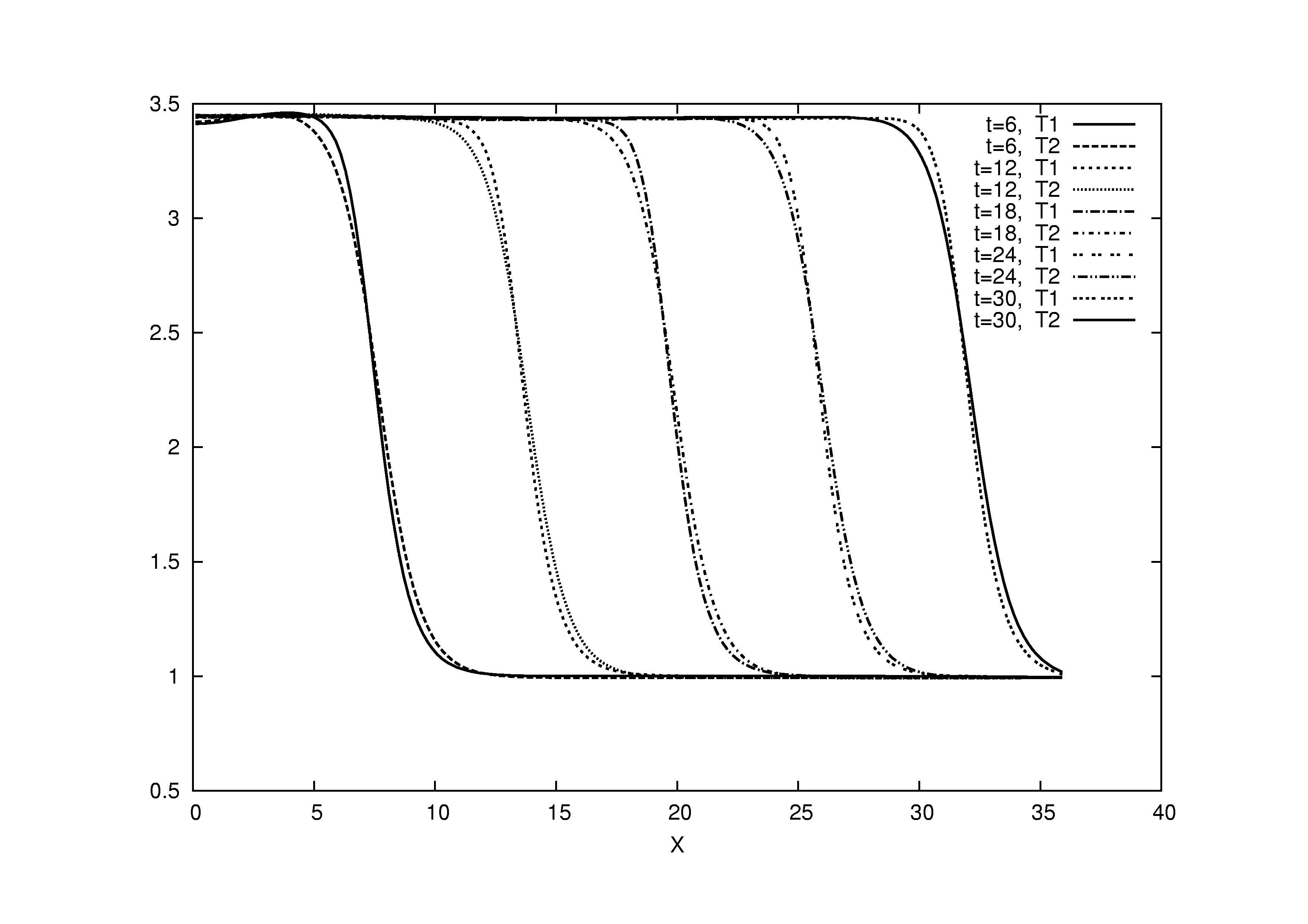
Figure 1: Mirror reflection. Profiles of temperatures of the mixture components at different times.

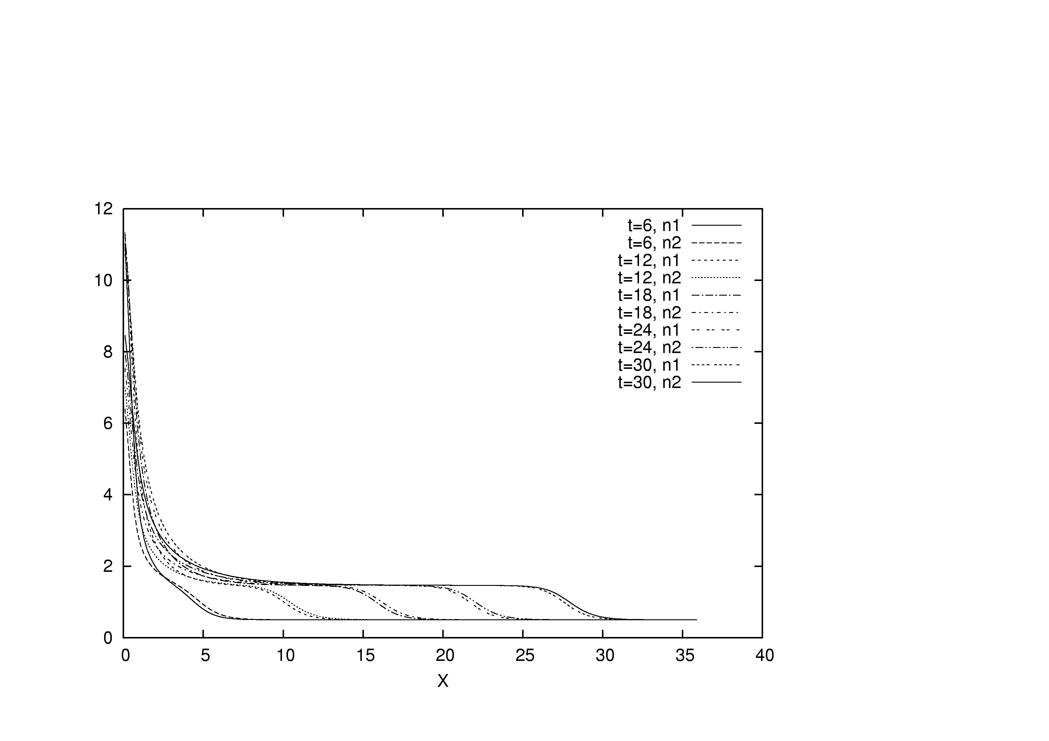
Figure 2: Diffuse reflection. Profiles of numerical densities of the mixture components at different times. Temperature of the wall is equal to 0.5.

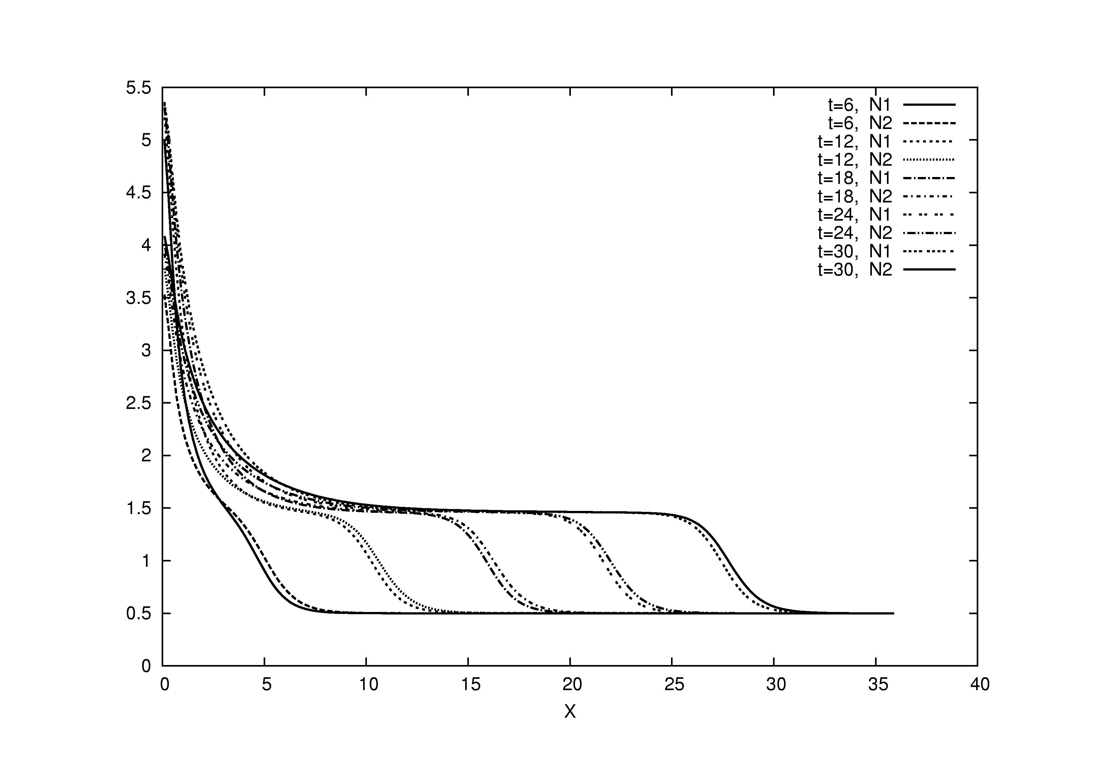
Figure 3: Diffuse reflection. Profiles of numerical densities of the mixture components at different times. Temperature of the wall is equal to 1.

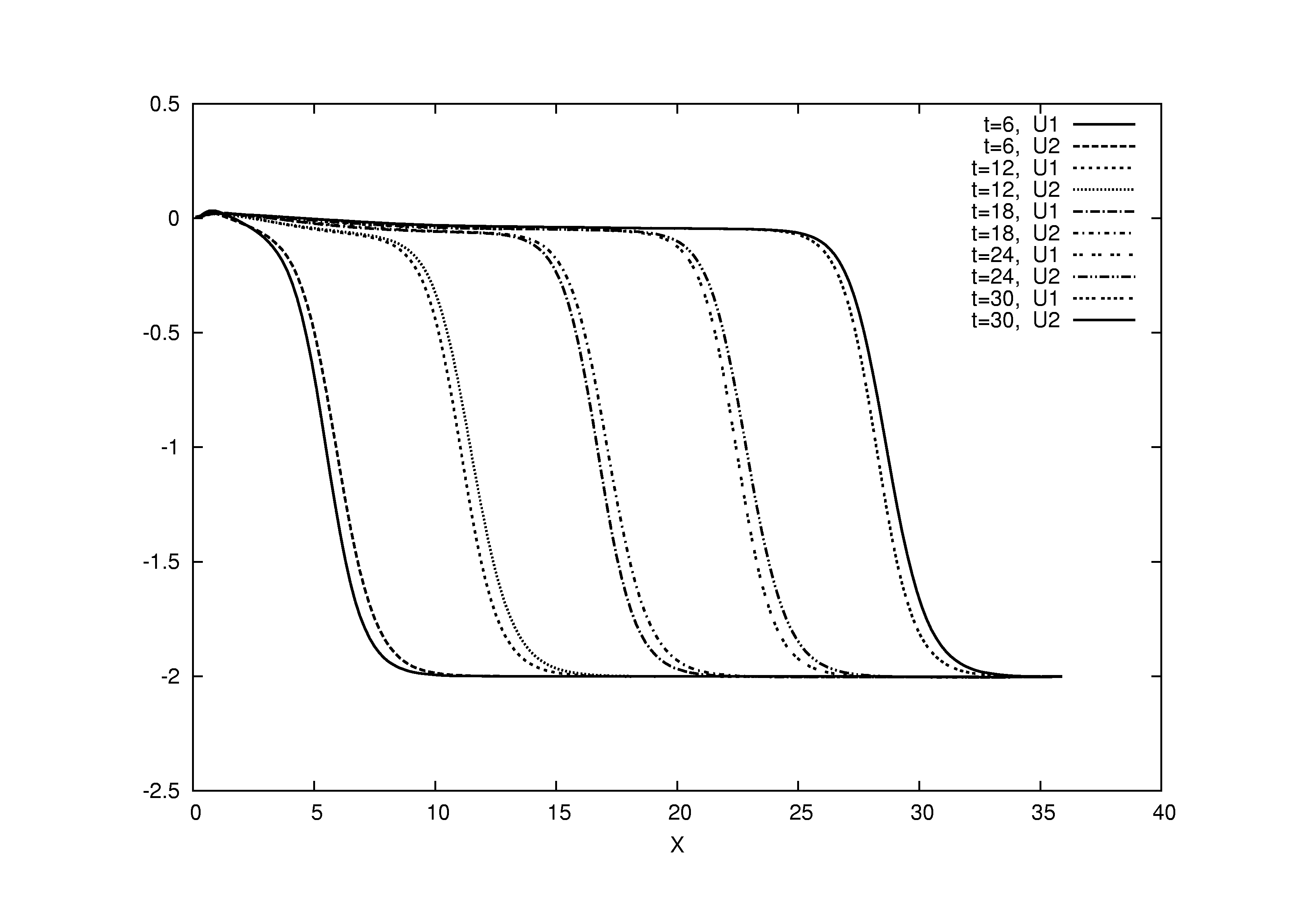
Figure 4: Diffuse reflection. Profiles of velocities of the mixture components at different times. Temperature of the wall is equal to 1.

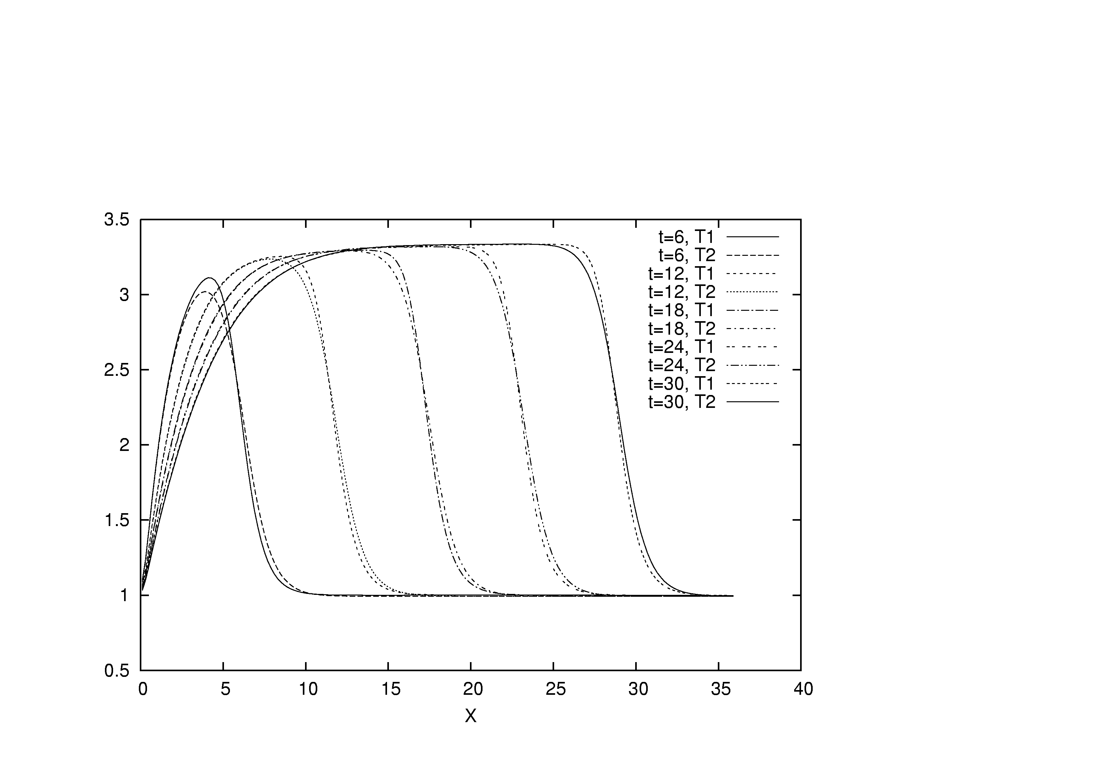
Figure 5: Diffuse reflection. Profiles of temperatures of the mixture components at different times. Temperature of the wall is equal to 1.

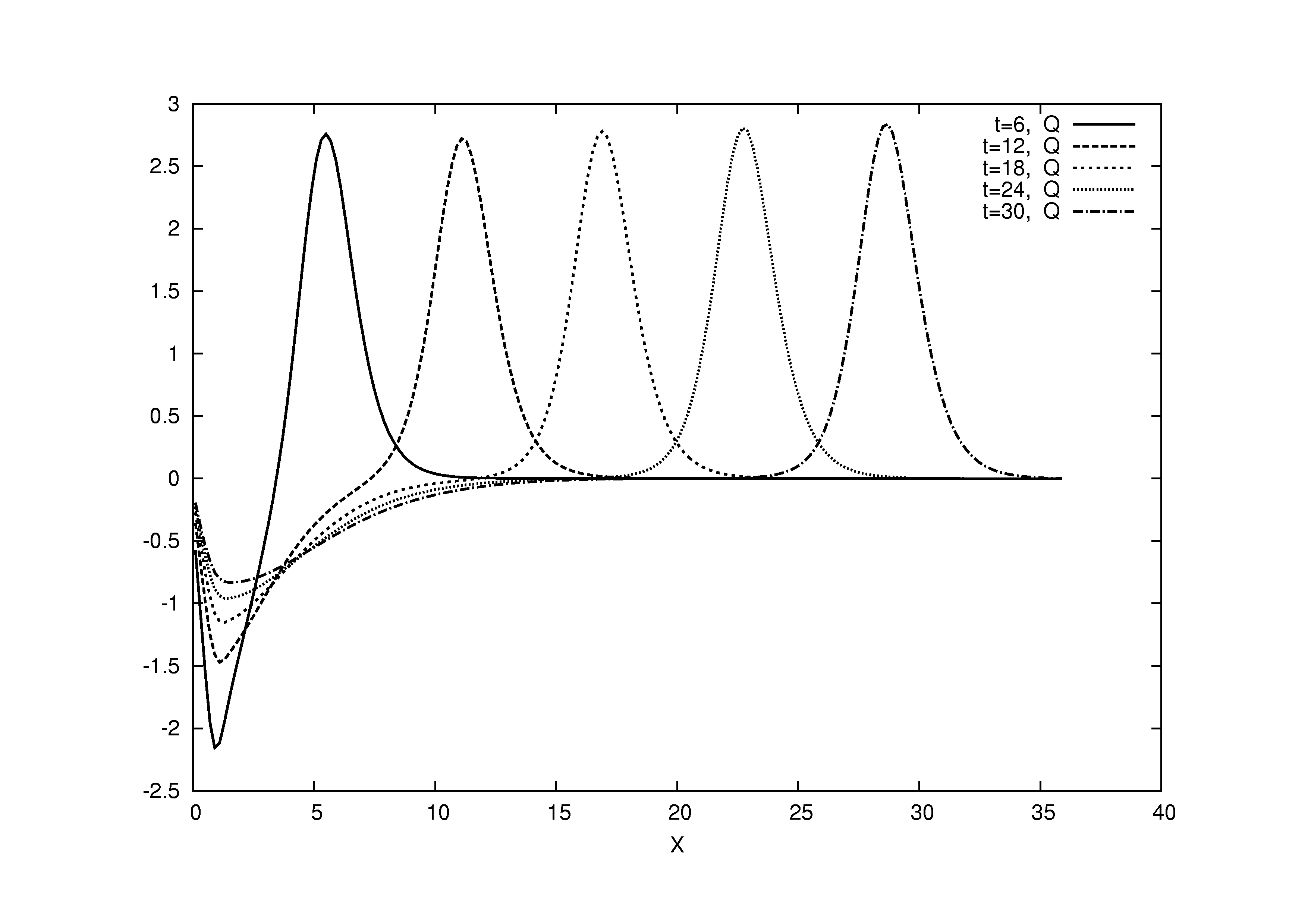
Figure 6: Diffuse reflection. Profiles of the heat flow of the gas mixture at different times. Temperature of the wall is equal to 0.5.

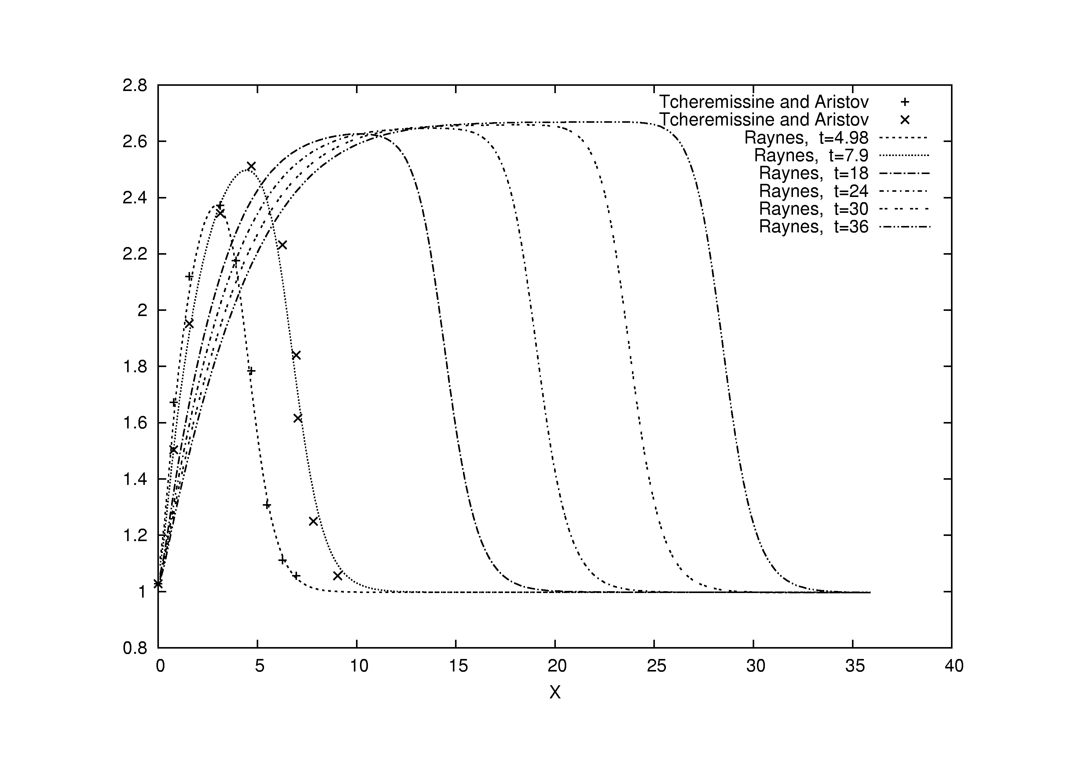
Figure 7: Comparison of results of Raines (Raynes) with the paper [3] for temperature profiles for a one-component gas.

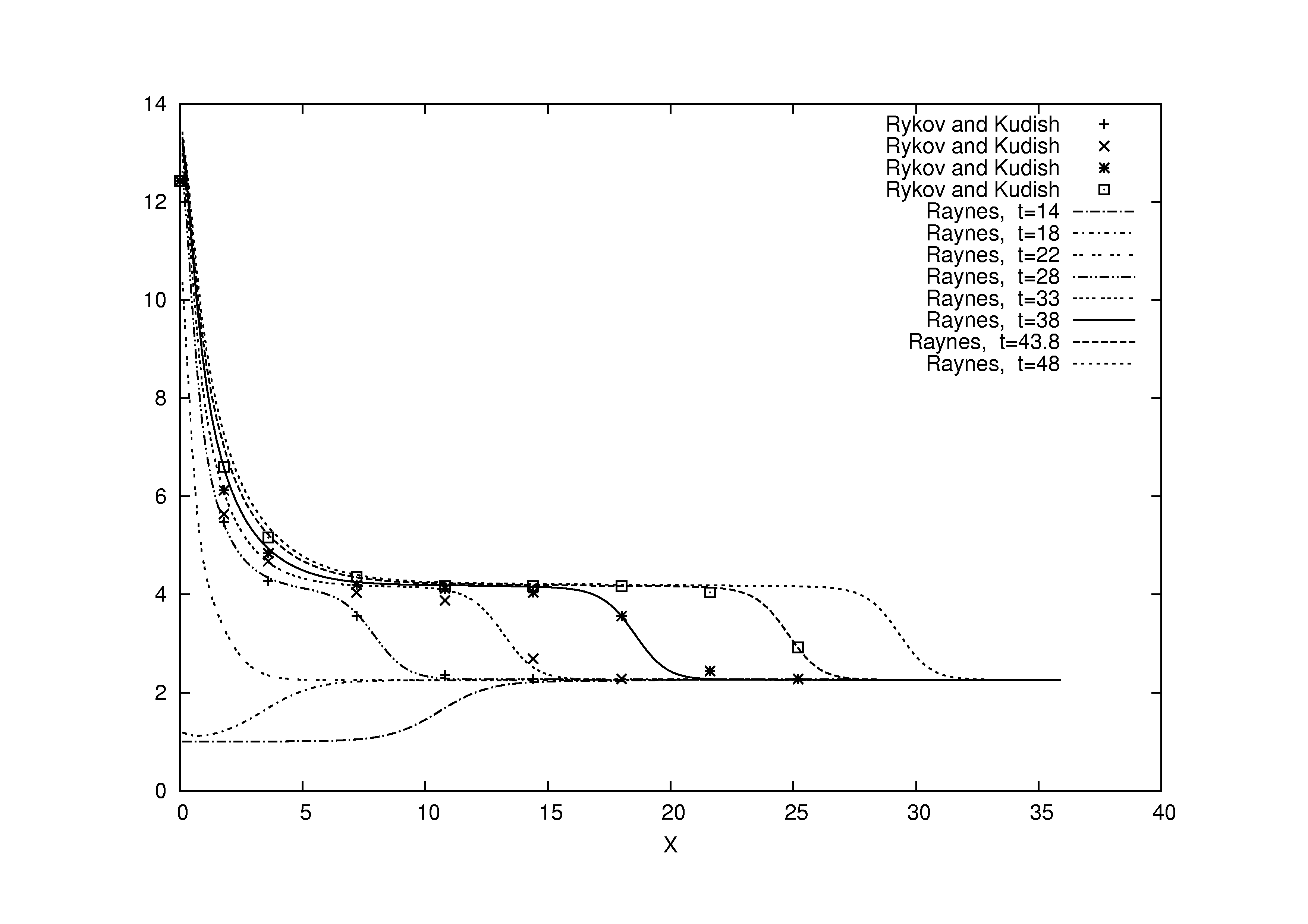
Figure 8: The problem of reflection of a shock wave from a wall. Comparison of results of Raines (Raynes) with the paper [4] for density profiles for a one-component gas.

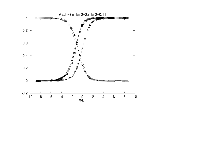
Figure 9: The problem of a shock wave in a binary gas mixture. Comparison with results of [5]. Profiles of density, velocity and temperature for the mixture.

References

• [1] Tcheremissine, F. G., 1998, Conservative evaluation of Boltzmann collision integral in discrete ordinate approximation. Comp. Math. Appl., 35, 215–221.
• [2] Raines, A. A., 2002, Study of a shock wave structure in a gas mixture on the basis of the Boltzmann equation. Eur. J. Mech. B. Fluids, 21, 599–610.
• [3] Aristov, V. V., Tcheremissine, F. G., 1978, Conservative difference scheme of discrete ordinates for solving kinetic equations by a splitting method. Direct numerical modelling of gas flows, Comp. Center of Acad. Sci. USSR, 164–171.
• [4] Kudish, I. V., Rykov, V. A., 1973, Reflection of a shock wave from a wall. J. Comp. Math. and Math. Phys., 13, No. 5, 1288–1297.
• [5] Kosuge, S., Aoki, K. and Takata, S., 2001, Shock wave structure for a binary gas mixture: finite-difference analysis of the Boltzmann equation for hard-sphere molecules, European J. Mech. B. Fluids, 20, 87–126.
Refer to caption