Abstract

The possibility is considered for the formation in optical lattices of a heterogeneous state characterized by a spontaneous mesoscopic separation of the system into the spatial regions with different atomic densities. It is shown that such states can arise, if there are repulsive interactions between atoms in different lattice sites and the filling factor is less than one-half.

Keywords: optical lattices, mesoscopic separation, heterophase states

1 Introduction

Optical lattices, loaded with cold atoms, are intensively studied, being the objects with rich properties that can be widely regulated (see, e.g., the review articles [1, 2, 3, 4]). The loaded atoms can interact with each other through short-range as well as long-range forces, such as dipolar forces [5, 6, 7].

In addition to usual insulating and delocalized equilibrium states, atoms in optical lattices can form several quasi-equilibrium and metastable states. For example, in optical lattices, there can exist metastable states with repulsively bound bosonic pairs [8], metastable states characterized by microscopic phase separation in a mixture of two bosonic species [9], quasi-equilibrium mixture of localized and itinerant bosons [10], and metastable states of atoms with dipolar interactions [11]. Double-well optical lattices can display the states with mesoscopic disorder, characterized by a heterophase mixture of mesoscopic regions with ordered and disordered atomic imbalance [12, 13]. Incorporating into the system of cold atoms impurities [14] or imposing random external fields [15] can produce glassy lattice states [16] similar to vitrified solid states of metals [17].

In the present paper, we consider the possibility of forming in an optical lattice of a heterophase state consisting of regions with different atomic densities. These regions have mesoscopic spatial sizes and are randomly distributed in space, where they are not fixed, but can appear and disappear in different places. In that sense, such a state is a dynamical heterophase mixture analogous to other heterophase states with mesoscopic phase separation, which occur in many condensed-matter systems [18, 19]. Each subregion of a competing phase is a kind of a droplet, or grain, of a denser phase inside a diluted phase. Such states are, of course, not absolutely equilibrium, but are quasi-equilibrium.

The typical linear size of a dense droplet is defined by the length $l_{cor}$, at which atoms are strongly correlated and can coherently form a single phase. This length is mesoscopic, being between the mean interatomic distance $a$ and the linear system size $L$,

$$a\ll l_{cor}\ll L\;.$$

The droplet size is rather of nanoscale, not exceeding the critical radius, after which the germ would grow, provoking a phase transition in the whole system [20]. Nanoscale nuclei of a competing phase are not equilibrium and, strictly speaking, thermodynamic notions, such as surface tension or surface energy, may be not applicable [21]. The lifetime $t_{cor}$ of a correlated subregion, forming a droplet, is also mesoscopic, being between the local equilibration time $t_{loc}$ and the observation time $t_{obs}$,

$$t_{loc}\ll t_{cor}\ll t_{obs}\;.$$

Generally speaking, the sizes and lifetimes of the droplets are of multiscale nature, being inside mesoscopic intervals, for which $l_{cor}$ and $t_{cor}$ play the role of centers [22]. To some extent, the denser subregions remind the grains arising in the process of grain turbulence [23]. An opposite situation happens in the case of a solid with cracks and pores, where there are low-density regions inside a more dense solid [24].

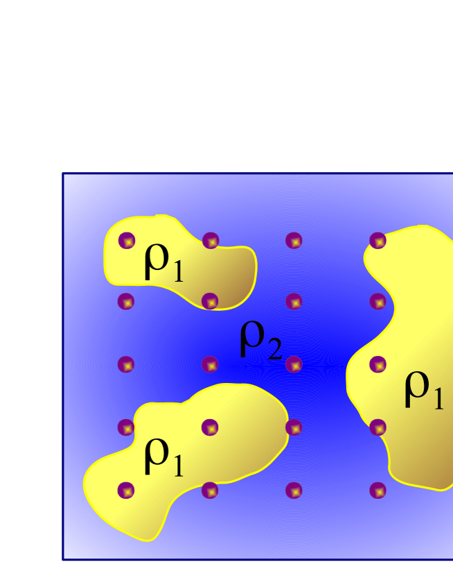
Figure 1: Snapshot of a heterophase two-density lattice system. Regions of higher density $\rho_{1}$ are randomly immersed into the matrix of lower density $\rho_{2}$, with $\rho_{1}>\rho_{2}$.

A snapshot of the heterophase two-density state is shown in Fig. 1, where the regions of higher density are randomly located inside a matrix of lower density.

The consideration of a new thermodynamic state necessarily includes the analysis of its stability. Analyzing this, we show that there exist conditions, when the two-density state in an optical lattice is really stable. These conditions, briefly speaking, require the presence of intersite atomic interactions and a low filling factor, smaller than one-half.

2 Heterophase two-density lattice state

The first step for treating a two-phase system with random subregions is the averaging over heterophase configurations [18, 19]. Keeping in mind the standard form of the Hamiltonian, after averaging over configurations, we come to the effective Hamiltonian

$$\widetilde{H}=H_{1}\bigoplus H_{2}\;,$$ (1)

consisting of two terms

$$H_{\alpha}=w_{\alpha}\int\psi_{\alpha}^{\dagger}({\bf r})\left[\hat{H}_{L}({\bf r})-\mu\right]\psi_{\alpha}({\bf r})\;d{\bf r}\;+\;\frac{w_{\alpha}^{2}}{2}\int\psi^{\dagger}_{\alpha}({\bf r})\psi^{\dagger}_{\alpha}({\bf r}^{\prime})\Phi({\bf r}-{\bf r}^{\prime})\psi_{\alpha}({\bf r}^{\prime})\psi_{\alpha}({\bf r})\;d{\bf r}d{\bf r}^{\prime}$$ (2)

representing two different phases, whose atoms are described by the field operators $\psi_{\alpha}$, with $\alpha=1,2$. Here $\hat{H}_{L}(\bf r)$ is an optical-lattice Hamiltonian and $\Phi(\bf r)$ is a pair interaction potential. The Hamiltonian is renormalized by the geometric phase probabilities

$$w_{\alpha}\equiv\frac{V_{\alpha}}{V}\qquad(V_{1}+V_{2}=V)\;,$$ (3)

where $V_{\alpha}$ is the average volume occupied by the $\alpha$ - phase and $V$ is the system volume. By this definition, the phase probability satisfies the properties

$$w_{1}+w_{2}=1\;,\qquad 0\leq w_{\alpha}\leq 1\;.$$ (4)

By assumption, the phases have different densities

$$\rho_{\alpha}\equiv\frac{N_{\alpha}}{V_{\alpha}}=\frac{1}{V}\int\langle\psi^{\dagger}_{\alpha}({\bf r})\psi_{\alpha}({\bf r})\rangle\;d{\bf r}\;,$$ (5)

in which the number of atoms in an $\alpha$ - phase is

$$N_{\alpha}=w_{\alpha}\int\langle\psi^{\dagger}_{\alpha}({\bf r})\psi_{\alpha}({\bf r})\rangle\;d{\bf r}\;.$$ (6)

Without the loss of generality, we may call the first phase more dense, so that

$$\rho_{1}>\rho_{2}\;.$$ (7)

In that sense, the densities, distinguishing the phases play the role of the order parameters.

The optical lattice prescribes the spatial periodicity of the lattice Hamiltonian $\hat{H}_{L}(\bf r)$ with respect to the lattice vectors enumerated by the index $j=1,2,\ldots,N_{L}$ running through all $N_{L}$ lattice sites. The field operators can be represented as expansions

$$\psi_{\alpha}({\bf r})=\sum_{nj}e_{j}^{\alpha}c_{nj}\varphi_{nj}({\bf r})$$ (8)

over the localized orbitals $\varphi_{nj}$. The expansion takes into account that a $j$ - site can be either occupied by an atom or free, depending on the value of the variable $e_{j}^{\alpha}=0,1$.

We assume that each lattice site can host not more than one atom, which is expressed through the unipolarity condition

$$\sum_{n}c^{\dagger}_{nj}c_{nj}=1\;,\qquad c_{mj}^{\dagger}c_{nj}^{\dagger}=0\;.$$ (9)

Substituting expansion (8) into Hamiltonian (2) yields two types of terms, with respect to the site indices $i$ and $j$. The terms, describing atomic interactions, define the effective time $t_{osc}$ of atomic oscillations in the vicinity of a given site. The other type of the terms is responsible for the hopping of atoms between the lattice sites, which can be characterized by a hopping time $t_{hop}$. The observation time has to be much longer than the hopping time, so that various phase configurations could be realized in the system, thus, justifying the averaging over these configurations. The relation between $t_{osc}$ and $t_{hop}$ describes whether the system is in an insulating or delocalized state. When $t_{osc}$ is much shorter than $t_{hop}$, the atoms are well localized. This implies that the interaction terms are much larger than the hopping terms, responsible for atom hopping. In what follows, we assume that atoms are sufficiently well localized, so that the hopping terms are small, as compared to the interaction terms. Then the diagonal approximation can be employed corresponding to the following form of the matrix elements:

$$\langle mi\;|\;\hat{H}_{L}\;|\;nj\rangle=\delta_{mn}\delta_{ij}E_{0}\;,\qquad\langle mi,nj\;|\;\Phi\;|\;m^{\prime}i^{\prime},n^{\prime}j^{\prime}\rangle=\delta_{mm^{\prime}}\delta_{nn^{\prime}}\delta_{ii^{\prime}}\delta_{jj^{\prime}}\Phi_{ij}\;.$$ (10)

The constant term $E_{0}$ can be incorporated into the chemical potential. In this way, Hamiltonain (2) reduces to the form

$$H_{\alpha}=-w_{\alpha}\mu\sum_{j=1}^{N_{L}}e_{j}^{\alpha}\;+\;\frac{1}{2}\;w_{\alpha}^{2}\sum_{i\neq j}^{N_{L}}\Phi_{ij}e_{i}^{\alpha}e_{j}^{\alpha}\;.$$ (11)

Using the canonical transformation

$$e_{j}^{\alpha}=\frac{1}{2}+S_{j}^{z}\qquad\left(e_{j}^{\alpha}=0,1\right)\;,\qquad\qquad S_{j}^{z}=e_{j}^{\alpha}-\;\frac{1}{2}\qquad\left(S_{j}^{z}=\pm\frac{1}{2}\right)\;,$$ (12)

we come to the pseudospin representation

$$H_{\alpha}=\frac{N_{L}}{8}\;\left(w_{\alpha}^{2}\Phi-4w_{\alpha}\mu\right)+\frac{1}{2}\;\left(w_{\alpha}^{2}\Phi-2w_{\alpha}\mu\right)\sum_{j=1}^{N_{L}}S_{j}^{z}\;+\;\frac{w_{\alpha}^{2}}{2}\sum_{i\neq j}^{N_{L}}\Phi_{ij}S_{i}^{z}S_{j}^{z}\;,$$ (13)

where

$$\Phi\equiv\frac{1}{N_{L}}\sum_{i\neq j}^{N_{L}}\Phi_{ij}=\sum_{j(\neq i)}^{N_{L}}\Phi_{ij}\;.$$ (14)

Then we resort to the mean-field approximation resulting in the Hamiltonian

$$H_{\alpha}=\frac{N_{L}}{8}\;\left[w_{\alpha}^{2}\Phi\left(1-s_{\alpha}^{2}\right)-4w_{\alpha}\mu\right]+\frac{1}{2}\;\left[w_{\alpha}^{2}\Phi\left(1+s_{\alpha}\right)-2w_{\alpha}\mu\right]\sum_{j=1}^{N_{L}}S_{j}^{z}\;,$$ (15)

in which the notation

$$s_{\alpha}\equiv 2\langle S_{j}^{z}\rangle_{\alpha}=\frac{2}{N_{L}}\sum_{j=1}^{N_{L}}\;\langle S_{j}^{z}\rangle_{\alpha}$$ (16)

is introduced. The average $\langle S_{j}^{z}\rangle_{\alpha}$ is taken with respect to Hamiltonain (15). Quantity (16) can be calculated either directly or by minimizing the thermodynamic grand potential

$$\frac{\Omega}{N_{L}}=\frac{1}{8}\sum_{\alpha}w_{\alpha}^{2}\Phi(1-s_{\alpha}^{2})-\;\frac{1}{2}\;\mu-2T\ln 2-T\sum_{\alpha}\ln\;\cosh\left[\frac{w_{\alpha}^{2}\Phi(1+s_{\alpha})-2w_{\alpha}\mu}{4T}\right]\;,$$ (17)

which gives

$$s_{\alpha}=\tanh\left[\frac{2w_{\alpha}\mu-w_{\alpha}^{2}\Phi(1+s_{\alpha})}{4T}\right]\;.$$ (18)

Minimizing the grand potential (17) with respect to the phase probability, under the normalization condition (4), we set

$$w\equiv w_{1}\;,\qquad w_{2}=1-w\;.$$ (19)

The minimization yields the equation

$$\sum_{\alpha}\left[2\mu s_{\alpha}-w_{\alpha}\Phi(1+s_{\alpha})^{2}\right]\;\frac{\partial w_{\alpha}}{\partial w}=0\;,$$

from which we may express the chemical potential

$$\mu=\frac{w_{1}(1+s_{1})^{2}-w_{2}(1+s_{2})^{2}}{2(s_{1}-s_{2})}\;\Phi\;.$$ (20)

An important quantity is the filling factor

$$\nu\equiv\frac{N}{N_{L}}\qquad(N=N_{1}+N_{2})\;.$$ (21)

Representing the particle number (6) as

$$N_{\alpha}=\frac{N_{L}}{2}\;w_{\alpha}(1+s_{\alpha})\;,$$ (22)

we have the filling factor

$$\nu=\frac{1}{2}\sum_{\alpha}w_{\alpha}(1+s_{\alpha})\;.$$ (23)

Inverting this with respect to the phase probability of the dense phase, we get

$$w_{1}=\frac{2\nu-1-s_{2}}{s_{1}-s_{2}}\;.$$ (24)

It is convenient to introduce the dimensionless quantity

$$x_{\alpha}\equiv\frac{1}{N_{L}}\sum_{j=1}^{N_{L}}\;\langle e_{j}^{\alpha}\rangle_{\alpha}\;,$$ (25)

playing the role of a dimensionless order parameter. For the dense and diluted phases, we write

$$x\equiv x_{1}=\frac{1}{2}\;(1+s_{1})\;,\qquad y\equiv x_{2}=\frac{1}{2}\;(1+s_{2})\;,$$ (26)

respectively. The density of the $\alpha$-phase reads as

$$\rho_{\alpha}\equiv\frac{N_{\alpha}}{V_{\alpha}}=\frac{N_{L}}{V}\;x_{\alpha}\;,$$ (27)

which shows why quantities (25) play the role of dimensionless order parameters. Due to inequality (7), we have the condition

$$x>y\;,$$ (28)

distinguishing the phases with respect to their densities.

The filling factor (23) can be written as

$$\nu=w_{1}x+w_{2}y\;.$$ (29)

Because of condition (28), the relation

$$y\leq\nu\leq x$$ (30)

holds true.

Using notation (26) reduces the chemical potential (20) to the form

$$\mu=\frac{w_{1}x^{2}-w_{2}y^{2}}{x-y}\;\Phi\;.$$ (31)

From Eq. (24), we find the phase probabilities

$$w_{1}=\frac{\nu-y}{x-y}\;,\qquad w_{2}=\frac{x-\nu}{x-y}\;.$$ (32)

The sign

$$\sigma\equiv\frac{\Phi}{|\Phi|}={\rm sgn}\Phi$$ (33)

of the effective interaction (14), for a while, is arbitrary. Measuring temperature in units of $|\Phi|$, for the order-parameters (26), we get

$$2x=1+\sigma\tanh\left[\frac{w_{1}y(w_{1}x-w_{2}y)}{2T(x-y)}\right]\;,$$

$$2y=1+\sigma\tanh\left[\frac{w_{2}x(w_{1}x-w_{2}y)}{2T(x-y)}\right]\;.$$ (34)

Thermodynamic quantities can be found from the free energy, for which we define the dimensionless quantity

$$F\equiv\frac{\Omega+\mu N}{N_{L}|\Phi|}=\frac{\sigma}{2}\left[w_{1}^{2}x(1-x)+w_{2}^{2}y(1-y)\right]+\frac{T}{2}\ln[x(1-x)y(1-y)]+\frac{\mu}{|\Phi|}\left(\nu-\;\frac{1}{2}\right)\;.$$ (35)

3 Stability of heterophase two-density state

First of all, we recall that to be stable a heterophase system has to satisfy the necessary heterophase stability condition

$$\left(\left\langle\frac{\partial^{2}H}{\partial w^{2}}\right\rangle\right)>0\;,$$ (36)

which follows from the minimization of the grand potential [18, 19]. This leads to the inequality

$$\left\langle\frac{\partial^{2}H}{\partial w^{2}}\right\rangle=N_{L}\Phi(x^{2}+y^{2})>0\;,$$ (37)

from which it is clear that the effective interaction (14) has to be effectively repulsive, so that

$$\Phi>0\;.$$ (38)

An effectively attractive interaction does not allow for the formation of a stable heterophase system.

Additionally, the system should be thermodynamically stable, implying that the specific heat

$$C_{V}=-T\left(\frac{\partial^{2}F}{\partial T^{2}}\right)_{V}$$ (39)

and the isothermal compressibility

$$\kappa_{T}=\frac{1}{\nu^{2}}\;\left(\frac{\partial^{2}F}{\partial\nu^{2}}\right)^{-1}_{T}$$ (40)

be non-negative and finite [25],

$$0\leq C_{V}<\infty\;,\qquad 0\leq\kappa_{T}<\infty\;.$$ (41)

In what follows, we again measure temperature in units of $\Phi$. Keeping in mind that we need to consider only repulsive atomic interactions, we have to solve the system of equations for the order parameter of the dense phase

$$2x=1+\tanh\left\{\frac{wy[wx-(1-w)y]}{2T(x-y)}\right\}\;,$$ (42)

the order parameter of the rarefied phase

$$2y=1+\tanh\left\{\frac{(1-w)x[wx-(1-w)y]}{2T(x-y)}\right\}\;,$$ (43)

and the probability of the dense phase

$$w=\frac{\nu-y}{x-y}\;.$$ (44)

The corresponding solutions define the free energy

$$F=\frac{1}{2}\left[w^{2}x(1-x)+(1-w)^{2}y(1-y)\right]+\frac{1}{2}\;T\ln[x(1-x)y(1-y)]\;+$$

$$+\;\left(\nu-\;\frac{1}{2}\right)\;\frac{wx^{2}-(1-w)y^{2}}{x-y}\;,$$ (45)

from where the specific heat and compressibility can be calculated.

Solving Eqs. (42), (43), and (44), we are looking for the probability in the interval $0\leq w\leq 1$ and for the order parameters satisfying the inequalities

$$0\leq y\leq\nu\leq x\leq 1\;.$$

Numerical investigation shows that the heterophase system can be stable only for small filling factors,

$$0<\nu<\frac{1}{2}\;.$$

For larger filling factors, compressibility (40) becomes negative, although specific heat (39) is always positive.

Solutions to Eqs. (42) to (44) exist in the temperature interval $[T_{n},T_{n}^{*}]$. These temperatures can be called the lower nucleation temperature and upper nucleation temperature. The lower nucleation temperature $T_{n}$ is found numerically, being zero for $\nu<0.32$. The upper nucleation temperature $T_{n}^{*}$ is defined by the conditions

$$w(T_{n}^{*})=0\;,\qquad x(T_{n}^{*})=\frac{1}{2}\;,\qquad y(T_{n}^{*})=\nu\;,$$

which yields

$$T_{n}^{*}=\frac{\nu}{(1-2\nu)\ln(\frac{1}{\nu}-1)}\;.$$

When $\nu\rightarrow 1/2$, then both $T_{n}$ and $T_{n}^{*}$ tend to infinity. Table 1 gives the values of $T_{n}$ and $T_{n}^{*}$ in the allowed interval of $0<\nu<1/2$.

Figure 2 presents the behavior of solutions as functions of temperature for different filling factors and Fig. 3, as functions of the filling factor for different temperatures. Specific heat (39) and compressibility (40) are positive. For illustration, $C_{V}$, as a function of temperature, is shown in Fig. 4.

4 Comparison with pure single-density state

The heterophase two-density state should be compared with the pure single-phase state, when $w\equiv 1$. Then the grand potential is

$$\frac{\Omega_{1}}{N_{L}}=\frac{1}{8}\;\Phi(1-s^{2})\;-\;\frac{1}{2}\;\mu_{1}\;-\;T\ln 2\;-\;T\ln\;\cosh\left[\frac{\Phi(1+s)-2\mu_{1}}{4T}\right]\;,$$ (46)

where

$$s=\tanh\left[\frac{2\mu_{1}-\Phi(1+s)}{4T}\right]\;.$$ (47)

The filling factor reads as

$$\nu\equiv\frac{N}{N_{L}}=\frac{1}{2}\;(1+s)\;.$$ (48)

From Eqs. (47) and (48), we have

$$2\nu=1+\tanh\left(\frac{\mu_{1}-\nu\Phi}{2T}\right)\;,$$

which results in the chemical potential

$$\mu_{1}=\nu\Phi+T\ln\frac{\nu}{1-\nu}\;.$$ (49)

For the dimensionless free energy, we get

$$F_{1}\equiv\frac{\Omega_{1}+\mu_{1}N}{N_{L}|\Phi|}=\frac{1}{2}\;\sigma\nu^{2}+T[\nu\ln\nu+(1-\nu)\ln(1-\nu)]\;.$$ (50)

This shows that, for the pure phase, the specific heat is zero, $C_{V}=0$. And for the compressibility, we find

$$\kappa_{1}=\frac{1-\nu}{\nu[\sigma\nu(1-\nu)+T]}\;.$$

The latter is positive, provided that

$$T>-\sigma\nu(1-\nu)\;.$$

In the case of repulsive interactions, when $\sigma=1$, the pure phase can exist at all temperatures. But for attractive interactions, when $\sigma=-1$, the system is stable only for sufficiently high temperatures, such that $T>\nu(1-\nu)$.

Comparing the free energy (45) of the heterophase two-density state with the free energy (50) of the pure single-density state, we find that, in all those cases, when the heterophase state exists, $F<F_{1}$. This is shown in Fig. 5 for repulsive interactions. Therefore, in the temperature region $T_{n}<T<T_{n}^{*}$, the heterophase state is stable, while the pure state is metastable.

5 Conclusion

We have considered the possibility of the formation in optical lattices of a heterogeneous state characterized by a spontaneous mesoscopic separation of the system into the spatial regions with two different atomic densities, one being more dense than the other. We show that such states can really occur, provided that atomic interactions between atoms in different lattice sites are repulsive and the filling factor is less than one-half. The heterophase state is stable in the temperature region between the lower, $T_{n}$, and upper, $T_{n}^{*}$, nucleation temperatures.

Figure 1. Snapshot of a heterophase two-density lattice system. Regions of higher density $\rho_{1}$ are randomly immersed into the matrix of lower density $\rho_{2}$, with $\rho_{1}>\rho_{2}$.

Figure 2. Solutions as functions of dimensionless temperature $T$ for different filling factors: (a) order parameters $x$ (solid line) and $y$ (dashed line) for $\nu=0.1$ (line 1), $\nu=0.2$ (line 2), $\nu=0.3$ (line 3), and $\nu=0.32874$ (line 4); (b) dense-phase probability $w$ for the same filling factors and enumeration as above; (c) order parameters $x$ (solid line) and $y$ (dashed line) for $\nu=0.33$ (line 1), $\nu=0.4$ (line 2), and $\nu=0.45$ (line 3); (d) dense-phase probability $w$ for the same filling factors and enumeration as in (c).

Figure 3. Order parameters $x$ (solid line) and $y$ (dashed line) and the dense-phase probability $w$ (dashed-dotted line) as functions of filling factor $\nu$ for different temperatures: (a) $T=0.01$; (b) $T=0.5$.

Figure 4. Specific heat as function of temperature for different filling factors: (a) $\nu=0.1$ (line 1), $\nu=0.2$ (line 2), $\nu=0.3$ (line 3), and $\nu=0.32874$ (line 4); (b) $\nu=0.33$ (line 1), $\nu=0.4$ (line 2), and $\nu=0.45$ (line 3).

Figure 5. Free energy $F$ (solid line) of the heterophase state, compared to the free energy $F_{1}$ (dashed line) of the pure state, for varying temperature and different filling factors: (a) $\nu=0.3$; (b) $\nu=0.45$.

Table Caption

Table 1. Lower and upper temperatures defining the existence interval of the optical lattice with heterogeneous densities.

         

         

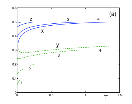
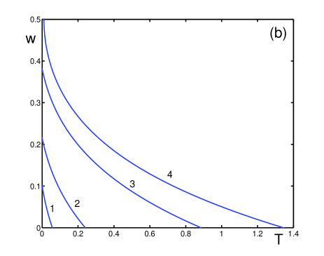
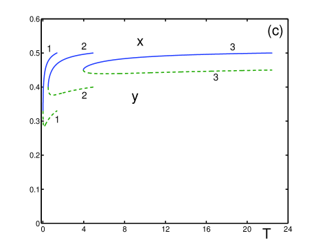
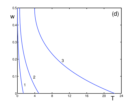
Figure 2: Solutions as functions of dimensionless temperature $T$ for different filling factors: (a) order parameters $x$ (solid line) and $y$ (dashed line) for $\nu=0.1$ (line 1), $\nu=0.2$ (line 2), $\nu=0.3$ (line 3), and $\nu=0.32874$ (line 4); (b) dense-phase probability $w$ for the same filling factors and enumeration as above; (c) order parameters $x$ (solid line) and $y$ (dashed line) for $\nu=0.33$ (line 1), $\nu=0.4$ (line 2), and $\nu=0.45$ (line 3); (d) dense-phase probability $w$ for the same filling factors and enumeration as in (c).

         

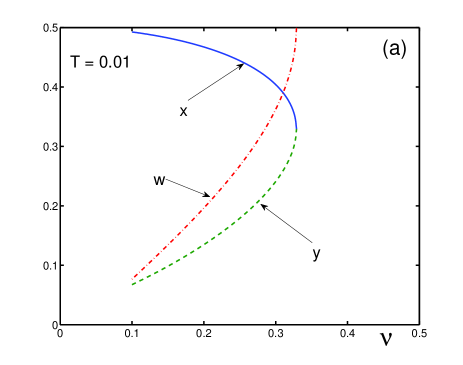
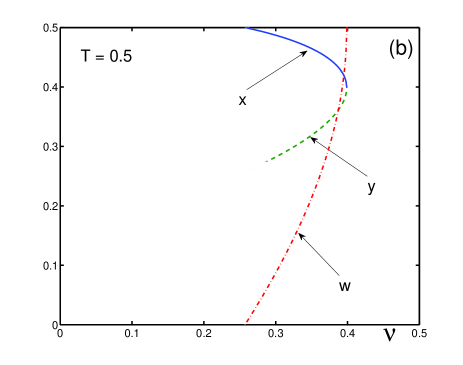
Figure 3: Order parameters $x$ (solid line) and $y$ (dashed line) and the dense-phase probability $w$ (dashed-dotted line) as functions of filling factor $\nu$ for different temperatures: (a) $T=0.01$; (b) $T=0.5$.

         

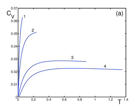
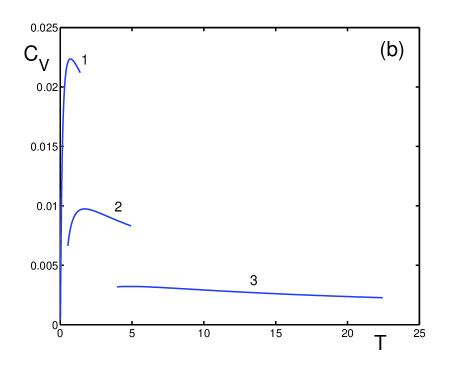
Figure 4: Specific heat as function of temperature for different filling factors: (a) $\nu=0.1$ (line 1), $\nu=0.2$ (line 2), $\nu=0.3$ (line 3), and $\nu=0.32874$ (line 4); (b) $\nu=0.33$ (line 1), $\nu=0.4$ (line 2), and $\nu=0.45$ (line 3).

         

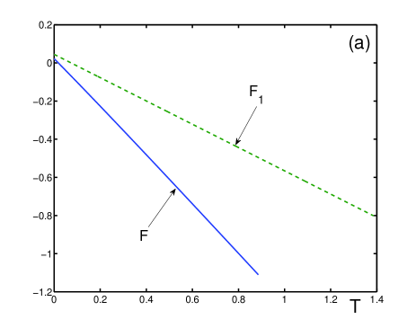
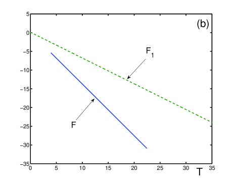
Figure 5: Free energy $F$ (solid line) of the heterophase state, compared to the free energy $F_{1}$ (dashed line) of the pure state, for varying temperature and different filling factors: (a) $\nu=0.3$; (b) $\nu=0.45$.

References

- [1] Morsch O and Oberthaler M 2006 Rev. Mod. Phys. 78 179
- [2] Moseley C, Fialko O and Ziegler K 2008 Ann. Phys. (Berlin) 17 561
- [3] Bloch I, Dalibard J and Zwerger W 2008 Rev. Mod. Phys. 80 885
- [4] Yukalov V I 2009 Laser Phys. 19 1
- [5] Griesmaier A 2007 J. Phys. B 40 91
- [6] Baranov M A 2008 Phys. Rep. 464 71
- [7] Baranov M A, Dalmonte M, Pupillo G and Zoller P 2012 Chem. Rev. 112 5012
- [8] Winkler K, Thalhammer G, Grimm R, Denschlag J H, Daley A J, Kantian A, Büchler H P and Zoller P 2006 Nature 441 853
- [9] Roscilde T and Cirac J I 2007 Phys. Rev. Lett. 98 190402
- [10] Yukalov V I, Rakhimov A and Mardonov S 2011 Laser Phys. 21 264
- [11] Santos L 2013 in Many-Body Physics with Ultracold Atoms eds Salomon C, Shlyapnikov G and Cugliandolo L F 2013 (Oxford: Oxford University)
- [12] Yukalov V I and Yukalova E P 2011 Laser Phys. 21 1448
- [13] Yukalov V I and Yukalova E P 2012 Laser Phys. 22 1070
- [14] Massignan P, Zaccanti M and Bruun G M 2014 Rep. Prog. Phys. 77 034401
- [15] Sanchez-Palencia L, Clément D, Lugan P, Bouyer P and Aspect A 2008 New J. Phys. 10 045019
- [16] Gurarie V, Pollet L, Prokofiev N V, Svistunov B V and Troyer M 2009 Phys. Rev. B 80 214519
- [17] Johnson W L and Fecht H J 1988 J. Less-Common Metals 145 63
- [18] Yukalov V I 1991 Phys. Rep. 208 395
- [19] Yukalov V I 2003 Int. J. Mod. Phys. B 17 2333
- [20] Bakai A S 2013 Polycluster Amorphous Solids (Kharkov: Sinteks)
- [21] Kharlamov G V, Onischuk A A, Vosel S V and Purtov P A 2012 J. Phys. Conf. Ser. 393 012006
- [22] Yukalov V I and Yukalova E P 2012 J. Phys. Chem. B 116 8435
- [23] Yukalov V I, Novikov A N and Bagnato V S 2014 Laser Phys. Lett. 11 095501
- [24] Yukalov V I 1989 Int. J. Mod. Phys. B 3 311
- [25] Yukalov V I 2013 Laser Phys. 23 062001
Figure Captions