Chemical Abundances of the Highly Obscured Galactic Globular Clusters 2MASS GC02 and Mercer 5

Abstract

We present the first high spectral resolution abundance analysis of two newly discovered Galactic globular clusters, namely Mercer 5 and 2MASS GC02 residing in regions of high interstellar reddening in the direction of the Galactic center. The data were acquired with the Phoenix high-resolution near-infrared echelle spectrograph at Gemini South (R $\sim 50000$) in the 15500.0 - 15575.0 spectral region. Iron, Oxygen, Silicon, Titanium and Nickel abundances were derived for two red giant stars, in each cluster, by comparing the entire observed spectrum with a grid of synthetic spectra generated with MOOG. We found [Fe/H] values of $-0.86\pm 0.12$ and $-1.08\pm 0.13$ for Mercer 5 and 2MASS GC02 respectively. The [O/Fe], [Si/Fe] and [Ti/Fe] ratios of the measured stars of Mercer 5 follow the general trend of both bulge field and cluster stars at this metallicity, and are enhanced by $\geq+$ 0.3. The 2MASS GC02 stars have relatively lower ratios, but still compatible with other bulge clusters. Based on metallicity and abundance patterns of both objects we conclude that these are typical bulge globular clusters.

1 Introduction

The properties of globular clusters and of their stellar populations provide fundamental information on the environment where galaxies formed, on the Galactic formation process, and are a basic ingredient for the understanding of the stellar populations in the external galaxies. Moreover, the properties of globular clusters are deeply connected with the history of their host galaxy. We believe today that galaxy collisions, galaxy cannibalism, as well as galaxy mergers leave their imprint on the globular cluster population of any given galaxy. Thus, when investigating globular clusters we hope to be able to use them as an acid test for our understanding of the formation and evolution of galaxies. The Galactic bulge is particularly important in the context of galaxy formation, as it is the only bulge that can be resolved into stars down to the bottom of the main sequence, and for which chemical abundances can be obtained with high-resolution spectra. Determinations of detailed chemical compositions are key data for studies of the origin and evolution of stellar populations, since they carry characteristic signatures of the objects that enrich the interstellar gas. The Galactic bulge globular clusters are relatively poorly understood stellar systems. The number of bulge globular cluster stars for which detailed chemical abundance information is available is considerably smaller compared to stars in halo clusters. Moreover, the advent of the new generation extensive surveys such as SDSS (Abazajian et al., 2009), 2MASS (Skrutskie et al., 2006), GLIMPSE (Benjamin et al., 2003), VISTA Variables in the Via Lactea (VVV) Public Survey (Minniti et al., 2010; Saito et al., 2012) yielded detection of several new Galactic Globular Clusters (GGCs). The December 2010 compilation of the Harris (1996) catalog included seven new GGCs not present in the February 2003 version, but several more cluster candidates have been proposed in the last years: SDSSJ1257+3419 (Sakamoto & Hasegawa, 2006), FSR 584 (Bica et al., 2007), FSR 1767 (Bonatto et al., 2007), FSR 190 (Froebrich et al., 2008a), Pfleiderer 2 (Ortolani et al., 2009), VVV CL001 (Minniti et al., 2011), Mercer 5 (Longmore et al., 2011), VVV CL002 (Moni Bidin et al., 2011) and Kronberger 49 (Ortolani et al., 2012). Thus, detailed investigation of these newly discovered members of the globular cluster family can contribute significantly to the global understanding of the whole system. In this study we report the results of our high-resolution Phoenix spectroscopy of selected red giant stars of two newly-discovered globular clusters: 2MASS GC02 and Mercer 5, projected in the bulge area of the Galaxy. The globular cluster 2MASS GC02 was reported by Hurt et al. (2000) and was detected within the Two Micron All Sky Survey (2MASS). Later on Borissova et al. (2007) obtained deep infrared images and low-resolution K-band spectra. Based on the analysis of the J-Ks versus Ks color-magnitude diagram and spectroscopically derived metallicities and radial velocities of 15 stars they concluded that the cluster is moderately metal-rich ([Fe/H]=-1.1) and has a relatively high radial velocity. Its horizontal branch appears to be predominantly red, though the photometry can not rule out presence of a blue component as seen in NGC 6388 and NGC 6441. Comparison with the existing kinematic and abundance information for the GGCs indicates that 2MASS GC02 most probably belongs to the bulge sub-population, although inner halo association can not be ruled out. Recently, Alonso-García et al. (2014) discovered 29 new variables inside the tidal radius of 2MASS GC02, using the Vista varaibles in the Via Lactea (VVV) ESO Large Public Survey. Eight of these variables are classified as RR Lyr stars. Using these newly discovered RR Lyrae stars, they found that the extinction towards the cluster is highly differential, and seems to follow a non-standard law, thus putting the cluster closer to the galactic center (calculated distance of RGc = 2.2 Kpc).

The dust-obscured Galactic star cluster Mercer 5 was investigated by Longmore et al. (2011). The analysis of the near-infrared photometry from the United Kingdom Infrared Digital Sky Survey (UKIDSS) and the SofI/NTT near-IR spectroscopy, indicate that the object almost certainly is a Galactic Globular Cluster, located at the edge of the Galactic bulge. The cluster suffers strong and variable extinction, located at a distance of approximately 5.5 kpc and is also moderately metal-rich ([Fe/H]=-1.0).

2 Data, Reduction and Analysis

Relevant information about our target clusters is presented in Table 1. Note that Mercer 5 is a newly discovered cluster (Mercer et al., 2005), still not included in the online version of the Harris (1996) catalog (2010 edition). Both globular clusters targeted for observations are located at low Galactic latitude, close to the plane of the Milky Way, in regions of high interstellar reddening (see Figure 1). Hence Phoenix high-resolution near-infrared echelle spectrograph (Hinkle et al., 1998) mounted at Gemini South 8-m telescope was a natural choice for the observations. The combination of large telescope aperture and high spectral resolution is crucial for accurate abundance determination, considering the apparent magnitudes of the individual red giants in our sample. More specifically, the data reported in Table 1 are taken from Longmore et al. (2011) (Mercer 5) and Borissova et al. (2007) (2MASS GC02). The fundamental parameters of both clusters are calculated using the technique outlined in Ferraro et al. (2006); Valenti et al. (2005) and Valenti et al. (2007), which allows to determine the reddening, distance modulus, and a global photometric metallicity of a globular cluster from its near-infrared CMD. In this case the RGB and HB clump calibrations were used. The targeted wavelength range was selected based on the line list published by Ryde et al. (2010) and covers a variety of Iron and $\alpha$–elements metal lines. It also has the advantage of being devoid of bright OH airglow lines, which aids the analysis of faint spectral features. The Phoenix configuration that was used is presented in Table 2. Note that the spectral coverage provided by Phoenix is limited by the size of the science array and is much smaller than the bandwidth of the H6420 order-sorting filter.

Table 1: Information about the targeted clusters

ID	RA	DEC	l	b	D	$E(J-K)$	$(m-M)_{0}$	Ref.
	hh:mm:ss	dd:mm:ss	deg.	deg.	arcmin.	mag.	mag.
(1)	(2)	(3)	(4)	(5)	(6)	(7)	(8)	(9)
2M GC02	18:09:37	-20:46:44	9.78	-0.62	$1.9\pm 0.2$	$3.0\pm 0.1$	$13.54\pm 0.15$	$a,b$
Mercer 5	18:23:19	-13:40:02	17.59	-0.11	0.60	$2.1\pm 0.7$	$14.29^{(1)}$	$c,d$
Notes: Column (1) is the cluster ID, followed by the equatorial coordinates of the ob-
ject (columns (2) and (3)). The Galactic coordinates are presented in columns
(4) and (5). Column (6) shows the apparent diameter of the cluster, followed by
an estimate of the color excess E(J-K) in column (7). The distance mo-
dulus to the object is listed in column (8), followed by the list of the references
to the various sources of information used in the table.
(1) The maximum $(m-M)_{0}$ value from Longmore et al. (2011) is considered.
References: $(a)$ Borissova et al. (2007), $(b)$ Hurt et al. (2000), $(c)$ Mercer et al. (2005),
$(d)$ Longmore et al. (2011)

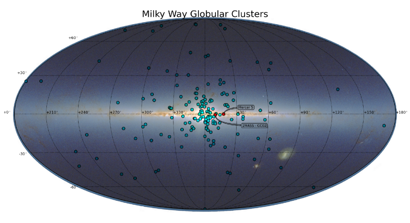
Figure 1: Illustration of the spatial distribution of the Milky Way Globular Clusters around the plane of the Galaxy. The two clusters targeted by the current study are marked and labeled. An elliptical projection of the Galactic coordinates was used with an all-sky image of the 2MASS stellar density set as a background.

2.1 Red Giant Stars Sample Selection and Observations

The stars observed in each cluster were selected on the basis of pre-existing Near-IR CMDs and low-resolution spectroscopy (SofI/NTT, R$\sim$1500 and ISAAC @ VLT, R$\sim$500). All of them were identified as high probability members of their host star clusters. The information about the individual stars observed is compiled in Table 3. We observed stars close to the Tip of the Red Giant Branch (TRGB) in order to ensure that the spectra will reach the required S/N ($\sim 60$) with a sensible investment of observing time. Figure 2 shows the positions of the target stars in the clusters, and on their color-magnitude diagrams. The J, H and Ks images are taken from the Vista variables in the Via Lactea Survey (VVV, DR2, http://horus.roe.ac.uk/vsa/, Saito et al. (2012)) and UKIDS Galactic Plane Surveys (GPS,DR7, http://www.ukidss.org/index.html) and the three-color images are constructed. The CMDs of the clusters are build using the photometric catalogs provided in VVV and GPS and include all objects residing into a 60″  radius.

The spectra were acquired at Gemini South 8-m telescope during the semester 2010A (Program GS-2010A-Q-30, PI P.Pessev). Since our targets are relatively faint for such high spectral resolution (H$\sim$10-11), our observations took full advantage of the queue mode of operation, allowing us to impose exactly the required sky and seeing conditions during the data acquisition. A standard technique of ABBA offset pattern across the slit was used. Due to the crowded nature of the observed fields (see Figure 2) we did a quick pre-imaging for the Phoenix acquisitions and provided detailed finder charts for the queue observers. Telluric standards, of spectral class A or earlier, from the Gemini calibration library were observed either before or/and after the observations at matching airmass to ensure proper reduction and calibration. Since standard stars are significantly brighter than the science targets a larger offset along the slit (4″) was used, with respect to that of the science data (2.5″). According to the standard Gemini procedure, the exposure times for the tellurics were adjusted by the night observer (depending on the luminosity of the particular star and the observing conditions at the moment of the observation) to provide sufficient S/N for high quality calibration. In general the exposure times for the standards were much shorter with respect to those of the science targets. Flat fields were taken each time science data were acquired, before moving the grating or changing the instrument configuration, using the dedicated 100W GCAL calibration source. Phoenix darks with exposure times matching the flat field data were secured at the end of each night. The calibration dataset was completed by wavelength calibration frames acquired with the internal Phoenix ThAr lamp. Considering the significant investment of observing time required and taking into account the narrow wavelength coverage of Phoenix (that does not provide a favorable configuration of calibration lines on the detector), these were taken only for a fraction of the data as an extra wavelength reference cross-check.

Slit width		4	[pix.]
Slit width		0.34	[arcsec.]
Resolution ($\lambda$/$\Delta\lambda$)		$\sim$ 50000
Central wavelength		$\sim$ 15537.5	[Å]
Wavelength coverage	min.	$\sim$ 15500.0	[Å]
	max.	$\sim$ 15575.0	[Å]
Width of the observed spectral region		75	[Å]
Filter used		H6420

Table 2: Phoenix configuration used during the observations

Table 3: Observing log and information about the individual targeted stars

Cluster ID	StarID	RA	DEC	D cen.	H	Date Obs.	Exp. Time
		hh:mm:ss	dd:mm:ss	arcsec.	mag.	DDMMYYYY	sec.
(1)	(2)	(3)	(4)	(5)	(6)	(7)	(8)
2M GC02	Star 1	18:09:35.20	-20:47:02.20	32.56	10.7	04062010UT	7200
2M GC02	Star 4	18:09:36.50	-20:46:44.10	7.50	9.7	07062010UT	7200
Mercer 5	Star 1	18:23:19.08	-13:40:09.90	8.05	9.9	02072010UT	3000
Mercer 5	Star 2	18:23:19.58	-13:40:06.70	10.04	9.1	07062010UT	2400
Notes: Columns (1) and (2) are respectively the cluster and star ID, followed by the equa-
torial coordinates of the object (columns (3) and (4)). Column (5) is showing the distance
between the individual star and the center of the corresponding cluster. The H magnitude
of the object is given in column (6). The last two columns (7) and (8) are listing the UT
date of the observation and the total exposure time used for the observations.

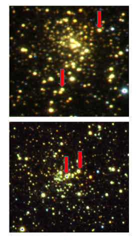
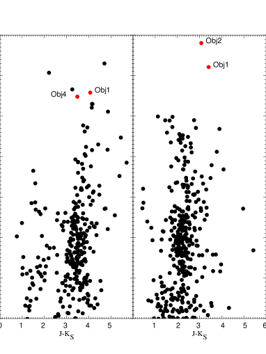
Figure 2: Illustration of the spatial distribution of the targeted red giants into the clusters and their positions on the CMDs. Left panel shows $1^{\prime}$ x $1^{\prime}$ three color images of the fields of GC02 and Mercer 5, taken from Vista variables in the Via Lactea (VVV) and UKIDS Galactic Plane Surveys. Right: The color-magnitude diagrams of the GC02 and Mercer 5 cluster fields. The black points represent all objects residing into a 60″radius; the observed objects are labeled.

2.2 Data Reduction

The reduction of the spectra was carried out in the IRAF environment, using the standard procedure for Phoenix data. Here we provide only a brief outline, with a focus on some crucial steps. First we need to trim all the science and calibration frames. This is important because a small section of the detector array is delaminated and the first $\sim$ 50 rows of each image are infested with a lot of bad pixels. Skipping that step will cause unnecessary complications during the entire data reduction process. Further the flats and darks associated with each set of observations were combined and subtracted from the combined flats. The step of developing the normalized master flat for each set is particularly important, in order to properly remove the features due to variations in the slit illumination. Normalization is also crucial for the reduction of the telluric standards, to avoid spurious features affecting the final results. OH airglow lines were removed from both standard and science targets stellar spectra by subtracting each one of the ABBA pairs. Then the two-dimensional frames were divided by the normalized flat fields before the extraction of the individual spectra. The one-dimensional spectra were wavelength calibrated, using atmospheric OH airglow lines. We targeted a spectral region that contains multiple interesting lines of Iron and $\alpha$–process elements being devoid of bright airglow features. This is particularly beneficial for the data reduction and the analysis of weak spectral lines, but poses significant challenges for the wavelength calibration. Most of the available atlases of the OH airglow are not suitable for analysis of such high-resolution data, especially taking into account the width of the analyzed spectral region (see Table 2). Fortunately the long exposures on the science targets allowed to identify five airglow features and assign the corresponding wavelengths using the The Arcturus Atlas (telluric lines) obtained with Phoenix at Kitt Peak (Hinkle et al., 1995). The wavelength calibration solution was then cross-checked against the obtained arc lamp exposures. The telluric features in the final one-dimensional spectrum were corrected using the data for the corresponding standard stars. The resulting spectra for each of the stars in both 2MASS GC02 and Mercer 5 are presented on Figure 3.

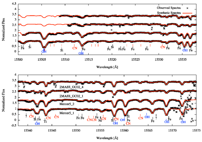
Figure 3: Observed spectra are shown with black crosses. Our best synthetic spectra are shown with a red line. Metal and Molecular lines are indicated below the spectra.

2.3 Analysis of the Obtained Spectra

Stellar spectra and chemical abundances were analyzed using the MOOG code (Sneden, 1973). To perform the analysis the program relies on stellar atmospheres models and line lists of the atomic and molecular species in the studied wavelength range. The model atmospheres were computed with the ATLAS9 Kurucz, R.L. (1993) code. Recently a significant progress was achieved on the availability of the high resolution near-IR line lists, but it is still much more limited, compared to the optical wavelength range. Pioneering works of Wallace et al. (1996) and Hinkle et al. (1995) focused on hight-resolution, high signal-to-noise spectra of the Sun and Arcturus. Current effort is aimed on provide more uniform coverage across the HR diagram (see Lebzelter et al. (2012)). Although this is a massive improvement over the earlier situation, more data and further studies are needed to match the optical spectral atlases for reference stars. The line list we used was kindly provided by Nills Ryde (private communication). It covers 699 atomic and molecular lines in the 15500 - 15575 A wavelength region (see Table 6), including Iron lines, lines of $\alpha$–elements and molecular lines (CN and OH).

MOOG computes synthetic spectra based input parameters, such as effective temperature, surface gravity, metallicity, micro-turbulence and $\alpha$-elements abundance. In order to determine the effective temperature we used the photometry and low-resolution spectroscopy published by Borissova et al. (2002) and Borissova et al. (2007) for 2MASS GC02 and Longmore et al. (2011) for Mercer 5 in conjunction with the $T_{eff}$:color:[Fe/H] calibrations of Ramírez & Meléndez (2005) for giant stars. The initial effective temperatures used were 4000K for the 2MASS GC02 stars and 3600K for Mercer 5. Surface gravity ($log\ g$) has been estimated from theoretical evolutionary tracks using the location of the stars on the red giant branch Origlia et al. (1997). We performed spectral synthesis on suitable Fe I and Fe II lines to derive the metallicity. The micro-turbulence velocity is set to a value typical for red giant stars ($\xi_{micro}$[km $s^{-1}$] = 2.13 - 0.23 log g) as given in Kirby et al. (2009). The adopted [$\alpha/Fe$]$=0.40$ is set in accordance with Gonzalez et al. (2011). Their results are based on the analysis of 650 giants in the different sections of the Galactic Bulge. To fit the widths and shapes of the lines of the observed spectra, each synthetic spectrum was convolved with a gaussian function and macro-turbulence function and the abundance is allowed to vary until the best fit is identified. The selected spectral range gives a reasonable number of atomic and molecular lines not affected by blending to derive relative abundances (see Figure 3). Unfortunately it does not cover CO molecular lines. Therefore, we adopted three values of $[C/Fe]$ = -0.15, -0.35, and -0.55 in accordance with the results of Ryde et al. (2009) and Ryde et al. (2010). The total abundance errors were determined by varying each of the input stellar parameters by its estimated errors and adding in quadrature the resulting abundance variations (see Table 4). We estimate the typical uncertainties of $\Delta T_{eff}\pm$ 100K, $\Delta$ log g $\pm$ 0.2 dex, $\Delta\xi_{micro}\pm$ 0.5 km $s^{-1}$, which translates into abundance errors for Fe$\sim$0.14, N$\sim$0.10, O$\sim$0.11, Si$\sim$0.14, Ti$\sim$0.17, Ni$\sim$0.17, respectively.

Table 4: Stellar parameters and derived abundances

		Mercer 5			2MASS GC02
Object:		#1	#2		#1	#4
$T_{eff}$ (K)		3650$\pm$100	3680$\pm$100		4000$\pm$100	4050$\pm$100
Log g $(cm\,s^{-2})$		0.5$\pm$0.2	0.5$\pm$0.2		1.0$\pm$0.2	1.0$\pm$0.2
$\xi_{micro}$ $(km\,s^{-2})$		2.0$\pm$0.5	2.0$\pm$0.5		1.9$\pm$0.5	1.9$\pm$0.5
$[\alpha/Fe]$ (dex)		0.40	0.40		0.40	0.40
$[Fe/H]$ (dex)		-0.90$\pm$0.13	-0.80$\pm$0.14		-1.10$\pm$0.14	-1.05$\pm$0.14
			$[C/Fe]$ = -0.15 dex
$[N/Fe]$ (dex)		+0.45$\pm$0.09	+0.65$\pm$0.10		+0.53$\pm$0.10	+0.43$\pm$0.10
$[O/Fe]$ (dex)		+0.30$\pm$0.11	+0.30$\pm$0.11		+0.12$\pm$0.12	+0.33$\pm$0.12
$[Si/Fe]$ (dex)		+0.50$\pm$0.14	+0.55$\pm$0.14		+0.03$\pm$0.15	0.00$\pm$0.15
$[Ti/Fe]$ (dex)		+0.30$\pm$0.17	+0.48$\pm$0.17		+0.20$\pm$0.17	+0.35$\pm$0.17
$[Ni/Fe]$ (dex)		+0.30$\pm$0.17	+0.25$\pm$0.17		+0.20$\pm$0.17	+0.10$\pm$0.17
			$[C/Fe]$ = -0.35 dex
$[N/Fe]$ (dex)		+0.65$\pm$0.10	+0.95$\pm$0.10		+0.75$\pm$0.10	+0.70$\pm$0.10
$[O/Fe]$ (dex)		+0.30$\pm$0.10	+0.32$\pm$0.11		+0.10$\pm$0.12	+0.35$\pm$0.12
$[Si/Fe]$ (dex)		+0.50$\pm$0.14	+0.55$\pm$0.14		+0.05$\pm$0.15	+0.02$\pm$0.15
$[Ti/Fe]$ (dex)		+0.40$\pm$0.17	+0.48$\pm$0.17		+0.30$\pm$0.17	+0.35$\pm$0.17
$[Ni/Fe]$ (dex)		+0.30$\pm$0.17	+0.25$\pm$0.17		+0.15$\pm$0.17	+0.10$\pm$0.17
			$[C/Fe]$ = -0.55 dex
$[N/Fe]$ (dex)		+0.90$\pm$0.10	+1.15$\pm$0.11		+1.03$\pm$0.10	+0.90$\pm$0.10
$[O/Fe]$ (dex)		+0.30$\pm$0.10	+0.32$\pm$0.11		+0.15$\pm$0.11	+0.30$\pm$0.11
$[Si/Fe]$ (dex)		+0.50$\pm$0.14	+0.55$\pm$0.14		+0.03$\pm$0.15	0.00$\pm$0.15
$[Ti/Fe]$ (dex)		+0.40$\pm$0.17	+0.48$\pm$0.17		+0.20$\pm$0.17	+0.40$\pm$0.17
$[Ni/Fe]$ (dex)		+0.30$\pm$0.17	+0.25$\pm$0.17		+0.15$\pm$0.17	+0.10 $\pm$0.17

3 Results

Figure 3 shows our best-fitting synthetic spectra superimposed on the observed spectra of the target giants in both globular clusters. The derived stellar parameters and element abundances are summarized in Table 4. By definition:

$$[X/Fe]=({log\epsilon(X)-log\epsilon(Fe)}_{star})-({log\epsilon(X)-log\epsilon(Fe)}_{\odot})$$ (1)

$$log\epsilon(X)=log\,n_{X}/n_{H}+12,$$ (2)

where $log\,n_{X}$ is the number density of element X.

As mentioned before, the observed spectral interval does not cover the CO molecular lines, hence we can not derive C abundance. To approach this we estimate the [N/Fe], [O/Fe], [Si/Fe], [Ti/Fe], [Ni/Fe] abundances for three distinct [C/Fe] values, consistent with the range reported for 14 red giants in the Galactic bulge by Ryde et al. (2009) and Ryde et al. (2010). As evident from the table, taking into account the uncertainties, most of the estimates for the individual giants are in agreement and only the [N/Fe] is affected by variations of [C/Fe]. In Table 5 we present the mean [O/Fe], [Si/Fe], [Ti/Fe], [Ni/Fe] abundances for each observed giant in Mercer 5 and 2MASS GC02 based on three estimates per star ([Fe/H] values for each star are also listed ). For each cluster, [Fe/H] is calculated as the mean for the two giants, [O/Fe], [Si/Fe], [Ti/Fe], [Ni/Fe] are the mean of all the individual estimates. The uncertainties of the individual measurements were used to calculate the corresponding weights. The uncertainties reported in the table represent a conservative estimate, taking into account observational uncertainties, errors of calibrations, transformations and determination of the atmospheric parameters.

To compare our determinations with the abundance rations measured by previous authors we selected four bulge globular clusters: NGC 6522 (Barbuy et al. (2014)); NGC 6569 and NGC 6624 (Valenti et al. (2011)) and Terzan 1 (Valenti et al. (2014)); as well as the abundance measurements of 264 red giant stars in three bulge fields taken from Johnson et al. (2013). The results are shown in Figure 4 and Figure 5.

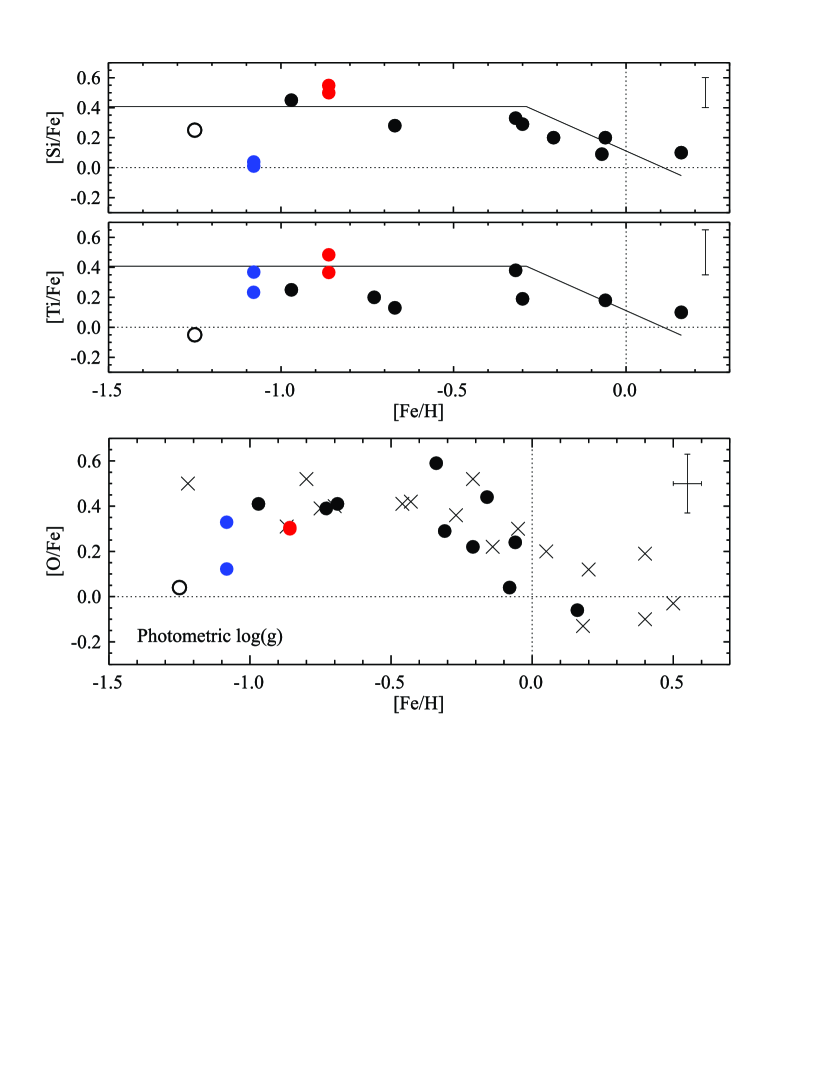
Figure 4: The ratios of O, Si and Ti to Iron (top to bottom). The dark circles stand for NGC 6522 red giant stars; blue, green and pink circles are for NGC 6569, NGC 6624 and Terzan 1 red giants, the Mercer 5 and 2MASS GC02 red giant abundance ratios from this paper are presented as red circles and are labeled.

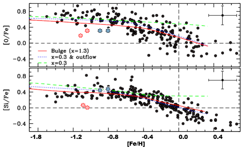
Figure 5: On the Fig. 18 of Johnson et al. (2013) are overplotted [O/Fe] and [Si/Fe] abundance rations of Mercer 5 (blue stars) and 2MASS GC02 (red stars) objects. The black circles are abundance rations of 264 red giants of three combined bulge fields; the solid red line shows the predicted change in each $\alpha$-element as a function of [Fe/H], based on the bulge model of Kobayashi et al. (2011). The dashed green line is the model prediction assuming a flatter IMF (x=0.3) and the dotted blue line is the model prediction assuming x=0.3 with outflow (see Johnson et al. (2013) for details).

As can be seen from the plots, the two measured stars of Mercer 5 follow the general trend of both bulge field and cluster stars at this metallicity. Indeed, their [O/Fe], [Si/Fe] and [Ti/Fe] ratios are enhanced by $\geq+$ 0.3. The 2MASS GC02 stars have relatively lower ratios, but still compatible with other bulge clusters. Therefore, abundance ratios alone would not allow us to confirm that these two objects are indeed bound globular clusters. On the other hand, the bulge metallicity distribution is populated only very sparsely at [Fe/H]$\sim$-1.0, therefore if those 4 were just bulge field stars, the probability of having all of them so metal poor is virtually zero. Hence we confirm the cluster nature of both Mercer 5 and 2MASS GC02.

	Mercer 5			2MASS GC02
	Object #1	Object #2	Mean	Object #1	Object #4	Mean
[Fe/H]	$-0.90\pm 0.13$	$-0.80\pm 0.14$	$-0.86\pm 0.14$	$-1.10\pm 0.14$	$-1.05\pm 0.14$	$-1.08\pm 0.13$
[O/Fe]	$0.30\pm 0.11$	$0.31\pm 0.11$	$0.31\pm 0.11$	$0.15\pm 0.12$	$0.33\pm 0.12$	$0.23\pm 0.12$
[Si/Fe]	$0.50\pm 0.14$	$0.55\pm 0.14$	$0.53\pm 0.14$	$0.04\pm 0.15$	$0.00\pm 0.15$	$0.02\pm 0.15$
[Ti/Fe]	$0.37\pm 0.17$	$0.48\pm 0.17$	$0.42\pm 0.17$	$0.23\pm 0.17$	$0.37\pm 0.17$	$0.30\pm 0.17$
[Ni/Fe]	$0.30\pm 0.17$	$0.25\pm 0.17$	$0.28\pm 0.17$	$0.17\pm 0.17$	$0.10\pm 0.17$	$0.13\pm 0.17$

Table 5: Derived abundances for both clusters. The mean [O/Fe], [Si/Fe], [Ti/Fe], [Ni/Fe] abundances for each observed giant in Mercer 5 and 2MASS GC02 are based on three estimates per star, ([Fe/H] values for each star are also listed ). For each cluster, [Fe/H] is calculated as the mean for the two giants, [O/Fe], [Si/Fe], [Ti/Fe], [Ni/Fe] are the mean of the six individual estimates.

4 Summary

We present the first chemical abundance estimates of two newly discovered Galactic globular clusters, residing in the direction of the Bulge in regions of high interstellar reddening. [Fe/H] for 2MASS GC02 is in agreement with earlier estimate by Borissova et al. (2007) based on moderate-resolution near-IR spectroscopy in the K band. The metallicity for Mercer 5 is significantly higher than the value derived by Longmore et al. (2011) using SofI/NTT moderate-resolution spectra. Based on these results we conclude that both Mercer 5 and 2MASS GS02 are two intermediate metal reach Bulge globular clusters, with Iron abundances of [Fe/H]=$-0.86$ and [Fe/H]=$-1.08$, respectively. The [O/Fe], [Si/Fe] and [Ti/Fe] abundance rations of Mercer 5 are enhanced by $\geq+$ 0.3, with respect to solar value, while the two observed giants of 2MASS GC02 show lower rations.

, No. Wav.[$\AA$] Elem. $\chi_{\mathrm{exc}}$[eV] No. Wav. [$\AA$] Elem. $\chi_{\mathrm{exc}}$[eV] No. Wav.[$\AA$] Elem. $\chi_{\mathrm{exc}}$[eV] No. Wav.[$\AA$] Elem. $\chi_{\mathrm{exc}}$[eV] 1 15500.073 ScI 4.50 176 15520.653 CN 3.76 351 15538.772 CN 3.75 526 15557.847 CN 2.65 2 15500.241 VII 9.04 177 15520.684 CN 3.36 352 15538.799 CN 4.15 527 15558.023 OH 0.30 3 15500.316 TiI 4.36 178 15520.855 CN 2.94 353 15538.854 CN 2.89 528 15558.045 CN 0.91 4 15500.345 CN 0.86 179 15520.893 OH 2.19 354 15538.903 CN 2.53 529 15558.176 CN 2.66 5 15500.650 MnI 6.20 180 15521.086 FeI 5.35 355 15539.060 CN 4.13 530 15558.585 TiI 4.50 6 15500.708 CN 2.58 181 15521.135 CN 4.00 356 15539.126 OH 0.79 531 15558.665 CN 0.73 7 15500.800 FeI 6.32 182 15521.207 CN 5.20 357 15539.330 CN 4.25 532 15558.880 CN 2.64 8 15501.003 CN 0.86 183 15521.245 CN 1.72 358 15539.417 CrI 5.96 533 15558.960 CN 2.87 9 15501.080 CN 3.15 184 15521.383 CN 2.40 359 15539.666 CN 2.53 534 15559.103 CN 2.42 10 15501.080 FeI 5.94 185 15521.515 CN 4.41 360 15539.673 CN 4.42 535 15559.500 NiI 5.87 11 15501.320 FeI 6.29 186 15521.690 FeI 6.32 361 15539.758 CN 3.29 536 15559.542 CN 1.01 12 15501.345 CN 3.29 187 15522.054 OH 2.83 362 15539.777 CN 5.82 537 15559.556 CN 2.67 13 15501.354 OH 3.10 188 15522.230 OH 3.12 363 15539.837 CN 0.88 538 15559.566 CN 1.00 14 15501.511 CN 0.99 189 15522.236 OH 2.73 364 15539.992 CN 5.16 539 15559.648 CN 1.01 15 15501.787 CN 2.84 190 15522.287 CN 2.94 365 15540.312 OH 3.48 540 15559.660 CN 1.00 16 15501.833 CN 2.58 191 15522.460 CN 4.21 366 15540.463 CN 3.98 541 15559.801 CN 1.00 17 15502.170 FeI 6.35 192 15522.600 CoI 6.21 367 15540.516 CN 0.88 542 15559.849 FeI 5.93 18 15502.239 CN 5.50 193 15522.640 FeI 6.32 368 15540.518 CN 3.77 543 15559.922 CaI 5.17 19 15502.261 CN 0.99 194 15522.672 OH 2.19 369 15540.898 CN 4.96 544 15559.973 CN 0.99 20 15502.294 OH 2.94 195 15523.041 CN 5.20 370 15541.125 CN 4.04 545 15560.135 CN 2.51 21 15502.429 CoI 3.41 196 15523.051 OH 2.73 371 15541.299 CN 3.98 546 15560.149 CN 1.01 22 15502.434 CN 3.98 197 15523.386 CN 3.72 372 15541.516 CN 5.73 547 15560.208 CN 1.00 23 15502.549 CN 2.84 198 15523.511 CN 1.45 373 15541.547 FeI 5.84 548 15560.244 OH 0.30 24 15502.564 CN 2.55 199 15523.591 OH 3.19 374 15541.557 CN 3.83 549 15560.270 CN 1.01 25 15502.576 CN 2.56 200 15523.807 CN 4.21 375 15541.644 OH 0.89 550 15560.287 CN 1.00 26 15502.640 SiI 7.13 201 15523.909 CN 0.88 376 15541.654 CN 4.42 551 15560.324 CN 3.71 27 15502.836 OH 3.44 202 15523.998 CoI 6.05 377 15541.818 CN 3.58 552 15560.578 CN 1.00 28 15502.934 CN 2.56 203 15524.003 CN 3.46 378 15541.850 CN 1.26 553 15560.685 CN 2.51 29 15503.043 OH 2.86 204 15524.277 NiI 2.74 379 15541.852 FeI 5.97 554 15560.704 CN 2.64 30 15503.246 ScI 4.17 205 15524.300 FeI 5.79 380 15541.857 FeI 6.37 555 15560.780 FeI 6.35 31 15503.246 CrI 3.38 206 15524.451 CN 0.88 381 15542.016 SiI 7.01 556 15561.041 CoI 6.08 32 15503.441 OH 2.72 207 15524.543 FeI 5.79 382 15542.090 SiI 7.01 557 15561.242 CN 3.72 33 15503.840 FeI 5.97 208 15524.615 CN 4.21 383 15542.090 FeI 5.64 558 15561.251 SiI 7.04 34 15503.943 CoI 5.73 209 15524.822 CN 2.55 384 15542.108 CN 0.83 559 15561.268 FeI 6.71 35 15503.967 VI 4.72 210 15524.832 CN 4.55 385 15542.146 OH 0.89 560 15561.399 CN 1.01 36 15503.994 CN 3.37 211 15524.847 OH 0.84 386 15542.173 CN 4.13 561 15561.457 CN 1.00 37 15504.083 CN 3.21 212 15525.227 FeI 5.84 387 15542.197 TiI 4.69 562 15561.523 CN 1.00 38 15504.126 CN 3.72 213 15525.360 CN 5.82 388 15542.205 CN 5.20 563 15561.535 CN 1.01 39 15504.554 CN 3.72 214 15525.406 CN 4.61 389 15542.297 CN 1.91 564 15561.748 CN 2.68 40 15505.107 CN 3.94 215 15525.435 CN 4.67 390 15542.316 CN 5.12 565 15562.080 VI 4.63 41 15505.326 OH 0.52 216 15525.495 CN 4.41 391 15542.611 CN 5.08 566 15562.131 CN 4.25 42 15505.350 CN 5.21 217 15525.514 CN 2.94 392 15542.731 TiI 4.39 567 15562.143 CN 2.50 43 15505.524 OH 1.43 218 15525.531 CN 2.72 393 15542.980 CN 1.20 568 15562.291 CN 1.15 44 15505.526 CN 1.45 219 15525.661 VI 4.88 394 15543.326 CN 4.00 569 15562.300 NiI 6.37 45 15505.591 CN 2.99 220 15525.734 TiII 8.10 395 15543.357 TiI 4.86 570 15562.436 CN 6.54 46 15505.747 OH 0.52 221 15525.738 TiI 4.79 396 15543.633 CN 4.05 571 15562.441 CN 2.50 47 15505.771 TiI 4.39 222 15525.775 OH 3.51 397 15543.780 TiI 1.88 572 15562.460 CN 6.32 48 15505.782 OH 1.89 223 15525.775 CN 2.55 398 15543.785 OH 0.84 573 15562.601 OH 2.77 49 15505.846 CN 4.27 224 15525.934 CN 2.51 399 15543.838 TiI 4.79 574 15563.095 OH 2.77 50 15505.849 OH 1.43 225 15525.963 CN 4.21 400 15543.846 CN 3.58 575 15563.136 CN 3.58 51 15506.052 OH 2.85 226 15526.062 CN 2.84 401 15544.152 CuI 6.79 576 15563.139 OH 2.75 52 15506.079 CN 2.44 227 15526.083 CN 5.15 402 15544.355 TiI 2.49 577 15563.165 CN 4.29 53 15506.099 OH 1.43 228 15526.404 CN 1.00 403 15544.452 CN 2.72 578 15563.303 CN 1.00 54 15506.105 FeI 5.52 229 15526.414 CN 3.77 404 15544.501 CN 1.15 579 15563.306 CN 1.02 55 15506.246 OH 1.43 230 15526.604 CN 2.45 405 15544.680 CN 2.79 580 15563.315 CN 2.63 56 15506.246 OH 1.89 231 15526.819 CN 5.39 406 15544.730 CN 2.86 581 15563.354 CN 1.00 57 15506.252 ScI 4.97 232 15526.841 CN 3.84 407 15544.771 CN 4.00 582 15563.376 CN 1.15 58 15506.363 CN 4.26 233 15526.865 CN 4.55 408 15544.899 CN 4.47 583 15563.456 CN 1.02 59 15506.408 CN 4.91 234 15526.976 CN 2.72 409 15544.948 CN 2.51 584 15563.463 CrI 5.24 60 15506.685 CN 2.71 235 15527.043 CN 3.15 410 15545.047 CN 4.41 585 15563.778 CN 2.46 61 15506.779 CN 1.45 236 15527.210 FeI 6.32 411 15545.332 CN 2.72 586 15563.902 CN 2.79 62 15506.901 CN 6.39 237 15527.323 CN 3.90 412 15545.409 CN 5.63 587 15564.020 FeII 9.05 63 15506.969 CN 5.52 238 15527.325 CN 3.84 413 15545.511 CN 2.86 588 15564.185 CN 4.25 64 15506.980 SiI 6.73 239 15527.465 CN 2.57 414 15545.584 CN 1.15 589 15564.268 CN 2.75 65 15507.022 VI 4.87 240 15527.470 CN 2.94 415 15545.668 CN 5.82 590 15564.369 FeI 5.61 66 15507.043 PI 8.23 241 15527.513 CN 3.94 416 15545.782 CN 1.22 591 15564.684 CN 2.73 67 15507.046 CN 1.00 242 15527.535 SiI 7.14 417 15546.081 TiI 4.41 592 15564.723 ScI 4.53 68 15507.046 CN 3.21 243 15527.564 CN 4.61 418 15546.089 CN 2.60 593 15564.769 CN 2.69 69 15507.048 CN 2.99 244 15527.629 CN 4.55 419 15546.488 CN 2.60 594 15564.793 CN 2.75 70 15507.103 TiI 4.77 245 15527.713 OH 2.89 420 15546.531 CN 4.47 595 15564.938 OH 0.78 71 15507.118 FeII 8.94 246 15527.837 CN 2.57 421 15546.709 OH 3.48 596 15565.230 FeI 6.32 72 15507.156 CN 0.89 247 15527.890 CN 4.42 422 15546.780 CN 2.83 597 15565.256 CN 2.58 73 15507.180 CN 2.71 248 15528.109 FeI 5.95 423 15546.790 CN 4.47 598 15565.336 CN 2.42 74 15507.241 CN 0.71 249 15528.121 OH 1.35 424 15546.818 OH 2.75 599 15565.356 CN 0.91 75 15507.332 CN 5.21 250 15528.128 CN 4.92 425 15546.838 CN 1.22 600 15565.390 CN 4.05 76 15507.500 CN 4.49 251 15528.160 CN 2.96 426 15546.848 CN 5.44 601 15565.448 CN 1.76 77 15507.623 TiI 5.24 252 15528.218 CN 1.00 427 15546.920 CN 1.55 602 15565.588 CN 5.35 78 15507.816 CN 2.38 253 15528.365 CN 4.88 428 15547.041 CN 4.21 603 15565.644 CN 2.79 79 15507.844 CN 0.89 254 15528.575 CN 2.72 429 15547.940 OH 1.56 604 15565.734 CN 0.99 80 15508.075 CN 2.64 255 15528.577 CN 4.35 430 15548.190 CN 0.99 605 15565.770 CN 0.99 81 15508.385 TiI 4.77 256 15528.589 CN 2.67 431 15548.349 CN 3.67 606 15565.817 OH 0.90 82 15508.393 CN 4.80 257 15528.599 CN 4.67 432 15548.422 CN 4.47 607 15565.838 OH 3.66 83 15508.477 CN 1.22 258 15528.618 CN 3.77 433 15548.480 CN 3.89 608 15565.879 CN 1.02 84 15508.670 OH 1.89 259 15528.631 OH 3.06 434 15548.487 OH 3.66 609 15565.886 VI 4.64 85 15508.677 CN 6.07 260 15528.670 OH 3.21 435 15548.673 CN 2.87 610 15565.962 OH 2.78 86 15508.718 CN 2.64 261 15528.768 CN 3.94 436 15548.908 CN 2.61 611 15565.996 OH 0.90 87 15508.799 CN 0.97 262 15528.891 CN 4.41 437 15548.914 OH 0.93 612 15566.044 CN 1.02 88 15509.016 CN 3.46 263 15528.903 CN 2.94 438 15548.978 CaI 5.18 613 15566.051 CN 5.16 89 15509.507 CN 2.48 264 15528.915 CN 3.15 439 15549.206 CN 3.19 614 15566.255 CN 4.12 90 15509.526 CN 0.97 265 15528.994 CN 1.00 440 15549.501 CN 3.90 615 15566.274 CN 6.40 91 15509.779 CN 2.48 266 15528.994 CN 3.06 441 15549.541 OH 2.59 616 15566.393 CN 4.96 92 15509.863 CN 2.70 267 15529.105 CN 4.92 442 15549.554 CN 2.83 617 15566.603 OH 2.68 93 15510.178 CN 4.20 268 15529.168 CN 2.96 443 15549.736 OH 2.18 618 15566.703 CN 2.63 94 15510.358 OH 1.89 269 15529.226 CN 5.84 444 15549.786 CN 3.90 619 15566.725 FeI 6.35 95 15510.648 OH 0.26 270 15529.243 CN 2.77 445 15549.803 CN 4.03 620 15566.907 CN 4.50 96 15510.717 CN 3.46 271 15529.316 OH 3.06 446 15549.902 OH 0.73 621 15566.941 CN 3.84 97 15510.847 CN 2.72 272 15529.344 CN 4.61 447 15549.948 CN 2.87 622 15567.001 ScI 4.97 98 15511.088 CN 4.20 273 15529.453 CN 2.72 448 15550.226 CN 4.10 623 15567.014 CN 3.94 99 15511.117 SiI 7.17 274 15529.657 OH 3.48 449 15550.320 CN 2.66 624 15567.188 SiI 7.11 100 15511.528 FeI 5.48 275 15529.662 CN 4.55 450 15550.357 CN 4.03 625 15567.261 FeI 6.35 101 15511.665 CN 5.73 276 15529.773 CN 3.15 451 15550.381 CN 0.89 626 15567.530 CN 6.42 102 15511.769 CN 5.52 277 15529.846 CN 4.67 452 15550.450 FeI 6.34 627 15567.552 OH 3.00 103 15511.810 CN 0.88 278 15529.913 CN 1.25 453 15550.553 CN 2.65 628 15567.575 OH 0.73 104 15512.147 CN 3.62 279 15529.928 CN 2.67 454 15550.560 FeI 6.11 629 15567.680 VI 4.62 105 15512.291 CN 2.37 280 15530.010 CN 2.64 455 15550.623 CN 3.19 630 15567.704 CN 5.16 106 15512.575 OH 0.86 281 15530.043 FeI 3.57 456 15550.645 CN 2.96 631 15567.724 CN 3.84 107 15512.635 CN 4.60 282 15530.080 CN 0.89 457 15550.867 CN 3.90 632 15567.728 VI 4.59 108 15512.724 VI 4.68 283 15530.162 CN 2.65 458 15550.949 CN 0.89 633 15567.869 CN 2.55 109 15512.761 CN 2.48 284 15530.186 CN 2.51 459 15550.964 CN 3.06 634 15568.180 CN 1.29 110 15512.771 OH 0.86 285 15530.195 VI 5.45 460 15550.981 CN 2.66 635 15568.187 SiI 7.11 111 15512.891 CN 0.82 286 15530.205 CN 3.06 461 15551.172 CN 5.44 636 15568.325 FeI 5.88 112 15513.146 CN 5.31 287 15530.316 CN 2.77 462 15551.430 FeI 6.35 637 15568.383 VI 4.67 113 15513.208 CN 1.12 288 15530.654 CN 2.64 463 15551.636 CN 2.89 638 15568.567 CN 4.96 114 15513.336 CN 2.67 289 15530.683 CN 4.30 464 15551.714 CN 4.14 639 15568.614 CN 2.69 115 15513.367 CN 3.54 290 15530.810 CN 0.89 465 15551.818 VI 4.66 640 15568.650 CN 2.45 116 15513.468 OH 0.92 291 15531.103 OH 3.29 466 15551.861 CN 2.65 641 15568.744 CN 0.99 117 15513.477 OH 0.26 292 15531.124 OH 2.94 467 15552.108 TiII 8.11 642 15568.764 CN 0.99 118 15513.511 TiI 4.51 293 15531.280 TiI 4.65 468 15552.222 FeI 5.62 643 15568.780 OH 0.30 119 15513.675 CN 1.06 294 15531.494 CN 4.84 469 15552.254 OH 2.74 644 15568.853 OH 3.29 120 15513.800 OH 0.92 295 15531.503 CN 4.61 470 15552.268 CN 3.89 645 15568.955 CN 2.86 121 15514.195 CN 2.53 296 15531.646 CN 3.15 471 15552.747 CN 0.90 646 15568.980 CN 4.50 122 15514.270 CN 1.12 297 15531.713 CN 3.12 472 15552.769 CN 3.89 647 15569.103 SiI 7.11 123 15514.280 FeI 6.29 298 15531.750 FeI 5.64 473 15552.885 CN 4.14 648 15569.135 CN 1.03 124 15514.427 OH 3.12 299 15532.116 CN 4.35 474 15553.245 VII 5.54 649 15569.240 FeI 5.51 125 15514.496 CN 1.06 300 15532.263 SiI 7.14 475 15553.313 CN 4.14 650 15569.314 CN 1.03 126 15514.691 SiI 7.09 301 15532.449 SiI 6.72 476 15553.340 CN 2.58 651 15569.486 CN 4.21 127 15514.802 CN 1.33 302 15532.536 CN 4.29 477 15553.560 FeI 5.48 652 15569.490 OH 0.84 128 15514.891 CN 1.52 303 15532.802 OH 3.48 478 15553.577 CN 2.89 653 15569.576 CN 4.74 129 15515.117 OH 2.21 304 15533.347 CN 4.29 479 15553.659 CN 1.08 654 15569.741 CoI 5.75 130 15515.368 TiI 2.31 305 15533.389 OH 1.35 480 15553.727 CN 2.58 655 15569.903 CN 2.61 131 15515.373 VI 4.65 306 15533.710 OH 2.33 481 15554.146 CN 4.41 656 15569.911 CN 2.40 132 15515.416 CN 2.38 307 15533.849 CN 0.99 482 15554.446 OH 0.79 657 15569.984 OH 2.78 133 15515.445 OH 2.18 308 15533.977 SiI 7.14 483 15554.501 CN 1.08 658 15570.044 CN 3.81 134 15515.617 OH 2.18 309 15534.020 CN 3.67 484 15554.510 FeI 6.28 659 15570.073 CN 3.70 135 15515.768 FeI 6.29 310 15534.081 CN 4.29 484 15554.510 fEi 6.28 660 15570.202 NiII 8.42 136 15515.777 CN 2.50 311 15534.182 CN 3.36 486 15554.557 TiI 4.43 661 15570.306 CN 3.10 137 15515.797 CN 1.33 312 15534.260 FeI 5.64 487 15554.603 CN 1.28 662 15570.575 CN 3.41 138 15515.876 TiI 4.79 313 15534.306 OH 0.84 488 15554.625 VI 4.61 663 15570.752 CN 5.08 139 15515.931 CN 1.18 314 15534.368 CN 3.68 489 15554.697 VII 5.87 664 15570.861 CN 2.62 140 15515.969 OH 3.06 315 15534.399 CN 2.45 490 15554.855 CN 5.01 665 15571.055 CN 2.61 141 15516.151 CN 4.82 316 15534.455 CN 2.83 491 15554.939 OH 2.75 666 15571.099 VI 4.68 142 15516.284 OH 2.83 317 15534.602 CN 0.99 492 15555.112 OH 3.66 667 15571.120 FeI 5.88 143 15516.418 CN 1.00 318 15534.665 CN 4.13 493 15555.120 NiI 5.28 668 15571.152 CN 1.22 144 15516.537 OH 3.29 319 15534.892 CN 4.29 494 15555.138 CN 4.50 669 15571.220 CN 3.19 145 15516.660 OH 2.89 320 15534.986 CN 2.73 495 15555.210 NiI 5.28 670 15571.417 CN 4.21 146 15516.720 FeI 6.29 321 15535.167 CN 1.33 496 15555.370 NiI 5.49 671 15571.511 CN 5.35 147 15517.095 CN 2.77 322 15535.182 CN 4.27 497 15555.641 ScI 5.06 672 15571.664 CN 5.41 148 15517.228 OH 2.85 323 15535.317 CN 2.49 498 15555.700 CN 1.02 673 15571.729 VI 2.58 149 15517.275 CoI 5.74 324 15535.329 CN 3.91 499 15555.720 CN 1.36 674 15571.740 FeI 6.32 150 15517.367 CN 1.20 325 15535.353 CN 5.50 500 15555.750 CN 1.49 675 15571.822 CN 2.66 151 15517.487 CN 3.29 326 15535.462 OH 0.51 501 15555.765 OH 1.50 676 15571.834 CN 3.82 152 15517.815 CN 4.35 327 15535.498 CN 2.73 502 15555.835 CN 4.14 677 15571.897 CN 3.10 153 15518.135 CN 2.49 328 15535.602 CN 2.49 503 15556.016 NiI 5.28 678 15572.084 OH 0.30 154 15518.166 CN 2.77 329 15535.816 CN 1.06 504 15556.058 CN 4.04 679 15572.166 ScI 5.54 155 15518.289 CN 2.58 330 15535.829 CN 0.90 505 15556.106 OH 1.50 680 15572.217 CN 5.08 156 15518.395 CN 1.20 331 15536.224 CN 4.92 506 15556.115 OH 1.49 681 15572.230 OH 3.19 157 15518.670 CN 2.49 332 15536.642 CN 1.06 507 15556.122 CuI 6.55 682 15572.312 CN 0.84 158 15518.675 CN 2.58 333 15536.706 OH 0.51 508 15556.384 CN 4.30 683 15572.334 CN 0.99 159 15518.708 CN 4.14 334 15536.773 CN 2.71 509 15556.593 CN 1.02 684 15572.484 CN 2.66 160 15518.720 ScI 5.10 335 15536.895 OH 3.44 510 15556.670 FeI 5.93 685 15572.632 TiI 4.67 161 15518.764 CN 4.04 336 15536.997 CN 0.99 511 15556.711 TiI 5.30 686 15572.651 VI 4.65 162 15518.793 CN 1.23 337 15537.181 OH 0.84 512 15556.919 CN 4.04 687 15573.083 CN 1.03 163 15518.829 CN 5.07 338 15537.207 OH 0.78 513 15556.939 CN 1.36 688 15573.261 CN 1.49 164 15518.900 FeI 6.28 339 15537.227 CN 3.67 514 15556.962 OH 1.50 689 15573.277 CN 1.03 165 15519.065 CN 3.29 340 15537.253 CN 3.27 515 15557.006 CN 3.74 690 15573.294 CN 2.70 166 15519.084 CN 3.36 341 15537.410 OH 0.48 516 15557.006 CN 4.14 691 15573.466 CN 3.90 167 15519.100 FeI 6.29 342 15537.450 FeI 5.79 517 15557.212 OH 1.57 692 15573.673 CN 2.53 168 15519.360 FeI 6.29 343 15537.572 FeI 5.79 518 15557.387 CN 1.49 693 15573.724 CN 5.50 169 15519.600 CN 3.61 344 15537.690 FeI 6.32 519 15557.447 CN 3.74 694 15573.821 CN 4.68 170 15519.636 VI 4.11 345 15537.777 CN 4.13 520 15557.602 VI 4.68 695 15573.976 CrI 5.94 171 15519.942 FeI 2.48 346 15538.060 CoI 5.74 521 15557.607 CN 2.66 696 15574.060 FeI 6.31 172 15519.949 ScI 3.81 347 15538.081 CN 0.76 522 15557.684 CN 2.87 697 15574.599 CN 2.42 173 15520.115 SiI 7.11 348 15538.084 CN 5.20 523 15557.689 TiI 5.28 698 15574.667 CN 5.85 174 15520.154 CN 5.37 349 15538.434 OH 0.48 524 15557.735 CN 2.96 699 15574.837 CN 2.61 175 15520.262 CN 4.41 350 15538.463 SiI 6.76 525 15557.790 SiI 5.96

Table 6: Line list used to model the observed spectra. The wavelength is in air, the excitation energy is of the lower level.

References

- Abazajian et al. (2009) Abazajian, K. N., Adelman-McCarthy, J. K., Agüeros, M. A., et al. 2009, ApJS, 182, 543
- Alonso-García et al. (2014) Alonso-García Dé́ká́ny, I., Catelan, M., Contreras, R. Gran, F. at al. 2014, 2014arXiv1411.1696A
- Barbuy et al. (2014) Barbuy, B., Chiappini, C., Cantelli, E., Depagne, E., Pignatari, M. et al. 2014 A&A, 570, 76
- Benjamin et al. (2003) Benjamin, R. A., Churchwell, E., Babler, B. L., et al. 2003, PASP, 115, 953
- Bica et al. (2007) Bica, E., Bonatto, C., Ortolani, S., & Barbuy, B. 2007, A&A, 472, 483
- Bonatto et al. (2007) Bonatto, C., Bica, E., Ortolani, S., & Barbuy, B. 2007, MNRAS, 381, L45
- Bonatto et al. (2010) Bonatto, C. & Bica, E. 2010, A&A, 516, 81
- Borissova et al. (2002) Borissova, J., Ivanov, V. D., & Vanzi, L. 2002, Extragalactic Star Clusters, 207, 107
- Borissova et al. (2007) Borissova, J., Ivanov, V. D., Stephens, A. W., et al. 2007, A&A, 474, 121
- Ferraro et al. (2006) Ferraro, F., Valenti, E., and Origlia, L. 2006, AJ, 649, 243
- Froebrich et al. (2008a) Froebrich, D., Meusinger, H., & Davis, C. J. 2008, MNRAS, 383, L45
- Gonzalez et al. (2011) Gonzalez, O. A., Rejkuba, M., Zoccali, M., et al. 2011, A&A, 530, A54
- Gonzalez et al. (2013) Gonzalez, O. A., Rejkuba, M., Zoccali, M., et al. 2013, A&A, 552, A110
- Harris (1996) Harris, W. E. 1996, AJ, 112, 1487
- Hinkle et al. (1995) Hinkle, K., Wallace, L., & Livingston, W. 1995, PASP, 107, 1042
- Hinkle et al. (1998) Hinkle, K. H., Cuberly, R. W., Gaughan, N. A., et al. 1998, Proc. SPIE, 3354, 810
- Hurt et al. (2000) Hurt, R. L., Jarrett, T. H., Kirkpatrick, J. D., et al. 2000, AJ, 120, 1876
- Johnson et al. (2013) Johnson, C. I., Rich, R. M., Kobayashi, C., Kunder, A., & Koch, A. et al. 2013 ApJ, 765, 157
- Kobayashi et al. (2011) Kobayashi, C., Karakas, A. I., & Umeda, H. 2011, MNRAS, 414, 3231
- Kirby et al. (2009) Kirby, Evan N.; Guhathakurta, Puragra; Bolte, Michael; Sneden, Christopher; Geha, Marla C. 2009, ApJ, 705, 328
- Kurucz, R.L. (1993) Kurucz, R.L. 1993, CD ROM, no 13
- Lebzelter et al. (2012) Lebzelter, T., Seifahrt, A., Uttenthaler, S., et al. 2012, A&A, 539, A109
- Longmore et al. (2011) Longmore, A. J., Kurtev, R., Lucas, P. W., et al. 2011, MNRAS, 416, 465
- Marigo et al (2008) Marigo P., Girardi L., Bressan A., Groenewegen M. A. T., Silva L., Granato G. L.2008, A&A, 482, 883
- Martini et al. (2004) Martini, P., Persson, S. E., Murphy, D. C., et al. 2004, Proc. SPIE, 5492, 1653
- Mercer et al. (2005) Mercer, E. P., Clemens, D. P., Meade, M. R., et al. 2005, ApJ, 635, 560
- Minniti et al. (2010) Minniti, D., Lucas, P. W., Emerson, J. P., et al. 2010, New A, 15, 433
- Minniti et al. (2011) Minniti, D., Hempel, M., Toledo, I., et al. 2011, A&A, 527, A81
- Moni Bidin et al. (2011) Moni Bidin, C., Mauro, F., Geisler, D., et al. 2011, A&A, 535, A33
- Nataf et al. (2014) Nataf, D. M., Cassisi, S., & Athanassoula, E. 2014, MNRAS, 442, 2075
- Origlia et al. (1997) Origlia, L., Ferraro, F. R., Fusi Pecci, F., Oliva, E. 1997, A&A, 321, 859
- Ortolani et al. (2009) Ortolani, S., Bonatto, C., Bica, E., & Barbuy, B. 2009, AJ, 138, 889
- Ortolani et al. (2012) Ortolani, S., Bonatto, C., Bica, E., Barbuy, B., & Saito, R. K. 2012, AJ, 144, 147
- Pietrinferni et al. (2004) Pietrinferni, A., Cassisi, S., Salaris, M., & Castelli, F. 2004, AJ, 612, 168
- Ramírez & Meléndez (2005) Ramírez, I. & Meléndez, J. 2005, ApJ, 626, 465
- Roediger et al. (2014) Roediger, J. C., Courteau, S., Graves, G., & Schiavon, R. P. 2014, ApJS, 210, 10
- Rojas-Arriagada et al. (2014) Rojas-Arriagada, A., Recio-Blanco, A., Hill, V., et al. 2014, arXiv:1408.4558
- Ryde et al. (2009) Ryde, N., Edvardsson, B., Gustafsson, B., et al. 2009, A&A, 496, 701
- Ryde et al. (2010) Ryde, N., Gustafsson, B., Edvardsson, B., et al. 2010, A&A, 509, A20
- Saito et al. (2012) Saito, R. K., Hempel, M., Minniti, D., et al. 2012, A&A, 537, A107
- Sakamoto & Hasegawa (2006) Sakamoto, T., & Hasegawa, T. 2006, ApJ, 653, L29
- Skrutskie et al. (2006) Skrutskie, M. F., Cutri, R. M., Stiening, R., et al. 2006, AJ, 131, 1163
- Sneden (1973) Sneden, C. 1973, ApJ, 184, 839
- Valenti et al. (2005) Valenti, E., Origlia, L. and Ferraro, F. R. 2005, MNRAS, 361, 272
- Valenti et al. (2007) Valenti, E., Ferraro, F. R., & Origlia, L. 2007, ApJ, 133, 1287
- Valenti et al. (2011) Valenti, E., Origlia, L., & Rich, R. M. 2011, MNRAS, 414, 2690
- Valenti et al. (2014) Valenti, E., Origlia, L., Mucciarelli, A., & Rich, R. M. 2014arXiv1412.2006V
- Wallace et al. (1996) Wallace, L., Livingston, W., Hinkle, K., & Bernath, P. 1996, ApJS, 106, 165