Percolation transitions in the survival of interdependent agents on multiplex networks, catastrophic cascades, and SOS

Abstract

The “SOS” in the title does not refer to the international distress signal, but to “solid-on-solid” (SOS) surface growth. The catastrophic cascades are those observed by Buldyrev et al. in interdependent networks, which we re-interpret as multiplex networks with agents that can only survive if they mutually support each other, and whose survival struggle we map onto an SOS type growth model. This mapping not only reveals non-trivial structures in the phase space of the model, but also leads to a new and extremely efficient simulation algorithm. We use this algorithm to study interdependent agents on duplex Erdös-Rényi (ER) networks and on lattices with dimensions 2, 3, 4, and 5. We obtain new and surprising results in all these cases, and we correct statements in the literature for ER networks and for 2-d lattices. In particular, we find that $d=4$ is the upper critical dimension, that the percolation transition is continuous for $d\leq 4$ but – at least for $d\neq 3$ – not in the universality class of ordinary percolation. For ER networks we verify that the cluster statistics is exactly described by mean field theory, but find evidence that the cascade process is not. For $d=5$ we find a first order transition as for ER networks, but we find also that small clusters have a nontrivial mass distribution that scales at the transition point. Finally, for $d=2$ with intermediate range dependency links we propose a scenario different from that proposed in W. Li et al., PRL 108, 228702 (2012).

I Introduction

While percolation and related epidemic processes had appeared until recently as a mature subject that holds few surprises, this has changed dramatically during the last few years Araujo . A host of new models have been proposed, such as percolation on growing networks Callaway , percolation on hierarchical structures Singh , agglomerative percolation Bizhani ; Lau , explosive percolation Achlioptas , percolation on interdependent networks Buldyrev , percolation where nodes cooperate to infect their neighbors Dodds ; Janssen ; Bizhani2 , and percolation where spreading agents cooperate Chen ; Cai . Indeed, some of these models are not entirely new and are related to models studied since the 1970’s. The model of Singh , e.g., can be viewed as a version of percolation on lattices with long range contacts Aizenman ; Grass2013 , while cooperative percolation Dodds ; Janssen ; Bizhani2 can be viewed as a variant of bootstrap percolation Chalupa ; Adler ; Goltsev Note1 with heterogeneous nodes Baxter . But these models had previously been widely considered as curiosities, while only the recent developments have shown their wide range and wide spread applicability.

The range of behaviors found in these models is bewildering. Instead of the continuous (“second order”) transition with standard finite size scaling (FSS) observed in ordinary percolation (OP), one finds everything from infinite order transitions with Kosterlitz-Thouless (KT) type scaling Callaway to first order transitions with KT type scaling Grass2013 to first order hybrid transitions Goltsev ; Baxter ; Bizhani2 ; Cai , and – last but not least – second order transitions with completely different FSS behavior Grass2011 .

Some of these results were obtained by simulations, others were derived analytically. With very few exceptions Callaway ; Singh , the latter rely on the fact that mean field theory becomes exact on random locally tree-like networks NSW ; Newman ; Bollobas . The latter allows very elegant treatments based on self-consistency equations derived using message passing arguments, as e.g. demonstrated in Goltsev ; Baxter ; Bizhani for cooperative percolation and in Son2 for several interdependent network models Buldyrev ; Parshani ; Bashan ; Gao . But these results can be very deceptive – as seen by simulations Son1 ; Cai – when applied uncritically to networks which are either not random or not (locally) tree-like. For such networks dynamic message passing Karrer-a ; Karrer-b ; Shrestha and the cavity method Shiraki ; Watanabe have been applied recently with very promising results, but their applicability to most of the above models is still far from obvious. The fact that network topology can change the critical behavior entirely was demonstrated recently Cai for cooperative spreading agents (so-called syndemics or co-infections). Another warning should be the fact that interdependent two- and three-dimensional lattices do not show the first order transition found on random networks, but show second order transitions Son1 , if all links are short range.

All this shows that efficient methods to simulate such models are badly needed. While there exist very efficient methods for OP and for all versions of cooperative percolation, this is not the case for the class of models introduced in Buldyrev and developed further in Parshani ; Bashan1 ; Bashan ; Gao ; Li-Bashan ; Berezin1 ; Berezin2 ; Baxter-b ; Watanabe ; Son1 ; Son2 ; Valdez ; Cellai ; Stippinger ; Danziger ; Zhou . For these models which can either be viewed as describing cascading failures on interdependent networks or viable clusters on multiplex networks, the algorithms used so far in large simulations are extremely slow. After the present work was done, we learned of a recent algorithm Hwang that is fast but highly non-trivial, and which has so far not yet been applied to any real problem Note2 . It is the purpose of the present paper to present such an algorithm and to use it for several different network topologies. As we shall see, the results are most disturbing, as the behavior is different for each case. This shows that one should be extremely cautious in applying results obtained mathematically for random locally tree-like models to real world situations.

In deriving the algorithm we use a mapping of the problem onto a solid-on-solid (SOS) Privman type growth model. This mapping is also of interest by itself, as it shows that the model has a number of non-trivial features that might become useful in future analytic treatments.

In the next section we shall define the model more formally, discuss interpretational differences with Buldyrev and the mapping onto an SOS type model, and present our fast algorithm. Applications to Erdös-Rényi networks are treated in Sec. 3A, where we shall present arguments that the static properties of viable clusters are indeed as described by mean field theory, but not the dynamics of cascades. Applications to regular lattices in 2 to 5 dimensions are presented in Secs. 3B to 3E. In particular we shall show that the percolation transition for $d=2$ is not in the universality class of ordinary percolation, and that $d=4$ is an upper critical dimension. Finally, in Sec. 3F we shall discuss the behavior on 2-dimensional lattices with intermediate range links. The results are summarized, and open problems are pointed out, in the final Sec. 4.

II The model, its mapping onto SOS type growth, and the resulting algorithm

The models studied in Buldyrev ; Parshani ; Bashan1 ; Bashan ; Gao ; Li-Bashan ; Berezin1 ; Berezin2 ; Baxter-b ; Watanabe ; Son1 ; Son2 ; Valdez ; Cellai ; Stippinger ; Danziger ; Zhou were originally presented as interdependent networks showing failure cascades subsequent to random removal of nodes, but as noted in Son1 ; Son2 they are more easily interpreted as single multiplex networks. More precisely, while in general interdependent networks some nodes depend on each other, these dependencies always were assumed in most of these papers to be pairwise and mutual. In this case each pair of interdependent nodes can be identified into a single node, and the network becomes just a duplex network, i.e. one set of nodes connected by two sets of (undirected) links. In some other papers Gao ; Bashan ; Son2 this was generalized to $m$ networks with mutual dependencies among all nodes in clusters of sizes $\leq m$, where each cluster contains at most one node per network. In this case identification of all nodes in such clusters leads to $m$-plex networks. In the following we shall only consider the case $m=2$, i.e. duplex networks or pairwise mutual dependencies.

Another slight but important shift was made by Son1 ; Son2 when they noted that the model can be formulated as a self-consistency problem without any reference to node removals (“damage”) and to cascades triggered by them. Rather, as also pointed out in Min-Goh , it describes (for $m=2$) the case where each node needs two essential supplies for being active. More precisely, we assume that there exist a source node that supplies both resources, and that the resources can be transported only on active nodes. It is this latter interpretation which we adopt: We usually consider a cluster $\cal C$ of nodes as viable, if any two of its nodes are connected by paths on both sets of links – where we also demand that both paths are entirely confined to $\cal C$. In that case, any node in $\cal C$ can be supplied with both resources, if the source node is also in $\cal C$. Conversely, if any node in $\cal C$ can obtain both resources, i.e. if any node in $\cal C$ is doubly connected to the source, then (by the assumed undirectedness of the links) also two arbitrary nodes in $\cal C$ are doubly connected. Notice that in this way we do not consider the networks themselves as failed or intact, but we consider only the activities on the networks as present or absent. To use the main example used in Buldyrev : If there is a power failure, the electricity network itself might still be perfectly intact, it is just the activities on the power grid and on the associated computer network that have gone down.

The next difference with the bulk literature on interdependent networks is that we do not in general delete nodes, but we consider the fate of viable clusters as we change the densities of links. On ER lattices, decimating nodes is just equivalent to renormalizing the connectivity and thus equivalent to decimating links Son1 . On regular lattices this is not true, but keeping all nodes just reduces the number of control parameters by one. For two-dimensional (2-d) lattices we checked, however, that decimating both sites and links leads to the same universality class.

A last difference with Buldyrev is that we consider not only the largest viable cluster on the entire network, but we study all viable clusters, in agreement with Hwang . As we shall see, this comes with no additional effort. Indeed, only by studying all viable clusters we can verify with our algorithm which one is the largest one. Again we consider this as more realistic. To stay with the electric breakdown example: Assume we have a power failure in central Italy which disconnects the north from the south. This would be considered by Buldyrev as catastrophic, since there would no longer exist a giant viable cluster. But as long as there local viable clusters around Milano and Napoli, people there would be perfectly happy.

In spite of all the differences with Buldyrev mentioned in this section, notice that we are mathematically still dealing with precisely the same class of models, and expect the same type(s) of phase transitions.

Our algorithm works for any type of duplex network with undirected links, although the mapping onto an SOS growth model requires of course strictly spoken that we deal with a planar lattice (since SOS models are models for 2-d surfaces). We shall use therefore a language adequate for this special case, although it should be understood that everything in the following applies also the general case. We thus have a set of $N$ points which are partially connected by two sets of bonds (“red” and “green”, say) between neighboring sites. Bonds of either color are placed randomly and independently, with probability $q\in[0,1]$.

Our algorithm has two ingredients. In the first part we pick a seed (or “source”) site and find the largest viable cluster connected to this seed. In the second part we repeat this for all possible seeds.

(a) Finding the largest viable cluster ${\cal C}$ attached to point $i$: This is simply done by alternatively performing “epidemic” or “Leath-type” Leath spreading processes on the red and green bonds, each starting from site $i$ (this can be done breadth or depth first; we actually used breadth first. We also assume for definiteness that we start with the red bonds). We do not fix bond occupancies ”on the run”, but we rather determine them before we start with the first epidemic. We follow the spreading until it dies due to the finiteness of the lattice, which gives us a first cluster ${\cal C}_{1}$. Since ${\cal C}_{1}$ is connected to the seed site but not necessarily doubly connected, we know that the largest viable cluster attached to site $i$ must be contained in it, ${\cal C}\subseteq{\cal C}_{1}$. Therefore, when we generate the second epidemic using the green bonds, we restrict ourselves to ${\cal C}_{1}$, generating thereby a cluster ${\cal C}_{2}$ with ${\cal C}\subseteq{\cal C}_{2}\subseteq{\cal C}_{1}$. As we proceed alternatingly, we generate thus a chain of nested sets

$${\cal C}\ldots\subseteq{\cal C}_{h}\subseteq{\cal C}_{h-1}\ldots\subseteq{\cal C}_{1}.$$ (1)

Figure 1: (color online) panel (a): Clusters ${\cal C}_{1}$ (all non-white points) to ${\cal C}_{5}$ (dark blue) attached to the site $i$ indicated by the black dot. Each color corresponds to one terrace, with light blue $<$ green $<$ orange $<$ magenta $<$ red indicating increasing heights; panel (b): six large clusters of height 2, all attached to points in the cluster ${\cal C}_{1}$ shown in panel (a). Notice that all these clusters are fully contained in ${\cal C}_{1}$, and no two clusters overlap partially. They are either disjoint, or one is a subset of the other. Notice also that some of these clusters touch each other, indicating the possibility that some adjacent terraces may have equal heights. The control parameter is set such that ordinary percolation would be supercritical, but mutually interdependent percolation of viable clusters is subcritical.

Since the lattice is finite, this must stop at a finite value of $h$ which we call $h_{i}$. It is easy to see that ${\cal C}_{h_{i}}$ is equal to ${\cal C}$. If not, then ${\cal C}_{h_{i}}$ would contain at least one point which is not connected to the seed by paths of either color, but in that case ${\cal C}_{h_{i}+1}$ would be strictly larger than ${\cal C}_{h_{i}}$, which is in conflict to our assumption that the iteration stops at $h_{i}$.

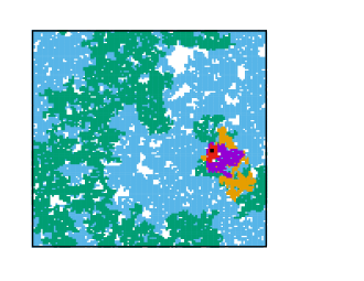
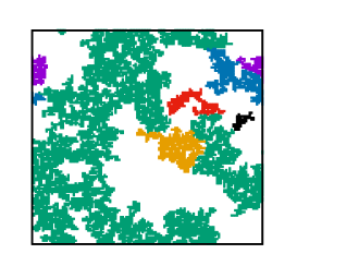
In the following, we shall call each epidemic starting from $i$ a “wave”, and $h$ its height. Since the supports ${\cal C}_{h}$ of successive waves are nested, we obtain in this way a landscape with a single mountain of peak height $h_{i}$, and “terraces” of heights $h<h_{i}$ (see Fig. 1). Each terrace is just

$$\Delta{\cal C}_{h}\equiv{\cal C}_{h}\setminus{\cal C}_{h+1}.$$ (2)

The part of the lattice which was not even touched by the first wave is called the zeroth terrace with height $h=0$ Note5 .

(b) Finding viable clusters attached to other points: After we have obtained the largest cluster attached to $i$ we could pick another site $j$ (either randomly or by going systematically through the lattice), and repeat the same process. To find the largest viable cluster on the entire lattice ${\cal C}_{\rm max}$, we would then have to repeat this for all sites. But this would be extremely time consuming. We are interested in the phase transition where ${\cal C}_{\rm max}$ becomes macroscopic in the limit $N\to\infty$. This happens at a critical value $q_{c}$ of $q$ which is far above the critical value for single epidemics. Thus for all seeds the first few waves will most likely be huge, and most of the CPU time is spent for finding out clusters which overlap so much that they are nearly identical and cover nearly the entire lattice. The resulting CPU time would then be roughly ${\cal O}(N^{2})$.

Fortunately, there is no need to use this brute force algorithm. Let us consider the system of waves and terraces for the second seed $j$. Since the entire lattice is covered by terraces from the first seed $i$, we can assume that $j$ is on a terrace of some height $h\in\{0,1,\ldots h_{i}\}$. If the height were equal to $h_{i}$, $j$ would be part of the first cluster. Thus we can assume that $h<h_{i}$. If $h=0$, then $j$ is not connected to $i$ by the red bonds, and thus any viable cluster attached to $j$ must be contained in the zeroth terrace $\Delta{\cal C}_{0}$. Otherwise (if $0<h<h_{i}$) we can use

Lemma 1: If $h>0$, the first $h$ waves starting from $j$ cover exactly the same clusters ${\cal C}_{h^{\prime}}$ (with $h^{\prime}\leq h$) as the waves starting from $i$.

Proof: The proof is by induction and uses the fact that each wave just covers all sites on a given network that can be reached from the seed, where each of these networks is the subgraph of the original network reached by the previous wave. First of all, it is clear that the lemma holds for $h=1$, because ${\cal C}_{1}$ is the set of all points on the original network that are connected to the seed by red bonds. Since the two seeds are connected by red bonds due to the assumption that $h>0$, any point $k$ connected to $i$ must also be connected to $j$ and vice versa. Let us now assume that for some $h^{\prime}<h$ the clusters attached to $i$ and $j$ are the same. Then we can use exactly the same argument, just replacing the original network by ${\cal C}_{h^{\prime}}$ and using the appropriate color of the bonds.

Thus we do not need to follow the first $h$ waves starting from $j$, and we can immediately start with wave $h+1$. In doing so, we can use also another important simplification because of

Lemma 2: Assume that point $j$ is on a terrace of height $h<h_{i}$. Then the entire next wave is confined to this terrace.

Proof: For the proof we have to show that the next wave neither spills over to the lower terrace, nor to the higher.
For the first part we can assume $h>0$. Assume now that the wave actually does spill over, i.e. there exists a point $k$ which is connected to $j$ but is on a lower terrace. This point would not be connected to $i$ on any terrace with $h^{\prime}>=h$, while $j$ is. This cannot be.
For the second part we assume for the moment that the wave spills over to a higher terrace, i.e. there exists a point $k$ which is connected to both $k$ and $i$. But since $j$ is not on this higher terrace (i.e. is not connected to $i$), this cannot be either.

Thus when building the terraces for site $j$ we can restrict ourselves to waves for which all boundaries of the terraces generated by the first seed form obstacles which cannot be crossed. It is easy to see that this generalizes also to all later seeds, when the landscape is made up be any number of terraces and boundaries between them:

Proposition 1: If a seed $j$ happens to be on any terrace with a height $h$ which is not a local maximum (i.e., $j$ is not in a locally maximal viable cluster), then all previous wave boundaries form obstacles for all avalanches starting at $j$ which have to be followed in order to get the viable cluster attached to $j$.

The proof uses the same arguments as above. We just have to realize that successive waves that started from later and later seeds are just distinguished by more and more restricted subsets of the original network to which they are confined. Whatever these subsets are, the above proofs go through without modification.

It should now be clear why we call this procedure an SOS type growth process. As in any SOS model, we have a rough landscape and the growth of this landscape proceeds by localized events, each of which builds a hierarchy of nested terraces. As in surface diffusion problems with strong Schwoebel barriers, these events cannot spill over the boundaries set by previous events.

Notice that neighboring terraces belonging to different seeds can have the same height. Also in this case, their boundaries cannot be crossed by later waves from other seeds. To implement this restriction we either use an additional marker for each site which tells us the seed to which it belongs; or, alternatively, when each wave is finished, we cut all bonds connecting the wave with its complement. Both methods allow us to prevent the waves from spilling over the terrace boundary, without modifying the dynamics inside any terrace. Also, when we start with a new seed $j$, we choose the color of the first wave according to the landscape height $h$ at this seed, and we count subsequent heights by adding to this $h$. Since now every site $i$ is “infected” precisely by $h_{i}$ waves, it follows that the algorithm has time complexity $N\langle h\rangle$, where $\langle h\rangle$ is the average height. This estimate holds for arbitrary graphs, provided all node degrees are bounded.

Before we show numerical results, we present also a second proposition which we did not find useful for numerics, but which could be very useful for mathematical treatments.

Proposition 2: The final landscape and the system of all terrace boundaries is independent of the sequence by which the seed points are chosen.

Thus the landscape is not a property of the realization of the algorithm (which involves an arbitrary choice of going through all seeds), but is an inherent property of the network. In essence, it says that the growth of the surface is Abelian in a similar way as the Bak-Tang-Wiesenfeld sand pile model is Abelian Dhar .

For the proof we can use the fact that any permutation of sites can be written as a product of pairwise transpositions. We thus need to show only that it does not matter whether we first take seed $i$ and then seed $j$ or the inverse. But this follows from the arguments in the proofs of Lemma 1 and 2.

We should add that we checked both propositions also numerically, finding perfect agreement.

Finally, we should point out how our sequences of waves are related to the failure cascades of Buldyrev and to other algorithms proposed for them. One essential difference is that we do not demand that the cluster surviving the cascade is always the maximal one. Rather, the maximal cluster is determined at the end, when all viable clusters are known. This simplifies the algorithm of course considerably. Also the complexity of the algorithm of Hwang is related to the fact that they always follow the largest viable cluster. This precaution is not taken in the algorithm of Schneider , where it is assumed that a cluster which starts large at the beginning of the cascade is not overtaken later by one which starts smaller. This is true for sparse tree-like graphs (whence their algorithm gives correct results), but it is not true in general. Related to this is the absence of the notion of ‘seed’ or ‘source’ in these algorithms. While in our algorithm each ‘cascade’ gives just one cluster arbitrarily picked by the seed, the cascades studied in Buldyrev are constructed so as to lead always to the largest cluster. As a consequence, the average cascade length in Buldyrev is in our interpretation essentially the average height of the largest viable cluster, which is in general (but not always?) an upper bound for the average surface height.

A last difference between our algorithm and that of Buldyrev is that we always start our ‘cascades’ from the full (undamaged) system, while the cascades of Buldyrev are supposed to be triggered by (small and successive?) damages, starting from an already partially damaged system. On the other hand, our algorithm shares with that of Buldyrev that it does not deal – in contrast to what is suggested in Buldyrev – with any real dynamics. Both algorithms deal with pseudodynamics in a fictitious time, and should not be confused with actual cascading processes going on in real time.

III Applications

III.1 Erdös-Rényi Networks

We first apply our algorithm to duplex ER networks where both layers have the same average degree $z=\langle k\rangle$. In this case it is known from Son1 ; Son2 that the generating function formalism of NSW ; Newman gives the exact threshold and the exact dependency of the order parameter on $\langle k\rangle$. Thus it can be used to test the accuracy of the algorithm. On the other hand, we shall also use it to find the average height of the landscape and the average height of its maxima (i.e., of the largest clusters). The latter is just the average cascade life time in the interpretation of Buldyrev . Since during the cascades the clusters are supercritical, it is not a priori clear whether the mean field theory arguments used in Buldyrev to derive a scaling law for this life time are exact. To make a short summary, we will find that the algorithm works perfectly, but the mean field arguments of Buldyrev for the life time seem to be to be only approximate. This implies that also the arguments of Buldyrev in favor of the percolation threshold value have to be taken with care – although they give the correct result – because they rely on the assumed mean field cascade dynamics.

Figure 2: (color online) Order parameter (density of giant viable clusters) for ER networks plotted against the average degree $z$. The continuous curve is the prediction of Eq. (3), while the points are from simulations with $N$ ranging from $2^{14}$ to $2^{26}$. For $S<0.511700...$ the theoretical curve is strictly vertical, while it has square-root behavior above.

Figure 3: (color online) Differences between the data points and the theoretical curve in Fig. 2. To enhance the region $z\approx z_{c}$, the data are plotted against $z-z_{c}$ on a logarithmic axis.

Figure 4: (color online) Differences between the data points for $z=z_{c}$ and the theoretical value 0.511700 towards which they should converge for $N\to\infty$. We see indeed a straight line on a log-log plot, which leads to Eq. (5).

We consider networks with $N=2^{m}$ nodes, with $m=4,\ldots 26$. The average degree was varied in the range 1.9 to 3.2. The critical point is known in this case to be at $z_{c}=2.45540748\ldots$. The number of realizations simulated at $z_{c}$ varied from $\approx 10^{8}$ for $N=1024$ to $>600$ for $N=2^{26}$.

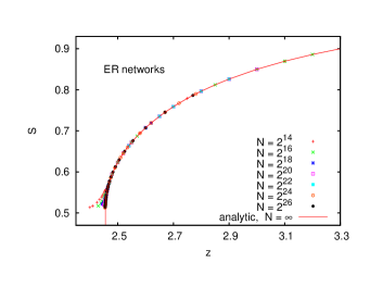
The density of the giant viable cluster on an infinite ER network is given by the largest solution of the equation Son1

$$F(S)\equiv S-(1-e^{-zS})^{2}=0.$$ (3)

It vanishes for $z<z_{c}$, and has both a jump and a square root singularity at $z=z_{c}$,

$$S=0.511700+a\sqrt{z-z_{c}}+...\quad{\rm for}\quad z>z_{c}.$$ (4)

For finite $N$ there are of course corrections, the analytic form of which is not known.

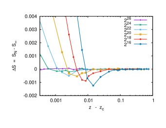
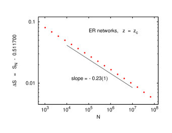
Numerical results for $S_{N}$, the average relative size of the giant cluster on a graph of size $N$, are given in Figs. 2 to 4. Actually, in these plots we show (in contrast to analogous plots in the next subsections) $S_{N}$ conditioned on realizations which do have a giant cluster. Notice that all other clusters are extremely small (for $N>2^{20}$ we found only clusters of sizes 1 or 2 apart from the giant one, and even for $N=1024$ the largest non-giant clusters had sizes $<8$), thus it is straightforward to identify giant clusters, except for $N<10^{3}$. In Fig. 2 we show $S_{N}$ versus $z$. Since this gives a perfect agreement with Eq. (3) except for $z$ extremely close to $z_{c}$, we plot in Figs. 3 and 4 differences between analytical and numerical results for a more sensitive comparison. From Fig. 3 we see that the finite-$N$ corrections are indeed not monotonic, as one might have suggested from Fig. 2, but they decrease fast with $N$. For $N=2^{26}$, the deviations from the theory for $N=\infty$ are $<10^{-4}$ for all $z$ except extremely close to $z_{4}$, which is just the level of statistical errors. Thus we verified with very high precision that our algorithm gives results in agreement with Eq. (3) not only near the critical point, but also for all $z>z_{c}$. The agreement at $z=z_{c}$ is checked in Fig. 4, where the differences $\Delta S_{N}=S_{N}-S_{\infty}$ are plotted against $N$. We see a perfect scaling law

$$\Delta S_{N}\sim N^{-\alpha}\quad{\rm with}\quad\alpha=0.23(1).$$ (5)

To our knowledge there is no theoretical prediction for $\alpha$. For $z>z_{c}$, Fig. 3 is consistent with $\Delta S_{N}\sim N^{-\alpha}\phi[(z-z_{c})N^{1/2}]$, but the data are too noisy make a strong claim for it.

Figure 5: (color online) $P_{N}(z)$, the probability to have a giant viable cluster on an ER network of size $N$, plotted against $(z-z_{c})N^{1/2}$.

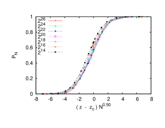
There also seems to exist no prediction for the behavior of $P_{N}(z)$, the chance that there exists a viable giant cluster on a network of size $N$. In analogy to ordinary percolation we expect that this is a step function in the limit $N=\infty$, i.e. $P_{\infty}(z)=\Theta(z-z_{c})$, but the behavior for finite $N$ is non-trivial. In Fig. 5 we plot $P_{N}(z)$ against $(z-z_{c})N^{1/2}$. We see that all curves become essentially parallel, i.e. we have a data collapse apart from a correction to scaling that leads to a shift of the effective transition point towards higher $z$ as $N$ increases.

Figure 6: (color online) Average “surface” heights (i.e. cascade life times) for three network sizes, plotted against $z$. While the collapse of the three curves for $z\ll z_{c}$ is easy to understand, the behavior at larger $z$ is more interesting.

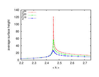
“Surface” heights (i.e. average cascade life times) measured in these simulations are discussed in the next figures. In Fig. 6 we show for three different network sizes how the average surface heights, averaged over all nodes, depend on $z$. As expected, they are small for $z\ll z_{c}$ and become quickly independent of $N$: For small $z$ there are only small clusters to start with, and the cascades terminate quickly. For $z\gg z_{c}$ there are only small holes in the viable clusters and they also are quickly identified, whence the cascades terminate soon also in this regime. It is less obvious why the heights do not seem to become independent of $N$ as $z$ becomes very large. The most conspicuous feature of Fig. 6 is, however, the sharp peaks developing at $z=z_{c}$ as $N$ increases. Figures 7 to 9 deal with several aspects of these peaks.

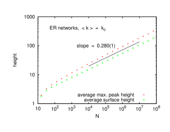
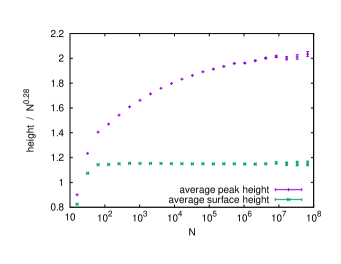
Heights of the peaks (more precisely the average surfaces heights at $z=z_{c}$; the peaks occur slightly to the left of $z_{c}$) are shown in Fig. 7. In the same figure we also show, in addition to the average surface heights, the (averages of the) surface peaks, i.e. the highest points in the “landscapes”. At least for ER networks (where we have no large viable clusters apart from the giant ones) we expect these peak heights to be precisely the average durations of the cascades studied in Buldyrev (see also Zhou ). We see from Fig. 7 that the average heights show a perfect scaling,

$$\langle h\rangle\sim N^{\gamma}\;,\qquad\gamma=0.280(1).$$ (6)

In contrast, the peak heights in the landscape seem to increase with the same asymptotic power law, but with large finite-$N$ corrections. The latter are presumably the usual bias corrections in extremal properties evaluated over finite domains. One has similar (logarithmic?) corrections e.g. in the average size of the largest cluster in subcritical (ordinary) percolation on finite lattices.

Eq. (6) is in clear contradiction to the result $h_{\rm peak}\sim N^{1/4}$ obtained in Buldyrev by mean field arguments which do give also the correct Eq. (3) for the cluster size and the exact value of $z_{c}$. This is rather puzzling. One might try to explain it by noting that the value of $z_{c}$ depends only on clusters which are barely viable, and thus the local tree-likeness of sparse ER networks should be sufficient – while the cascade dynamics deals always with supercritical clusters. But then it is not clear why Eq. (3) should be correct also for $z>z_{c}$, which we took great pain to verify. Notice that the violation of the mean field prediction seen in Fig. 6 is not related to the observations in Zhou . In that paper it was shown that an apparent violation of mean field theory is observed, if one does not use the true critical value of $p_{c}$ in the analysis, but an effective one that changes from realization to realization. In our analysis, $p_{c}$ is always the true critical point. In any case, our value of $\gamma$ disagrees both with the mean field exponent 1/4 obtained in Buldyrev and with the exponent 1/3 proposed in Zhou , which was based on simulations of much smaller systems with much lower statistics.

Figure 7: (color online) (a) Average “surface” heights at $z=z_{c}$ plotted against networks network sizes on a log-log plot, and average values of the peaks in each surface. Both curves clearly disagree with the scaling $\propto N^{1/4}$ proposed in Buldyrev , but give rather an exponent $0.280(1)$; (b) The same data, but divided by $N^{0.280}$.

Figure 8: (color online) Log-log plots of $\langle h\rangle$ against $|z-z_{c}|$. The straight lines indicate power laws which we claim to hold in the limit $N\to\infty$.

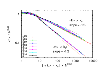
The “wings” of the peaks seen in Fig. 6 are studied more closely in Fig. 8, where we plotted the heights (on a log scale) against $\log|z-z_{c}|$. For the subcritical regime $z<z_{c}$ we clearly see a power law with exponent $1/2$, in perfect agreement with Zhou (notice, however, that we could not confirm the other scaling laws suggested in Zhou ). We did not try to derive this analytically, but doing this should not be difficult. For $z>z_{c}$ the situation is less clear, but it seems that for large $N$ a power law with exponent $1/3$ emerges, even if corrections are large for finite $N$.

Figure 9: (color online) Data collapse plots of re-scaled surface heights $\langle h\rangle/N^{\gamma}$ against $(z-z_{c})N^{2\gamma}$ with $2\gamma=0.56$ (panel a) and against $(z-z_{c})N^{0.5}$ (panel b). Neither plot is fully satisfactory, but in spite of the bigger overall discrepancies we claim that panel (b) gives the correct collapse in the critical region.

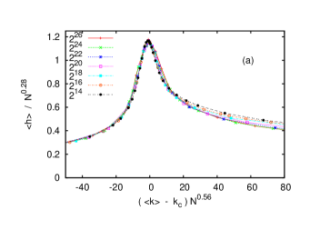
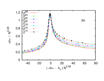
The two panels of Fig. 9 show finally two attempts to produce a data collapse for the entire critical region. In panel (a) we plotted $\langle h\rangle/N^{\gamma}$ against $(z-z_{c})N^{2\gamma}$. This gives us a perfect data collapse subcritically. In the critical and supercritical regions the plot does not look too bad either, but a closer inspection shows that it is indeed unacceptable. In contrast, in panel (b) we plotted the data against $(z-z_{c})N^{0.5}$. This time the collapse is very poor in the wings, but we get a very good collapse in the critical region – apart from the same shift of the effective critical point also seen in Fig. 5. Notice that the variables on the x-axis in Figs. 5 and 9 are the same.

III.2 2-dimensional Lattices

We next study 2-d square lattices of size $L\times L$, with $32\leq L\leq 32768$ and with helical boundary conditions Note4 . The two sets of links are different (randomly chosen) subsets of nearest neighbor bonds. For each of them we include a bond with probability $p$ and exclude it with probability $1-p$. In addition, we can also make a fraction $q$ of sites inaccessible. For $p=1$ and $0<q<1$ the red and green links coincide, and we simply deal with site percolation with control parameter $q$. On the other hand, if $p<1$ and $q=1$, the sets of red and green links overlap. Each one of them would define a bond percolation problem, and the viable clusters are subsets of intersections of red and green percolation clusters.

For $p<1$ and $q<1$, the single color problems would correspond to mixed site-bond percolation. We studied also that case, because the problem was originally formulated in Buldyrev as a robustness problem for network break-down under successive node removal. In that interpretation one needs $p<1$ for having a multiplex network, and $q<1$ due to node removal. Actually, however, the problem just becomes more complicated by having both $p$ and $q$, without adding any conceptual advantage. If one wants to interpret results obtained with $q=1$ (i.e. with an undiluted lattice) in terms of robustness against damage, then one simply has to implement the damage not as site removal, but as bond removal.

In the following we shall present results for $q=1$ and varying $p$ (because this is conceptually the simplest), and for $p=0.6$ and varying $q$. The latter was done in order to compare with the results of Son1 ; Berezin3 ; Son3 . It leads to $q_{c}\approx 0.96$. In neither case the exact critical point is known. The total number of realizations were in both cases between $>10^{8}$ for the smallest, and several thousand for the largest lattices.

Figure 10: (color online). Data collapse plot for the size of the largest viable cluster on 2-d lattices with $p=0.6$. The only perceptible deviation from a perfect collapse is at very large values of $q$, where the data for $L=256$ and for $L=512$ are systematically too high, due to finite-size corrections.

Figure 11: (color online). Log-log plot of $S$ against $q-q_{c}$, demonstrating the power law $S\sim(q-q_{c})^{\beta}.$

Figure 12: (color online) Log-log plot of $L^{2}S/L^{91/48}$ against $L$, for eight values of $q$ close to $q_{c}$. The power $91/48=1.8958\ldots$ was chosen, because it is the fractal dimension of the incipient giant cluster in critical OP. Thus any deviation of the critical curve from a horizontal line indicates that the present model and OP are in different universality classes.

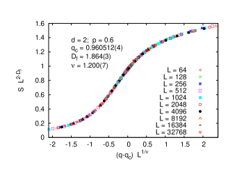
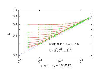
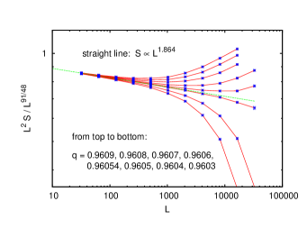
Results for $p=0.6$ are shown in Figs. 10 to 12. In Fig. 10 we show a data collapse similar to the corresponding plots in Son1 ; Berezin3 . We see a perfect collapse, if we use $q_{c}=0.960512(4)$ and $\nu=1.2$. These values agree roughly with those proposed in Son1 , but are very different from those in Berezin3 . In particular, we would obtain a very bad collapse (for any value of $\nu$), if we would use $q_{c}=0.9609$ as proposed in Berezin3 . Also, we would obtain a very bad collapse (for any value of $q_{c}$), if we would take for $\nu$ the value 4/3 as in ordinary percolation. We should point out that the largest lattice sizes studied in Berezin3 were only $3000\times 3000$.

Supercritical data are plotted as $S$ against $q-q_{c}$ on a log-log plot. For large $L$ and $q$ not too close to $q_{c}$ we expect a power law

$$S\sim(q-q_{c})^{\beta}.$$ (7)

This is indeed nicely confirmed, with $\beta=0.163(2)$. Notice that this is perfectly consistent with the scaling relation $D=2-\beta/\nu$, but is again different from the value for OP. Notice also that the power law holds only for $q-q_{c}<0.01$. For larger distances from the critical point, corrections would be needed.

Finally, we show in Fig. 12 a log-log plot of $S$ against $L$. To make the plot more significant, we actually divides $S$ by the power of $L$ expected for OP, so that the critical curve would be horizontal if the present model were in the OP universality class, as claimed in Berezin3 . The dashed straight line indicates the power law consistent with the previous two figures.

Figure 13: (color online). Data collapse plot for the variance of the size of the largest viable cluster on 2-d lattices with $q=1.0$, plotted against rescaled values of $p-p_{c}$.

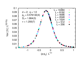
Essentially the same results were obtained when we kept $q=1$ fixed (i.e., no sites were deleted), and $p$ was allowed to vary. This time we studied only lattices with sizes up to $16384\times 16384$, but with higher statistics. The critical point is now $p_{c}=0.576132(5)$. All critical exponents are compatible with these given above, and have roughly the same error bars. The main difference with the case $p=0.6$ is that now corrections in the far supercritical region do not make the curves in the log-log plot of $S$ against $p-p_{c}$ turn up (as in Fig. 11), but make then turn slightly down. To avoid duplication we do not show the dame plots as for $p=0.6$, but we do show a data collapse plot for the variance (“susceptibility”) of $S$.

Figure 14: (color online) Average SOS landscape heights for 2-d lattices with $q=1$, plotted against $p$.

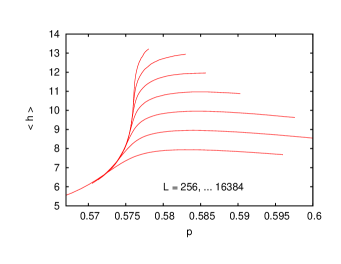
Average landscape heights are shown in Fig. 14. We see a behavior rather different from that seen in Fig. 6 for ER graphs. While the latter showed a very sharp peak at the critical point, whose height and sharpness both increased with powers of the system size, we have now a very wide bump far in the supercritical region, whose width does not seem to depends on $L$ at all, and whose height increases logarithmically with $L$. The most conspicuous feature of Fig. 14 is that the slopes at $p=p_{c}$ become increasingly steeper with $L$, roughly as

$$\frac{d}{dp}\langle h\rangle\sim L^{0.7}\quad{\rm at}\quad p=p_{c}.$$ (8)

In contrast to the ER case, where we could find a decent scaling behavior of $\langle h\rangle$ near the critical point, we were unable to find any convincing scaling in the present case.

Before leaving this subsection, we should mention that all scaling laws and critical exponents found in this subsection were also found in a very different microscopic realization of the 2-d lattice model discussed in subsection III.F.

III.3 3-dimensional Lattices

For lattices with $d>2$ we made only simulations without site decimations, i.e. we always used $q=1$.

In Son1 , simulations of very small lattices had suggested that the transition is also for 3-dimensional lattices continuous and not in the OP universality class. This is important, since it could be argued that the transition is continuous for $d=2$ because there the two sets of links necessarily overlap strongly, and in that case the transition can be continuous even on ER networks Parshani . In three dimensions, this overlap is much reduced.

Figure 15: (color online) Log-log plot of $L^{3}S/L^{D_{OP}}$ against $L$, for eight values of $p$ close to $p_{c}$. Here, $D_{OP}=2.523(1)$ is the fractal dimension in three-dimensional OP Lorenz ; Deng . Indeed, since we used helical b.c. where the number $N$ of lattice sites was always a power of 2, some of the lattices were not strictly cubes. In these cases, $L$ was nevertheless defined as $L=N^{1/3}$, even if this was not an integer. The values of $p$ are (from top to bottom) $0.357,0.3568,0.35673,0.35670,0.35668,0.35665,0.3566,0.3565$.

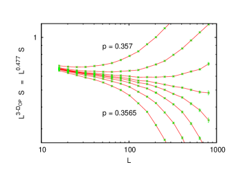
Our present simulations show that the transition is indeed continuous, but the deviations from OP scaling are much smaller than found in Son1 . In Fig. 15 we show a log-log plot of rescaled infinite cluster sizes against $L$ for eight values of $p$ close to $p_{c}$. Here $L$ is defined as $L=N^{1/3}$, where $N$ is the number of lattice sites. Since we used helical b.c. where $N$ was always a power of 2, the so defined $L$ is not always an integer, and the lattices are not always exact cubes. This has however no noticeable effect on the scaling. Since we want to compare with OP, where $L^{3}S\sim L^{D_{OP}}$ with $D_{OP}=2.523(1)$ Lorenz ; Deng , we multiply the data with the corresponding power of $L$. Thus we expect one curve (the critical one) to be horizontal, if and only if the present model is in the universality class of OP. We see that the most straight curve has a slightly negative slope. This gives $p_{c}=0.356707(4)$ and

$$D_{f}=2.475(8)$$ (9)

(the estimate of Son1 was 2.40(1)), which would nominally indicate that the present model is in a different universality class. As we shall see, however, there are important corrections to scaling. Thus the error in this estimate may be severely underestimated.

Figure 16: (color online). Data collapse plot for the size of the largest viable cluster on 3-d lattices. In contrast to the 2-d case we now have huge corrections to scaling in the supercritical region.

Figure 17: (color online) Average SOS landscape heights for 3-d lattices, plotted against $p$.

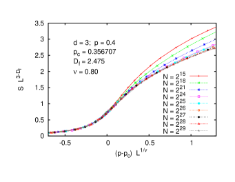
These corrections to scaling are most clearly seen in a data collapse plot, see Fig. 16. In contrast to the analogous plot for $d=2$ in Fig. 10, we see now huge deviations in the supercritical region. Nevertheless, in the critical and under critical regions the collapse seems to be very good. Notice that we used here the values for $D_{f}$ and $p_{c}$ obtained from the previous plot. For the correlation length exponent we obtain $\nu=0.80(3)$, which is significantly lower that the value $0.8734$ obtained fro OP Deng . Hyper scaling finally gives $\beta=(d-D_{f})\nu\approx 0.42$, in agreement with OP. In summary it seems that corrections to scaling were severely misjudged in Son1 , and we cannot exclude that the model is in the OP universality class for $d=3$.

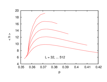
A reason for it to be not in the OP universality class is, of course, the divergence of the surface height when $L\to\infty$. This is clearly seen from Fig. 17, where we find the same logarithmic increase as in $d=2$, and a power law for the slope at $p=p_{c}$ as in Eq. (8), but with exponent $\approx 0.82$.

III.4 4-dimensional Lattices

Figure 18: (color online) Average SOS landscape heights for 4-d lattices, plotted against $p$.

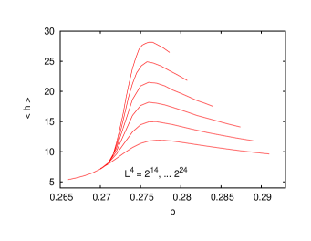
As a first result we show the average surface heights, see Fig. 18. Their behavior is very similar to those in two and three dimensions: For any $N=L^{4}$ their maxima occur in the supercritical region, and their heights increase logarithmically with $L$. Also, the slopes $d\langle h\rangle/dp$ diverge for $L\to\infty$ with a power law, again with power slightly smaller than one (our best estimate is $\approx 0.9$).

Figure 19: (color online) Average density of the largest viable cluster on 4-d lattices with $N$ sites, plotted against $p$. The sharpness of the kink at $p\approx 0.2715$ increases with $N$.

Figure 20: (color online) The same data as in Fig. 19, but plotted such that the collapse onto a single curve near the critical point.

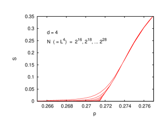
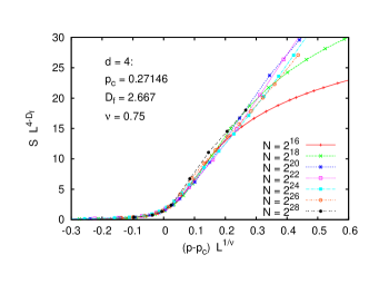
In contrast to this, the behavior of the order parameter is completely different. In Fig. 19 we show plots of $S$ versus $p$, for lattice sizes with $N=2^{16},2^{18},\ldots 2^{28}$, corresponding to $L=16,\ldots 128$. We see clearly a continuous transition, but with order parameter equal to (or at least very close to) $\beta=1$. This would indicate that $d=4$ is the upper critical dimension, in striking contrast to OP, where $d_{u}=6$. An attempt to collapse the data according to standard FSS leads to Fig. 20, and to $D_{f}\approx 8/3$ and $\nu\approx 3/4$. These would not correspond to any known mean field theory, but we should be aware that we should expect logarithmic corrections, if indeed $d_{u}=4$. The poor quality of the collapse might indicate that such corrections are indeed present, but with our present data we have no chance to estimate them in detail.

Figure 21: (color online) Log-log plot of the integrated mass distribution of 4-d viable clusters at $L=128$ and $p=0.27145$. The straight line has slope $-3/2$ as predicted from standard scaling laws, accepting the exponents found in Fig. 20.

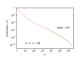
Finally, we show in Fig. 21 the integrated mass distribution on a large lattice for $p\approx p_{c}$. If usual FSS would hold, we would expect a power law

$$p(m)\sim m^{1-\tau}$$ (10)

with

$$\tau=1+d/D_{f}\;.$$ (11)

Inserting here our numerical result $D_{f}=8/3$ gives $\tau=2.5$. The data show a very rough power law, with large deviations at intermediate mass values, but the distribution agrees surprisingly well with Eq. (10) for large masses.

III.5 5-dimensional Lattices

Figure 22: (color online) Average density $S$ of the largest viable cluster on 5-d lattices with $N$ sites, plotted against $p$. Notice that we averaged here over all runs (even if they did not have a giant viable cluster), while the averages in subsection III.A (e.g. Fig. 2) were done only over runs that did have a giant cluster.

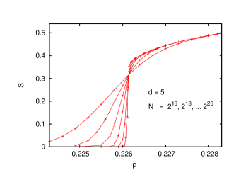
If the present problem represents indeed a new universality class with upper critical dimension $d_{u}=4$, then the behavior in $d=5$ should be essentially the same as for $d\to\infty$, and in particular as on ER graphs. To verify this we show first (in Fig. 22) the order parameter $S$ (the density of the largest viable cluster) as a function of $p$. We see that the curves for different sizes $N$ intersect indeed in a single point, with $p_{c}=0.22614(1)$ and $S_{c}=0.31(1)$. This jump of $S$ is a clear sign of a discontinuous transition, although the rise of $S$ for $p>p_{c}$ indicates that the transition is also, as for ER networks, hybrid.

Figure 23: (color online) Average SOS landscape heights for 5-d lattices, plotted against $p$.

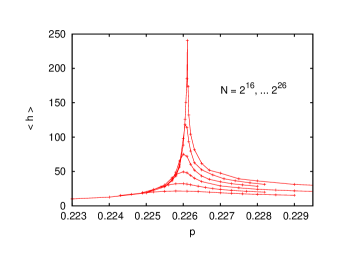
The same conclusion is reached by looking at surface heights (Fig. 23), which display the same sharp peak as for ER networks. Also, the heights of the peaks increase with roughly the same power of the system size ($h_{\rm max}\sim N^{0.30(2)}$), not logarithmically as on lattices with $d\leq 4$.

Figure 24: (color online) Log-log plot of the integrated mass distribution of finite 5-d viable clusters at $N=2^{26}\;(L\approx 37)$ and $p=0.22615$. The straight line indicates the scaling of finite but large viable clusters.

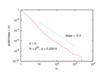
On the other hand, the statistics of finite viable clusters is markedly different from that for ER networks. There, apart from the giant viable cluster all other clusters are of size one in the $N\to\infty$ limit Buldyrev , and for the system sizes studied in the present work most of them have sizes one or two. On five-dimensional lattices, however, the distribution of finite viable clusters is non-trivial. The average mass of the second-largest clusters peaks for $p_{c}-p\sim L^{-2}$, and the peak height increases roughly as $L^{2}$ (both of these exponents are very crude estimates). Moreover, the mass distribution of the finite clusters shows rough scaling, $p(m)\sim m^{-2.4}$ at $p=p_{c}$ (see Fig. 24).

III.6 Cross-over to Mean Field Theory via Long Range Links on 2-d Lattices

III.6.1 General Remarks: Long Range Connectivity vs. Long Range Dependency

In general, there are two main ways how the anomalous behavior of critical phenomena seen on low dimensional lattices can cross over to mean field theory. One is by increasing the dimension, the second is by making the theory more and more non-local. In the present model we found that the transition via dimension increase is very non-standard, by showing first a transition to a mean field critical point (at $d=4$), which is then replaced by a first order transition at $d>4$. In view of this, it is of interest to check what mechanism(s) are at play when one makes the model more and more non-local.

In the interpretation as multiplex networks (where any interdependent node pairs are joined into a single node) adopted in this paper, the most natural way to do this is by increasing the lengths of the (“connectivity”) links. In analogy with standard critical phenomena one would expect that the model stays in the same universality class as long as the characteristic length of the bonds are finite, and crosses over to mean field theory only when this length becomes infinite, e.g. by having power-behaved link length distributions (see, e.g., Grass2013 ; Grass2013b ). One cannot rule out, however, that there exists a tricritical point at some finite length.

In the original interpretation of Buldyrev as a model with distinct connectivity and dependency links, one can make either of them long ranged, or both. In Li-Bashan ; Berezin2 ; Danziger it is assumed that nodes are located on 2-d lattices with nearest neighbor connectivity links, while dependency links become long ranged. This is presumably not very realistic in most applications: Since dependency links are much more crucial than connectivity links, one would assume that they are the shorter ones in any realistic natural network. In the following we shall just make some comments on the model of Li-Bashan ; Berezin2 ; Danziger , and leave the more natural model of multiplex networks with long range connectivity links to a future publication.

III.6.2 Random Dependency Links

As in Li-Bashan , we first discuss the case where the dependency links are completely random (while, as we said, the connectivity links are the nearest neighbor bonds). The transition is obtained by varying the site occupancy $q$ of one of the two dependency partners (i.e., any pair of dependency partners is present with probability $q$), and keeping all dependency links (i.e., $p=1$). This is the $r\to\infty$ limit of the model discussed in the next sub-subsection. Following cascades, it was shown in Li-Bashan that the transition is first order in this limit, and closed formulas were given for the threshold $q_{c}$ and for the density of the viable cluster at threshold.

As in the case of random locally tree-like graphs Son1 ; Son2 , these formulas are indeed obtained more easily from consistency considerations without reference to any cascade dynamics. Let us denote by $S_{\rm OP}(p)$ the order parameter (i.e. the density of the infinite cluster) in ordinary site percolation with site occupancy $p$ (the subscript “OP” stands for ‘ordinary percolation’). Let us now consider the percolation of one type of nodes, say of nodes of type A. Since dependencies are completely random, they are not correlated with the (non-trivial) order parameter fluctuations, and they just mean that a finite density of A nodes will be killed by not having a viable dependency partner. This fraction is exactly the same as the fraction of B nodes that are killed because they have no viable A partner. As a result, starting with occupancy $p$ in ordinary site percolation leads to the same order parameter as starting with occupancy $q$ in the dependency model, provided that Li-Bashan

$$q=p\times p/S_{\rm OP}(p)\;,$$ (12)

and $S_{\rm OP}(p)$ is also the density of the viable cluster when starting with $q$. Plotting the r.h.s. of Eq. (12) versus $p$ gives a convex function (see Fig. 25), the minimum of which is the critical value of $q$,

Figure 25: (color online) Plot of $p^{2}/S_{\rm OP}(p)$ versus $p$. The points are most precise near the minimum of the curve, where each point is obtained from $\approx 10^{3}$ lattices of size $32768\times 32768$. The statistical errors of these points are smaller than their sizes.

$$q_{c}=\min_{p}p^{2}/S_{\rm OP}(p)=0.682892(5)$$ (13)

with

$$p^{*}=\arg\min_{p}p^{2}/S_{\rm OP}(p)=0.6418(2),$$ (14)

and $S_{c}\equiv S_{\rm OP}(p^{*})=0.6031(2)$ is the density of the giant viable cluster at threshold. The numerical values are in good agreement with the less precise estimates of Li-Bashan .

Figure 26: (color online) Average density $S$ of the largest viable cluster on 2-d lattices with random dependency links and dependency links between nearest neighbors, plotted against $q$. In the main figure, averages are taken over all runs (even they did not lead to a giant viable cluster, while the inset shows averages restricted to runs with giant viable clusters.

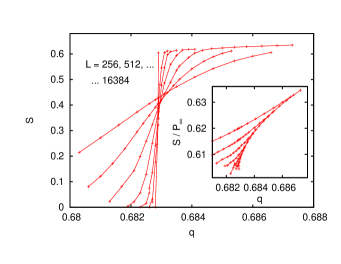
The existence of a first order transition with these parameter values was also confirmed by direct simulations. In Fig. 26 (main plot) we show the order parameter (the density of the largest cluster, averaged over all runs) plotted against $q$. Densities obtained by averaging only over those runs which did lead to a giant viable cluster are shown in the inset. As in the ER case, it was trivial to distinguish between runs with and without giant clusters, because all non-giant clusters had sizes 1 or 2 (except on very small lattices, where also clusters of size 3 were seen). Figure 26 confirms not only the values of $q_{c}$ and $S_{c}$, but it also shows that the transition is hybrid, because the slope at threshold is infinite. The latter is a direct consequence of the fact that the minimum in Fig. 25 is quadratic.

Figure 27: (color online) Log-log plot of average SOS surface heights at $q=q_{c}$ for interdependent networks on square lattices with random dependency links. The straight line indicates a power law with exponent 0.556.

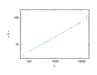
The dependence of the average SOS surface heights on $q$ and on $N=L^{2}$ is also very similar to that for ER networks. As functions of $q$ they show peaks that become narrower and higher with increasing $L$, and the peak values (more precise, the values at $q=q_{c}$) show a power law

$$\langle h(q_{c})\rangle\sim L^{0.556(10)}.$$ (15)

(see Fig. 27). This is in qualitative agreement with findings by D. Zhou (quoted in Danziger ), who obtained however an exponent 0.44, in clear disagreement with our value 0.556. On the other hand, the scaling $\langle h(q_{c})\rangle\sim N^{0.278(5)}$ is the same as that for ER networks (see Eq. (6)).

III.6.3 Intermediate-Range Dependency Links

Irrespective of all details, the results of the last sub-subsection show unambiguously that the transition is first order in the limit of infinitely long dependency links and nearest neighbor connectivity links, and the transition occurs roughly at $q\leq 0.7$. This should be remembered if we now consider, following Li-Bashan ; Berezin2 , dependency links with intermediate range.

In Li-Bashan ; Berezin2 the dependency links were random vectors ${\bf x}=(x,y)$ with $||{\bf x}||<r$ in the maximum norm. it was found that the model stays second order, as long as $r<8$. At $r=r^{*}\approx 8$ the transition becomes first order, and for $r>8$ there are claimed to be two first order transitions with a metastable phase in between. The percolation is again implemented as site percolation, i.e. in one of the two lattices only a fraction $q$ of nodes is open, while all connectivity bonds and all sites in the other lattice are open.

Figure 28: (color online) Average SOS surface heights plotted against $q$ for interdependent networks on square lattices with dependency links of lengths $\leq r$, with $r=1,2,\ldots 8$. Each group of curves corresponds to the same value of $r$ (increasing from left to right), while each curve within a group corresponds to a different $L$ (with $L=512,1024,\ldots 8192$). For each $r\neq 7$ the critical point is at the position where the curves for large $L$ are steepest. Our estimate for $r^{*}$ is slightly larger than $r^{*}=7$.

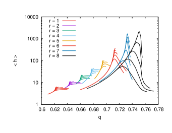
We verified that there is an abrupt change of the transition type at $r=r^{*}$, although we found $r^{*}$ somewhat closer to 7 than to 8, see Fig. 28. The most conspicuous feature in the range $1\leq r<r^{*}$ is a dramatic increase of the surface heights. For all $r$ the critical points are at those values of $q$ where $\langle h\rangle$ changes fastest, which is to the left of the peaks for $r<7$ and to its right for $r=8$. For all $r<7$ we found that the transition is not in the OP universality class, but in the universality class discussed in subsection III.B. This is most clearly seen for $r=1$, where simulations are fastest (due to the smallness of $\langle h\rangle$) and where also corrections to scaling are smallest. One might have anticipated that there are large scaling corrections for $r=1$ because of the nearness to $r=0$ where the model would be just ordinary site percolation, but this is not true. Indeed, we found critical exponents in perfect agreement with the estimates of subsection III.B, and with even somewhat smaller statistical errors. We do not show any plots as they are so similar to those in subsection III.B.

For $r>r^{*}$ the transitions look very much like first order transitions, in agreement with the claims in Li-Bashan ; Berezin2 ; Danziger . If so, then the transition should be tricritical exactly at $r^{*}$, but we were not able to measure tricritical exponents. As discussed in Li-Bashan ; Berezin2 ; Danziger , what happens at $r=r^{*}$ is that fronts become unstable. Consider a scenario where open sites exist only in half space $x>0$, while all sites with $x<0$ are closed. In ordinary percolation this would correspond just to a boundary where all clusters are cut off at $x<0$. This case of percolation in the presence of boundaries has been studied in detail Grass92 ; Cardy92 . In particular, the density of the giant cluster near the boundary is reduced and is governed by a new critical index, but otherwise the boundary has no effect on the bulk behavior.

This is still true for $r<r^{*}$, but not for $r>r^{*}$. Although we disagree with Li-Bashan ; Berezin2 ; Danziger on details and on the theoretical treatment, we agree with them that nodes near the boundary are removed from the viable cluster by dependencies, which leads then to more removals, etc., so that such boundaries create moving fronts which finally destroy the entire viable cluster – unless $q$ is large and $r$ is sufficiently close to $r^{*}$. If the front established in this latter case has a sharp profile and the density behind it is finite (which is clearly suggested by the simulations), one has a first order transition.

Figure 29: (color online) Densities of the largest viable cluster for the model of Li-Bashan with $r=12$, plotted against $q$ for various system sizes. Here, averages are taken over all runs, including those with no giant viable cluster.

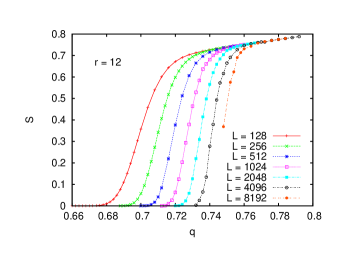
This gives thus indeed rise to the “upper” of the two claimed transitions for $r>r^{*}$ (where $q_{c}(r)>q_{c}(r^{*})\approx 0.74$) Li-Bashan ; Berezin2 ; Danziger – with an important caveat discussed below. But we found no indication for the lower transition, where $q_{c}$ is supposed to be lower than the critical value at $r^{*}$. In Fig. 29 we show the order parameter for $r=12$ (i.e., well above $r^{*}$) for system sizes between $L=128$ and $8192$. According to Li-Bashan ; Danziger , there should be a first order phase transition at $q=0.74$. We see that there is a rather rapid cross-over at $q=0.74$, if $L\approx 2000$ (which is presumably the size on which the claim of Li-Bashan ; Danziger was based), but we can definitely rule out a real phase transition within the range $0.68<q<0765$. Indeed, extrapolating to larger $L$ we can be rather sure that no transition occurs for any $q<0.8$. Notice that $q_{c}=0.753(1)$ for $r=8$ (data not shown), so the transition point is definitely increasing with increasing $r$. We cannot say numerically whether it agrees with the transition defined via the propagation of fronts (is at $q\approx 0.83$ for $r=12$), but this seems to be the only plausible option.

Analogous results were obtained for $r=20$ and $r=30$ (data not shown). Again we find rapid but nevertheless smooth crossovers at values of $q$ which increase rapidly with $L$. In both cases the cross-over happens at the “transition points” seen in Li-Bashan ; Danziger when $L\approx 10^{3}$, but we can rule out real phase transitions anywhere near these points.

Figure 30: (color online) Densities of the largest viable cluster for the model of Li-Bashan with $r=12$ (same data as in Fig. 28), but conditioned on clusters which do have a giant viable cluster.

Figure 31: (color online) Densities of giant viable clusters for $r=12,20,30$, and $\infty$.

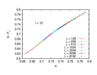
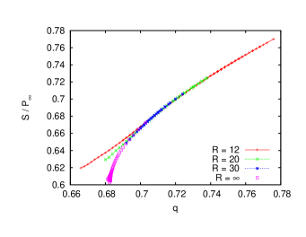
Further insight is obtained by plotting not the order parameter averaged over all runs, but by conditioning onto runs with a giant cluster. Again it is very easy to distinguish between runs with and without giant clusters (although the distinction is not as sharp as for $r=\infty$). The results for $r=12$ are plotted in Fig. 30. The perfect data collapse shows that the difference between the curves for different $L$ seen in Fig. 29 is entirely due to differences in the probabilities $P_{L}$ with which a giant cluster is reached. The structures of the giant clusters themselves are completely independent of $L$. In Fig. 31, these data are plotted together with analogous results for $r=20$ and $r=30$, and with the results for $r=\infty$ (obtained in the previous sub-subsection; see the inset in Fig. 26) extrapolated to $L\to\infty$. All four curves seem to become identical for large $q$, while they fan out systematically for small $q$. This figure suggests that there would be very little dependence on $r$ (except for very small $q$), if there were not a mechanism which would dramatically affect the probability for a giant viable cluster to occur.

Figure 32: (color online) Probabilities $1-P_{\infty}$ that no giant viable cluster is formed, for $r=12$.

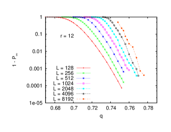
This mechanism is, as suggested in Li-Bashan ; Berezin2 ; Danziger , the existence of voids in the initial configuration and their subsequent growth. This is also confirmed by plotting the probabilities that a giant viable cluster is not formed, see Fig. 32 for $r=12$. For large $q$ (i.e., if these probabilities are small), they increase with $L$ as

$$1-P_{\infty}\sim c(q)L^{2},$$ (16)

suggesting that giant cluster formation is prevented by a rare extensive mechanism, i.e. by a mechanism whose probability to arise is $\propto L^{2}$. This is of course true for the formation of voids in the initial configuration. We also see that these probabilities decrease, for fixed $L$, roughly exponentially with $q$. This is again what we would expect for the random formation of voids, with

$$p(m)\sim\frac{L^{2}}{m}(1-q)^{m}$$ (17)

being roughly the probability to form a void of $m$ sites. Numerical estimates of void sizes based on this estimate and on Fig. 32 give void sizes which are typically half as large as those quotes in Li-Bashan . This is not unreasonable, given the fact that voids were assumed in Li-Bashan to be circular disks, while they could indeed have different shapes.

Thus we do agree with basic features proposed in Li-Bashan ; Berezin2 ; Danziger , but we do not agree with the existence of a second phase transition curve. We also would not call “metastable” the states for $q$ slightly above this supposed transition curve, since metastability applies to systems subject to stochastic (not frozen) noise, and refers to states which are actually unstable on long time scales. In the present case we would rather speak of “conditional stability”, since the viable clusters are absolutely stable, but they arise only conditioned on particular initial configurations.

III.6.4 A Final Remark on First Order Transitions and an Alternative Scenario

As we said, the data suggest for $r>r^{*}$ a first order transition, and the location of this transition seems to be on the curve given in Li-Bashan ; Berezin2 ; Danziger . Although we have no direct numerical evidence to doubt this, there is indirect evidence and theoretical arguments. As suggested in Li-Bashan ; Berezin2 ; Danziger , the transition for $r>r^{*}$ is essentially a percolation transition, where the spreading of voids induced by dependencies becomes critical. In $d\geq 3$ there exist indeed tricritical points in generalized percolation models where the phase transition changes from second to first order Janssen ; Bizhani2 . There is however strong evidence Bizhani2 ; Dahmen ; Bizhani3 that such tricritical points are absent in $d=2$. This seems related to the Aizenman-Wehr theorem Aizenman2 on absence of first order phase transitions in random 2-d systems, although details are far from clear. Physically, it corresponds to the fact that phase boundaries cannot stay flat in 1+1 - dimensional isotropic random systems, but become crumpled on large scales. This is e.g. what is found in the $T=0$ random field Ising model Dahmen ; Bizhani3 , and such interfaces seem always to be in the OP universality class, even if they look very smooth on small scales Note3 .

Figure 33: (color online) Densities of giant viable clusters on 2-d lattices of size $L_{\perp}\times L_{\|}=2048\times 16384$, with $r=9$ and $q=0.772$ (which is our best estimate for $q_{c}$ at $r=9$). Shown are the 1-d projections of these densities for ten typical realizations, multiplied with arbitrary factors to avoid overlaps. Due to local isotropy, we would expect that interface widths should become $\sim L_{\perp}$ in the large system limit. Actual interfaces are much sharper.

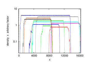
As suggested by Fig. 33, this is not true for simulations on lattices of size $L_{\perp}\times L_{\|}$ with $L_{\|}\gg L_{\perp}$, and with zero initial densities in the regions $x<x_{-}=20$ and $x>x_{+}=L_{\|}-20$. The latter enforce interfaces which would stay near $x_{\pm}$ if $q>q_{c}$, but move inwards for $q<q_{c}$. We find, even for $r$ very close to $r^{*}$, that interfaces at $q\approx q_{c}$ are very straight, with fluctuations much smaller than $L_{\perp}$. For larger values of $r$ (data not shown) the effect was much enhanced, and the interfaces were essentially straight lines. This is clearly a finite size effect, which is particularly enhanced by the specific choice of dependency links made in Li-Bashan ; Berezin2 ; Danziger : By choosing such links to be in a square region with sharp boundaries, fluctuations of the interface are strongly suppressed.

We thus conclude that all simulations of Li-Bashan ; Berezin2 ; Danziger are far from the true asymptotic region. It might be that the positions of the critical points are nevertheless correct, but they may also be far off. In any case, the fact that the transitions for $r>r^{*}$ look like first order cannot be taken as evidence that they really are so. Explosive percolation Achlioptas should be a warning that not all transitions that look first order also are so. In the present case, the length scale introduced by $r$ should be enough to confuse the picture.

Indeed, we conjecture that the transition is in the universality class of OP not for $r<r^{*}$ (as claimed in Li-Bashan ), but for $r>r^{*}$ – where it just corresponds to ordinary percolation of voids. We have to admit that we do not have direct numerical evidence to support this claim, nor do we see any possibility to obtain evidence in favor or against it in the near future.

IV Discussion

The purpose of this paper was twofold: On the one hand, we proposed an efficient algorithm to simulate viable clusters in multiplex networks, and the percolation transitions related to them. This was motivated by the fact that exact results for this problem are obtainable only in mean field theory (i.e. on random locally loopless graphs), and there exist ample indications that such predictions can be very misleading in real applications. Indeed, the algorithm presented in this paper is not only fast, but by mapping the problem onto a solid-on-solid model we were able also to discuss some non-trivial structures which might become important for themselves.

The other aim of the paper was to apply this algorithm in several simple networks and lattices, in order to test previous claims and to understand better the nature of the percolation transition(s) in this model. We found several surprises:

• While the geometric structure of viable clusters on ER networks is indeed as predicted by mean field theory, it seems that the (pseudo-)dynamics of cascades is not. We speculated that this might be because the clusters are supercritical during the cascades, but more work is needed to understand this.

• On finite-dimensional lattices the model is not in the universality class of ordinary percolation, but represents its own new universality class. This is seen most dramatically in four and five dimensions, where OP would show continuous transitions with non-trivial anomalous exponents. Rather, we found a first order transition in $d=5$, and a continuous transition with $\beta=1$ in $d=4$. Thus it seems as if the model has upper critical dimension $d_{u}=4$, although the true mean field solution has a discontinuous transition. In $d=2$ the results are less dramatic, but it seems clear that it is not in the OP universality class. In $d=3$, finally, we cannot make a clear statement because of very strong corrections to scaling.

• While the order parameter exponent is $\beta=1$ for $d=4$ as in other models at the upper critical dimension, other exponents like the fractal cluster dimension and the correlation length are different. They seem to be simple rational numbers, but precise estimates are difficult due to strong (logarithmic?) corrections.

• In general, all first order transitions are hybrid. Thus, the order parameter makes on ER networks and on 5-dimensional lattices not only a jump, but it also shows a power law. More surprisingly, in $d=5$ there seems also to be a non-trivial scaling mass distribution of finite clusters.

As regards geometric networks embedded in low dimensions with semi-local links, we partly confirmed the scenario found in Li-Bashan . We do not find the double phase transitions claimed there when the lengths of these links are are above a (tri-)critical value. We do find that there exists such a (tri-)critical value above which the transition seems to be first order, but we give strong evidence that this is related to very large finite size corrections. More importantly, we claim that the model studied in Li-Bashan ; Berezin2 ; Danziger is very unrealistic in assuming dependency links to be much longer than connectivity links. Whether a model where this relation is reversed shows similar behavior is an open question.

Other open questions concern the behavior of multiplex networks with $>2$ types of links. We have not yet tried to extend our algorithm to this case. Even less clear is the behavior in case of non-mutual (asymmetric) dependencies, which cannot be mapped onto multiplex networks at all. The same is true for directed multiplex networks. Finally, the true asymptotic behavior in the 2-d case with long range dependency links could, eventually, only be solved analytically or by means of a different model realization which avoids the introduction of a new length scale.

References

- (1) N.A.M. Araújo, P. Grassberger, B. Kahng, K.J. Schrenk, and R.M. Ziff, European Phys. J. 223, 2307 (2014).
- (2) D.S. Callaway, J.E. Hopcroft, J.M. Kleinberg, M.E.J. Newman, and S.H. Strogatz, Phys. Rev. E 64, 041902 (2001).
- (3) S. Boettcher, V. Singh, and R.M. Ziff, Nature Commun. 3, 787 (2012).
- (4) G. Bizhani, P. Grassberger, and M. Paczuski, Phys. Rev. E 84, 066111 (2011).
- (5) H.W. Lau, M. Paczuski, and P. Grassberger, Phys. Rev. E 86, 011118 (2012).
- (6) D. Achlioptas, R.M. D’Souza, and J. Spencer, Science 323, 1454 (2009).
- (7) S.V. Buldyrev, R. Parshani, G. Paul, H.E. Stanley, and S. Havlin, Nature 464, 1065, (2010).
- (8) P.S. Dodds and D.J. Watts, Phys. Rev. Lett. 92, 218701 (2004).
- (9) H.K. Janssen, M. Müller, and O. Stenull, Phys. Rev. E 70, 026114 (2004).
- (10) G. Bizhani, M. Paczuski, and P. Grassberger, Phys. Rev. E 86, 011128 (2012).
- (11) L. Chen, F. Ghanbarnejad, W. Cai, and P. Grassberger, Europhys. Lett. 104, 50001 (2013).
- (12) W. Cai, F. Ghanbarnejad, L. Chen, and P. Grassberger, to be published (2014).
- (13) M. Aizenman and C.M. Newman, Commun. Math. Phys. 107, 611 (1986).
- (14) P. Grassberger, J. Stat. Mech. P04004 (2013).
- (15) J. Chalupa, P.L. Leath, and G.R. Reich, J. Phys. C: Solid State Phys. 12 L31 (1979).
- (16) J. Adler, Physica A 171, 453 (1991).
- (17) A. V. Goltsev, S. N. Dorogovtsev, and J. F. F. Mendes, Phys. Rev. E 73, 056101 (2006).
- (18) A forerunner of bootstrap percolation was the threshold model of Granovetter Granovetter .
- (19) G.J. Baxter, S.N. Dorogovtsev, A.V. Goltsev, J.F.F. Mendes, Phys. Rev. E 83, 051134 (2011).
- (20) P. Grassberger, C. Christensen, G. Bizhani, S.-W. Son, and M. Paczuski, Phys. Rev. Lett. 106, 225701 (2011).
- (21) M. E. J. Newman, S.H. Strogatz, and D.J. Watts, Phys. Rev. E 64, 026118 (2001).
- (22) M. E. J. Newman, Phys. Rev. E 66, 016128 (2002).
- (23) B. Bollobás, Random Graphs (Springer, New York 1998).
- (24) S.-W. Son, G. Bizhani, C. Christensen, P. Grassberger, and M. Paczuski, Europhys. Lett. 97, 16006 (2012).
- (25) R. Parshani, S.V. Buldyrev, and S. Havlin, Phys. Rev. Lett. 105, 048701 (2010).
- (26) J. Gao, S.V. Buldyrev, H.E. Stanley, and S. Havlin, Nature Physics 8, 40 (2012).
- (27) S.-W. Son, P. Grassberger, and M. Paczuski, Phys. Rev. Lett. 107, 195702 (2011).
- (28) B. Karrer and M.E.J. Newman, Phys. Rev. E 82, 016101 (2010).
- (29) B. Karrer, M.E.J. Newman, and L. Zdeborová, e-print arXiv 1405.0483 (2014).
- (30) M. Shrestha and C. Moore, e-print arXiv:1312.2070 (2013).
- (31) Y. Shiraki and Y. Kabashima, Phys. Rev. E 82, 036101 (2010).
- (32) S. Watanabe and Y. Kabashima, e-print arXIV:1308.1210 (2013).
- (33) A. Bashan and S. Havlin, J. Stat. Phys. 145, 686 (2011).
- (34) A. Bashan, R. Parshani, and S. Havlin, Phys. Rev. E 83, 051127 (2011).
- (35) W. Li, A. Bashan, S.V. Buldyrev, H.E. Stanley, and S. Havlin, Phys. Rev. Lett. 108, 228702 (2012).
- (36) A. Bashan, Y. Berezin, S.V. Buldyrev, and S. Havlin, Nature Physics 9, 667 (2013).
- (37) Y. Berezin, A. Bashan, M.M. Danziger, D. Li, and S. Havlin, e-print arXiv:1310.0996 (2013).
- (38) G.J. Baxter, S.N. Dorogovtsev, A.V. Goltsev, J.F.F. Mendes, Phys. Rev. Lett. 109, 248701 (2012).
- (39) L.D. Valdez, P.A. Macri, H.E. Stanley, and L.A. Braunstein, Phys. Rev. E 88, 050803 (2013).
- (40) D. Cellai, E. López, J. Zhou, J.P. Gleeson, and G. Bianconi, e-print arXiv:1307.6359 (2013).
- (41) M. Stippinger and J. Kertész, e-print arXiv:1312.1993 (2013).
- (42) M.M. Danziger, A. Bashan, Y. Berezin, and S. Havlin, J. Complex Networks, to be published (2014).
- (43) D. Zhou, A. Bashan, R. Cohen, Y. Berezin, N. Shnerb, and S. Havlin, arXiv:1211.2330v3 (2014).
- (44) S. Hwang, S. Choi, Deokjae Lee, and B. Kahng, e-print arXiv:1409.1147 (2014).
- (45) There exists also a fast algorithm to find the largest viable cluster Schneider , but since only the largest cluster is followed during the cascade, it might give wrong results in cases where an initially large cluster is taken over during the cascade by a cluster that had started smaller. This does not happen on random tree-like graphs, but it might happen on more general graphs.
- (46) V. Privman and N. vrakić, J. Stat. Phys. 51, 1111 (1988).
- (47) P.L. Leath, Phys. Rev. B 14, 5046 (1976).
- (48) B. Min and K.-I. Goh, e-print arXiv:1401.1587 (2014).
- (49) Notice that our families of waves are similar but yet different from the “cascades” discussed in Buldyrev . The latter are nested sequences of clusters which all contain the maximal viable cluster, while in our algorithm the nested clusters all contain the same seed .
- (50) D. Dhar, Phys. Rev. Lett. 64, 1613 (1990).
- (51) Y. Berezin, A. Bashan, and S. Havlin, Phys. Rev. Lett. 111, 189601 (2013).
- (52) S.W. Son, P. Grassberger, and M. Paczuski, Phys. Rev. Lett. 111, 189602 (2013).
- (53) C.D. Lorenz and R.M. Ziff, Phys. Rev. E 57, 230 (1998).
- (54) Y.J. Deng and H.W.J. Blote, Phys. Rev. E 72, 016126 (2005).
- (55) P. Grassberger, J. Stat. Phys. 153, 289 (2013).
- (56) P. Grassberger, J. Phys. A: Mathematical and General 25, 5867 (1992).
- (57) J.L. Cardy, J. Phys. A: Mathematical and General 25, L201 (1992).
- (58) B. Drossel and K. Dahmen, European Phys. J. 3, 485 (1998).
- (59) G. Bizhani, M. Paczuski, and P. Grassberger, to be published.
- (60) M. Aizenman and J. Wehr, Phys. Rev. Lett. 62, 2503 (1989).
- (61) Notice that interfaces in 1+1-dimensional systems are smooth, as long as they are not pinned but moving, as in the KPZ problem or Eden growth.
- (62) M. Granovetter, Am. J. Sociol. 83, 1420 (1978).
- (63) C.M. Schneider, N.A.M. Araújo, and H.J. Herrmann, Phys. Rev. E 87, 043302 (2013).
- (64) Because sites are indexed for helical b.c. by single indices, this leads to slightly simpler and faster codes. For the sizes used in this paper, periodic and helical b.c. lead to numerically indistinguishable results.