28
Planck 2015 results. XVII. Constraints on primordial non-Gaussianity
The Planck full mission cosmic microwave background (CMB) temperature and -mode polarization maps are analysed to obtain constraints on primordial non-Gaussianity (NG). Using three classes of optimal bispectrum estimators — separable template-fitting (KSW), binned, and modal — we obtain consistent values for the primordial local, equilateral, and orthogonal bispectrum amplitudes, quoting as our final result from temperature alone , , and (68 % CL, statistical). Combining temperature and polarization data we obtain , , and (68 % CL, statistical). The results are based on comprehensive cross-validation of these estimators on Gaussian and non-Gaussian simulations, are stable across component separation techniques, pass an extensive suite of tests, and are consistent with estimators based on measuring the Minkowski functionals of the CMB. The effect of time-domain de-glitching systematics on the bispectrum is negligible. In spite of these test outcomes we conservatively label the results including polarization data as preliminary, owing to a known mismatch of the noise model in simulations and the data. Beyond estimates of individual shape amplitudes, we present model-independent, three-dimensional reconstructions of the Planck CMB bispectrum and derive constraints on early universe scenarios that generate primordial NG, including general single-field models of inflation, axion inflation, initial state modifications, models producing parity-violating tensor bispectra, and directionally dependent vector models. We present a wide survey of scale-dependent feature and resonance models, accounting for the “look elsewhere” effect in estimating the statistical significance of features. We also look for isocurvature NG, and find no signal, but we obtain constraints that improve significantly with the inclusion of polarization. The primordial trispectrum amplitude in the local model is constrained to be (68 % CL statistical), and we perform an analysis of trispectrum shapes beyond the local case. The global picture that emerges is one of consistency with the premises of the CDM cosmology, namely that the structure we observe today was sourced by adiabatic, passive, Gaussian, and primordial seed perturbations.
Key Words.:
cosmology: cosmic background radiation – cosmology: observations – cosmology: theory – cosmology: early Universe – cosmology: inflation – methods: data analysis1 Introduction
This paper, one of a set associated with the 2015 release of data from the Planck111Planck (http://www.esa.int/Planck) is a project of the European Space Agency (ESA) with instruments provided by two scientific consortia funded by ESA member states and led by Principal Investigators from France and Italy, telescope reflectors provided through a collaboration between ESA and a scientific consortium led and funded by Denmark, and additional contributions from NASA (USA). mission (Planck Collaboration I 2016), describes the constraints on primordial non-Gaussianity (NG) obtained using the cosmic microwave background (CMB) maps from the full Planck mission, including a first analysis of some of the Planck polarization data.
Primordial NG is one of the most powerful tests of inflation, and more generally of high-energy early Universe physics (for some reviews, see Bartolo et al. 2004a, Liguori et al. 2010, Chen 2010b, Komatsu 2010, Yadav & Wandelt 2010). In fact, the simplest models of inflation (characterized by a single scalar field slowly rolling along a smooth potential) predict the generation of primordial fluctuations that are almost Gaussian distributed, with a tiny deviation from Gaussianity of the order of the slow-roll parameters (Acquaviva et al. 2003; Maldacena 2003). The 2013 Planck results on primordial NG are consistent with such a prediction, being compatible with Gaussian primordial fluctuations: the standard scenario of single-field, slow-roll inflation has survived its most stringent test to date. For example, in Planck Collaboration XXIV (2014) we obtained , , and for the amplitudes of three of the most well-studied shapes of primordial NG. On the other hand, it is well known that any deviations from the standard picture of inflation have the potential to produce distinctive NG signatures at a detectable level in the CMB anisotropies.222We refer the reader to Planck Collaboration XXIV (2014) and references therein for a detailed summary of the models and underlying physical mechanisms generating various types of primordial NG. Therefore, as already shown in Planck Collaboration XXIV (2014) (see also Planck Collaboration XXII (2014)) improved NG constraints allow severe limits to be placed on various classes of inflationary models that extend the simplest paradigm, in a way that is strongly complementary to the power-spectrum constraints (i.e., scalar spectral index of curvature perturbations and tensor-to-scalar amplitude ratio).
One of the main goals of this paper is to improve NG constraints using mainly the angular bispectrum of CMB anisotropies, i.e., the harmonic transform of the 3-point angular correlation function. We also investigate higher-order NG correlators like the trispectrum. We follow the same notation as Planck Collaboration XXIV (2014). The CMB angular bispectrum is related to the primordial bispectrum
| (1) |
where the field , related to the comoving curvature perturbation on super-horizon scales by , is such that in the matter era, and on super-horizon scales, it reduces to Bardeen’s gauge-invariant gravitational potential (Bardeen 1980). The bispectrum measures the correlation among three perturbation modes. If translational and rotational invariance are assumed, it depends only on the magnitude of the three wavevectors. In general the bispectrum can be written as
| (2) |
where we have introduced the dimensionless “nonlinearity parameter” (Gangui et al. 1994; Wang & Kamionkowski 2000; Komatsu & Spergel 2001; Babich et al. 2004), measuring the NG amplitude. The bispectrum is obtained by sampling triangles in Fourier space. The dependence of the function on the type of triangle (i.e., the configuration) formed by the three wavevectors describes the shape (and the scale dependence) of the bispectrum (Babich et al. 2004), which encodes much physical information. Different NG shapes are linked to distinctive physical mechanisms that can generate such NG fingerprints in the early Universe.
In this paper the limits on primordial NG are mainly improved through the use of the full mission data, as well as by exploiting the polarization information.
Planck results on primordial NG also provide a reconstruction of the full CMB bispectrum through different techniques (see Sect. 6.2). This complements (and adds to) the extraction of single amplitudes for specific bispectrum shapes. Such a reconstruction can point to interesting features in the bispectrum signal that go beyond the usual standard scale-invariant shapes (such as the well known “local” and “equilateral” configurations).
As we have seen, the Planck 2013 NG paper (Planck Collaboration XXIV 2014) significantly improved constraints on the standard primordial NG models with scale-invariant local, equilateral or orthogonal shapes. The Planck NG paper also included constraints from the modal estimator on a variety of other primordial models, including DBI inflation, non-Bunch-Davies models (excited initial states), directionally-dependent vector inflation models, warm inflation, and scale-dependent feature and resonance models. All scale-invariant bispectra were strongly constrained, with the possible exception of highly flattened non-Bunch-Davies models. On the other hand, the preliminary investigation of primordial oscillatory models seemed to be more promising, in that two specific feature models appeared to produce fits of some significance. One aim of the present work is to expand the detail and scope of investigations of feature and resonant models and to examine the significance of these results with a more careful analysis of the “look elsewhere” effect, through exploring multi-parameter results using large ensembles of Gaussian simulations. Also we will thoroughly analyse or re-analyse other primordial NG signals that are theoretically well-motivated and those which have appeared in the literature since the first data release. These include primordial NG arising in the context of inflation models where vector fields play a non-negligible role or primordial NG generated in the tensor (gravitational waves) perturbations. Each of these primordial NG signals carry distinctive signatures that may have been imprinted at the inflationary epoch, thus opening up a new window into the detailed physics of inflation.
The paper is organized as follows. In Sect. 2 we briefly discuss the primordial NG models that we test in this paper. Section 3 summarizes the optimal statistical estimators used to constrain the CMB bispectrum and trispectrum from Planck temperature and polarization data. In Sect. 4 we discuss the non-primordial contributions to the CMB bispectrum and trispectrum, including foreground residuals after component separation and focusing on the bias induced by the ISW-lensing bispectrum. We also analyse the impact on primordial NG estimation from the residuals of the deglitching processing. Section 5 describes an extensive suite of tests performed on realistic simulations to validate the different estimator pipelines, and compare their performance. Using simulations, we also quantify the impact on of using a variety of component-separation techniques. In Sect. 6 we derive constraints on for the local, equilateral, and orthogonal bispectra and present a reconstruction of the CMB bispectrum. We also present a reconstruction of the primordial curvature fluctuations. In Sect. 7 we validate these results by performing a series of null tests on the data to assess the robustness of our results. Section 8 investigates scale-dependent NG models and other selected bispectrum shapes. Section 9 presents the Planck limits on the CMB trispectrum. In Sect. 10 we provide constraints on CMB local bispectrum and trispectrum from Minkowski functionals. In Sect. 11 we discuss the main implications of Planck’s constraints on primordial NG for early Universe models. We conclude in Sect. 12. Appendix A contains the derivation of the statistical estimator for the amplitudes characterizing a “direction-dependent” primordial non-Gaussianity. Appendix B contains some details about Minkowski functionals.
2 Models
In this Section we briefly highlight the classes of inflationary models investigated in this paper, and describe the distinctive NG they generate. Within each class a common underlying physical process gives rise to the corresponding NG shape, illustrated by concrete realizations of inflationary models. For each class we therefore provide the explicit form of the bispectrum shapes chosen for the data analysis, emphasizing extensions with variants and distinctly new shapes beyond those already described in Planck Collaboration XXIV (2014).
2.1 General single-field models of inflation
This class of models includes inflationary models with a non-standard kinetic term (or more general higher-derivative interactions), in which the inflaton fluctuations propagate with an effective sound speed which can be smaller than the speed of light. For example, models with a non-standard kinetic term are described by an inflaton Lagrangian , where , with at most one derivative on , and the sound speed is given by .
The NG parameter space of this class of models is generically well described by two NG shapes — “equilateral” and “orthogonal” (Senatore et al. 2010) — since usually there are two dominant interaction terms of the inflaton field giving rise to the overall NG signal. One of these typically produces a bispectrum very close to the equilateral type with in the limit (Chen et al. 2007b; Senatore et al. 2010).
The equilateral-type NG is well approximated by the template (Creminelli et al. 2006)
| (3) | |||||
Here represents Bardeen’s gravitational potential power spectrum, being the normalization and the scalar spectral index. DBI inflationary models based on string theory (Silverstein & Tong 2004; Alishahiha et al. 2004) provide physically well-motivated examples of the -model. They are characterized by an almost equilateral NG with for , which typically is .
The “orthogonal” shape template is (Senatore et al. 2010)
| (4) | |||||
Equilateral and orthogonal shapes emerge also in models characterized by more general higher-derivative interactions, such as ghost inflation (Arkani-Hamed et al. 2004), effective field theories of inflation (Cheung et al. 2008; Senatore et al. 2010; Bartolo et al. 2010a), or the so “Galileon-like” models of inflation (see, e.g., Burrage et al. 2011). The latter model is constructed starting from some specific underlying symmetry for the inflaton field, and is characterized by strongly constrained derivative interactions.
2.2 Multi-field models
This class of models is characterized by the presence of additional light scalar degrees of freedom besides the inflaton, whose fluctuations give rise, or contribute, to the final primordial curvature perturbation at the end of inflation. This includes the case of “multiple-field inflation”, where inflation is driven by more than one scalar field, as well as scenarios in which additional scalar fields remain subdominant during the inflationary expansion. From the point of view of primordial NG, the element in common to all these models is that a potentially detectable level of NG in the curvature perturbation is generated via a transfer of super-horizon non-Gaussian isocurvature perturbations in the second field (not necessarily the inflaton) to the adiabatic (curvature) density perturbations, accompanied by nonlinearities in the transfer mechanism. This process typically takes place on super-horizon scales, thus implying a local form of NG in real space. When going to Fourier space, this leads to a correlation between large and small scale modes. The bispectrum for this class of models is indeed largest on so-called “squeezed” triangles (). The local bispectrum is (Falk et al. 1993; Gangui et al. 1994; Gangui & Martin 2000; Verde et al. 2000; Wang & Kamionkowski 2000; Komatsu & Spergel 2001)
| (5) | |||||
There is a broad literature on examples and specific realizations of this transfer mechanism from isocurvature to adiabatic perturbations (Bartolo et al. 2002; Bernardeau & Uzan 2002; Vernizzi & Wands 2006; Rigopoulos et al. 2006, 2007; Lyth & Rodriguez 2005; Tzavara & van Tent 2011; for a review on NG from multiple-field inflation models, see Byrnes & Choi 2010). An alternative, important possibility is the curvaton model (Mollerach 1990; Linde & Mukhanov 1997; Enqvist & Sloth 2002; Lyth & Wands 2002; Moroi & Takahashi 2001). In this type of scenario, a second light scalar field, subdominant during inflation, decays after inflation, generating primordial density perturbations with a potentially high level of NG (e.g., Lyth & Wands 2002; Lyth et al. 2003; Bartolo et al. 2004c). In the (simplest) adiabatic curvaton models, the local parameter was found to be (Bartolo et al. 2004c, b) , when the curvaton field has a quadratic potential (Lyth & Wands 2002; Lyth et al. 2003; Lyth & Rodriguez 2005; Malik & Lyth 2006; Sasaki et al. 2006). In the previous formula, is the “curvaton decay fraction” evaluated at the epoch of the curvaton decay in the sudden decay approximation. It is then easy to see that, for low values of , a high level of NG can be generated. 333NG perturbations can arise also at the end of inflation, e.g., from nonlinearities during the (p)reheating phase (e.g., Enqvist et al. 2005; Chambers & Rajantie 2008; Barnaby & Cline 2006; see also Bond et al. 2009) or from fluctuations in the inflaton decay rate or interactions, as found in modulated (p)reheating and modulated hybrid inflation (Kofman 2003; Dvali et al. 2004a, b; Bernardeau et al. 2004; Zaldarriaga 2004; Lyth 2005; Salem 2005; Lyth & Riotto 2006; Kolb et al. 2006; Cicoli et al. 2012).
2.3 Isocurvature non-Gaussianity
Isocurvature NG, which was only sketched from the purely theoretical point of view in the 2013 paper, can now be analysed thanks to the polarization information.
In most of the models mentioned above, the main focus is on the level of primordial NG in the final curvature perturbation . However, in inflationary scenarios where different scalar fields play a non-negligible role, residual isocurvature perturbation modes can remain after inflation. Isocurvature modes are usually investigated by considering their contribution to the power spectrum. However, if present, they would also contribute to the bispectrum, producing in general both a pure isocurvature bispectrum and mixed bispectra because of the cross-correlation between isocurvature and adiabatic perturbations (Komatsu 2002; Bartolo et al. 2002; Komatsu et al. 2005; Kawasaki et al. 2008; Langlois et al. 2008; Kawasaki et al. 2009; Hikage et al. 2009; Langlois & Lepidi 2011; Langlois & van Tent 2011; Kawakami et al. 2012; Langlois & van Tent 2012). While one might expect isocurvature NG to be negligible, since both (linear) isocurvature modes and (adiabatic) NG appear to be very small, and searches for isocurvature NG using WMAP data did not lead to any detections (Hikage et al. 2013a, b), this expectation can be tested at significantly higher precision by Planck. Moreover, there exist inflation models (Langlois & Lepidi 2011) where isocurvature modes, while remaining a small fraction in the power spectrum, would dominate the bispectrum.
At the time of recombination there are in principle four possible distinct isocurvature modes (in addition to the adiabatic mode): cold dark matter (CDM); baryon; neutrino density; and neutrino velocity isocurvature modes (Bucher et al. 2000). In this paper we will only consider isocurvature NG of the local type and always limit ourselves to considering the adiabatic mode together with just one type of isocurvature mode (considering each of the four types separately). Otherwise the number of free parameters becomes so large that no meaningful limits can be derived. Moreover, we assume the same spectral index for the primordial isocurvature power spectrum and the isocurvature-adiabatic cross-power spectrum as for the adiabatic power spectrum. Under those assumptions, as shown by Langlois & van Tent (2011), we have in principle six independent parameters: the usual purely adiabatic one; a purely isocurvature one; and four correlated ones.
The primordial shape templates are a generalization of Eq. (5), see Langlois & van Tent (2011, 2012):
| (6) | |||||
where label the different modes (adiabatic and isocurvature). The invariance under the simultaneous exchange of two of these indices and the corresponding momenta means that , hence reducing the number of independent parameters from eight to six, in the case of two modes. The different bispectra vary most importantly through the fact that different types of radiation transfer functions are used to project the primordial template onto the CMB: the reduced bispectra are of the form
| (7) |
with
| (8) | |||||
| (9) |
Here is the spherical bessel function and we use the notation . In addition to the isocurvature index, each transfer function carries a polarization index that we do not show here. It is important to note that, unlike the case of the purely adiabatic mode, the inclusion of polarization improves the constraints on the isocurvature NG significantly, as predicted by Langlois & van Tent (2011, 2012).
2.4 Resonance and axion monodromy models
Oscillatory models for NG are physically well-motivated. Large-field inflation faces an inherent UV completion problem because the inflaton field is required to move over large distances in field space relative to the Planck mass . An effective shift symmetry can enforce potential flatness and this can be naturally implemented in a string theory context with axions and a periodically modulated potential, so-called “axion monodromy” models. This periodicity can generate resonances in the inflationary fluctuations with logarithmically-spaced oscillations, creating imprints in the power spectrum, the bispectrum and trispectrum (Chen et al. 2008; Flauger et al. 2010; Hannestad et al. 2010; Flauger & Pajer 2011). On the other hand, sharp features or corners in an inflationary potential can temporarily drive the inflaton away from slow-roll; these large changes in the field and derivatives can create evenly-spaced oscillations, to be discussed in the next subsection. However, in multifield models residual oscillations after corner-turning can also lead to log-spaced oscillations, just as in the resonance models (Chen 2011; Achúcarro et al. 2011; Battefeld et al. 2013; Chen et al. 2015). A preliminary search for bispectrum resonance signals was performed in the first Planck analysis (Planck Collaboration XXIV 2014) and our purpose here is to substantially increase the frequency range and number of models investigated.
Simple resonance model: Periodic features in the inflationary potential can induce oscillations with frequency that can resonate through any interactions with the inflationary fluctuations, contributing to the bispectrum. Provided that , this mode starts inside the horizon but its frequency decreases as it is stretched by inflation, until frozen when . Thus periodic features introduce a driving force which can scan across a wide range of frequencies. The simplest basic behaviour of such resonant models yields logarithmic stretching and can be described by the non-scale-invariant shape (see Chen et al. 2008; Chen 2010b)
| (10) |
where the constant , is a wavenumber associated with the periodicity, and is a phase. These oscillations constructively and destructively interfere with the oscillations created by the CMB transfer functions, introducing additional nodal points in the CMB bispectrum.
Generalized resonance models: In a more general context, it is possible to have more complicated resonant shapes and envelopes. Resonant single-field models with varying sound speed generate three leading-order bispectrum terms (Chen 2010a):
| (11) |
The first term on the right-hand side of Eq. (2.4) is the basic resonant shape given in Eq. (10), while the second and third terms have the same oscillatory behaviour, but modulated by a (mildly) flattened shape, and an equilateral shape respectively. The third term is in fact the second generic shape arising in effective field theory and correlates well with the equilateral shape in Eq. (12). The second term in Eq. (2.4) weakly favours flattened triangles, but there are regimes for resonant models that can generate much stronger flat shapes. If the resonance begins very deep inside the horizon, then the second (negative energy) mode can also make a significant contribution that is associated with enfolded or flat bispectra; this is similar to having an excited initial state or non-Bunch-Davies (NBD) vacuum.
With these two physical motivations in mind we also investigate classes of models with resonant oscillations modulated by both the equilateral and flattened shapes, defined by
| (12) |
where (here, for simplicity we ignore the spectral index dependence of the equilateral shape in Eq. 3). The corresponding equilateral and flattened resonant bispectra ansätze are then
| (13) | |||
| (14) |
We note that typically non-Bunch-Davies bispectra can be much more sharply peaked in the flattened or squeezed limits than Eq. (14), but our purpose here is to determine if this type of resonant model is favoured by the Planck data; that is, whether Eq. (14) warrants further investigation with other flattened profiles.
2.5 Scale-dependent oscillatory feature models
Temporary violations of slow-roll inflation can occur if there are sharp features in the inflationary potential (Chen et al. 2007a), as well as changes in the sound speed or sharp turns in field space in multifield inflation. The inflaton field makes temporary departures from the attractor solution, which typically have a strong scale-dependent running modulated by a sinusoidal oscillation; there are model-dependent counterparts in the power spectrum, bispectrum, and trispectrum. For example, sharper or narrower features induce a relatively larger signal in the bispectrum (see e.g., Chen 2010b). An example is the analytic envelope solutions predicted for both the power spectrum and bispectrum for the single field models with a specific inflaton feature shape (Adshead et al. 2012); a search for these was presented previously in the Planck Inflation paper (Planck Collaboration XXII 2014) and likewise no significant signal was found using the corresponding bispectrum envelopes at the available modal resolution (Planck Collaboration XXIV 2014). In this new analysis, we will emphasize the search for generic oscillatory behaviour in the data over a larger range in modal resolution, although we will also look for the shapes predicted for simple features in single field models.
Constant feature model: In the previous investigation of Planck data using a coarse parameter grid (Planck Collaboration XXIV 2014), we searched for the simplest ansatz for an oscillatory bispectrum signal (Chen et al. 2007a):
| (15) |
where is a phase factor and is a frequency associated with the specific shape of the feature in the potential that disrupts the slow-roll evolution. In the earlier analysis, we also considered a damping envelope, which slightly increased the apparent significance of the best-fit feature models, though at the cost of an additional parameter (see single-field solutions below).
Generalized feature models: Here, we again search for oscillatory signals in a model-independent manner. We will modulate the bispectrum cross-sections with the physically motivated equilateral and flattened shapes, reflecting the physical contexts in which they could have been generated, as for the resonant models described above in Eq. (2.4). If there are potential features in a model with a varying sound speed, then we can expect there to be oscillatory contributions to the bispectrum signal with a dominant equilateral shape. Motivated by the equilateral resonance model in Eq. (2.4), we will search for the following equilateral feature ansatz:
| (16) | |||
| (17) |
For extremely sharp features, it is possible to excite the inflationary fluctuations as if there were a non-Bunch Davies vacuum: the oscillatory signal becomes modulated with a flattened shape (Chen et al. 2007a). Again, motivated by the enfolded resonance model in Eq. (14), we take the following simple flattened ansatz:
| (18) |
Although the exact profile of the flattened shape can be much more highly peaked on the faces in these NBD models, this ansatz should be adequate for testing whether these models are favoured. We note that while the power spectrum is insensitive to the underlying scenario creating the features, the bispectrum shape will reveal whether features arise from varying sound speed or highly excited features in the potential.
Single field feature solutions: Here we use the full analytic bispectrum solution given by Adshead et al. (2012), but the dominant leading-order behaviour takes the form
| (19) |
where and is an envelope function, with parameter setting an overall cut-off for the bispectrum at large wavenumbers or multipoles. This envelope and the overall scaling distinguishes this realistic case from the simple separable constant feature ansatz of Eq. (15). We shall allow the envelope parameter to vary from , with no envelope (the infinitely thin limit for a feature in the potential) through to large , with a narrow domain for the bispectrum. Alternative analytic solutions where the bispectrum is created by a variation in the sound speed are dominated by the term, as in
| (20) |
For the simplest models there is a predicted relationship between the power spectrum and bispectrum amplitude (e.g., see also Achucarro et al. 2013 for a two-field model). We note that typically the power spectrum has larger signal-to-noise at low frequency (i.e., below ) while the bispectrum dominates at higher frequency.
2.6 Non-Gaussianity from excited initial states
It is well known that if the initial vacuum state for inflation is excited and deviates from the standard Bunch-Davies vacuum, then measurable non-Gaussianities can be produced (Chen et al. 2007b; Holman & Tolley 2008; Meerburg et al. 2009; Ashoorioon & Shiu 2011). These models generically lead to non-Gaussianity that peaks in the flattened limit, where , and also often has oscillatory behaviour. Here we constrain the same selection of templates found in the 2013 Planck analysis, namely the flat model in Eq. (12), Non-Bunch-Davies (NBD) (Chen et al. 2007b), NBD1 and NBD2 models (Agullo & Parker 2011) (now called “NBD1 cos” and “NBD2 cos”) and NBD3 (Chen 2010b). We also introduce three new templates, NBD sin which is motivated by (Chen 2010a) and takes the form
| (21) | |||
| (22) |
where again and . The other two templates are extensions of the NBD1 cos and NBD2 cos models found in Agullo & Parker (2011) and take the form
| (23) | |||
| (24) |
where , which is dominated by squeezed configurations, and , which has a flattened shape.
2.7 Directional-dependence motivated by gauge fields
Some models where primordial vector fields are present during inflation predict interesting NG signatures. This is the case of a coupling of the inflaton field to the kinetic term of a gauge field , contains , where and the coupling is chosen so that scale invariant vector perturbations are produced on superhorizon scales (Barnaby et al. 2012b; Bartolo et al. 2013a). The bispectrum turns out to be the sum of two contributions: one of the local shape; and another that is also enhanced in the squeezed limit (), but featuring a non-trivial dependence on the angle between the small and the large wave vectors through the parameter (where ) as . Also, primordial magnetic fields sourcing curvature perturbations can cause a dependence on both and (Shiraishi et al. 2012).
We can parametrize these shapes as variations on the local shape (Shiraishi et al. 2013a), as
| (25) |
where is the Legendre polynomial with , and . For example, for we have the shape
| (26) |
The local template corresponds to . Here and in the following the nonlinearity parameters are related to the coefficients by , , and . The shapes exhibit sharp variations in the flattened limit, for example for , while in the squeezed limit, is suppressed whereas grows like the local bispectrum shape (i.e., the case). The models predict , while primordial curvature perturbations sourced by large-scale magnetic fields generate non-vanishing , , and . Quite interestingly, in the proposed “solid inflation” scenario (Endlich et al. 2013; see also Bartolo et al. 2013b; Endlich et al. 2014; Sitwell & Sigurdson 2014; Bartolo et al. 2014) bispectra similar to Eq. (25) can be generated, in this case with (Endlich et al. 2013, 2014). Therefore, measurements of the coefficients can be an efficient probe of some detailed aspects of the inflationary mechanism, such as the existence of primordial vector fields during inflation (or a non-trivial symmetry structure of the inflaton fields, as in solid inflation).
2.8 Non-Gaussianity from gauge-field production during axion inflation
The same shift symmetry that leads to axion (monodromy) models of inflation (Sect. 2.4) naturally allows (from an effective field theory point of view) for a coupling between a pseudoscalar axion inflaton field and a gauge field of the type , where the parameter is dimensionless and is the axion decay constant (). This scenario has a rich and interesting phenomenology both for scalar and tensor primordial fluctuations (see, e.g., Barnaby & Peloso 2011; Sorbo 2011; Barnaby et al. 2011, 2012c; Linde et al. 2013; Meerburg & Pajer 2013; Ferreira & Sloth 2014). Gauge field quanta are produced by the background motion of the inflaton field, and these in turn source curvature perturbations through an inverse decay process of the gauge field. A bispectrum of curvature fluctuations is generated as (Barnaby et al. 2011; Meerburg & Pajer 2013)444For simplicity we assume a scale-invariant bispectrum.
| (27) |
where the exact expression for the function can be found in equation (3.29) of Barnaby et al. (2011) (see also Meerburg & Pajer 2013). Here characterizes the coupling strength of the axion to the gauge field . The inverse decay bispectrum peaks for equilateral configuration, since is mostly sourced by the inverse decay , when two modes of the vector fields are of comparable magnitude (the correlation with the equilateral template is and with the orthogonal one is ). We do however constrain the exact shape in Eq. (27), without resorting to the equilateral template. Another interesting observational signature that can shed light on the role played by pseudo-scalars in the early Universe is provided by tensor NG, to which we turn next.
2.9 Parity-violating tensor non-Gaussianity motivated by pseudo-scalars
While the majority of the studies on primordial and CMB NG focus on the scalar mode, tensor-mode NG has been attracting attention as a probe of high-energy theories of gravity (e.g., Maldacena & Pimentel 2011; McFadden & Skenderis 2011; Soda et al. 2011; Shiraishi et al. 2011; Gao et al. 2011) or primordial magnetic fields (Brown & Crittenden 2005; Shiraishi et al. 2012; Shiraishi 2012).555See Planck Collaboration XIX (2016) for the Planck constraints on magnetically-induced NG.
Recently, the possibility of observable tensor bispectra has been vigorously discussed in a model where the inflaton couples to a pseudoscalar field (Barnaby et al. 2012a; Cook & Sorbo 2013; Ferreira & Sloth 2014). In this model, through the gravitational coupling to the U(1) gauge field, gravitational waves () receive NG corrections, where only one of the two spin states is enhanced. The bispectrum, generally formed as
| (28) |
is accordingly polarized, with . This NG enhancement is a sub-horizon effect and therefore is maximized at the equilateral limit () (Cook & Sorbo 2013).
A model-independent template of the equilateral-type polarized tensor bispectrum is given by (Shiraishi et al. 2013b, 2015)
| (29) | |||||
with the polarization tensor obeying and . We here have introduced a tensor nonlinearity parameter, by normalizing with the equilateral bispectrum template of curvature perturbations () in the equilateral limit, yielding
| (30) |
The template Eq. (29) can adequately reconstruct the tensor bispectra created in the pseudoscalar inflation models666The form of the tensor bispectrum is the same whether the inflaton field is identified with the pseudoscalar field or not. (Shiraishi et al. 2013b), and thus the amplitude is directly connected with the model parameters, e.g., the coupling strength of the pseudoscalar field to the gauge field (for details see Sect. 11).
The CMB temperature and -mode bispectra sourced by the parity-violating tensor NG have not only the usual parity-even () signals but also parity-odd () contributions, which cannot be sourced by known scalar bispectra (Kamionkowski & Souradeep 2011; Shiraishi et al. 2011). Moreover, their shapes are mostly distinct from the scalar templates, due the different radiation transfer functions; hence they can be measured essentially independently of the scalar NG (Shiraishi et al. 2013b). The analysis of the WMAP temperature data distributed in configurations leads to an observational limit (Shiraishi et al. 2015). This paper updates the limit, by analysing both parity-even and parity-odd signals in the Planck temperature and -mode polarization data.
3 Statistical estimation of the CMB bispectrum for polarized maps
We now provide a brief overview of the main statistical techniques that we use to estimate the nonlinearity parameter from temperature and polarization CMB data, followed by a description of the data set that will be used in our analysis.
The CMB temperature and polarization fields are characterized using the multipoles of a spherical harmonic decomposition of the CMB maps:
| (31) |
At linear order, the relation between the primordial perturbation field and the CMB multipoles is (e.g., Komatsu & Spergel 2001)
| (32) |
where denotes either temperature or -mode polarization, is the primordial gravitational potential, and represents the linear CMB radiation transfer function.
The CMB angular bispectrum is the three-point correlator of the s
| (33) |
where . If the CMB sky is rotationally invariant, and the bispectra we are considering have even parity (which is true for combinations of and ), then the angular bispectrum can be factorized as
| (34) |
where is the so-called reduced bispectrum, and is the Gaunt integral, defined as the integral over the solid angle of the product of three spherical harmonics,
| (35) |
The Gaunt integral (often written in terms of Wigner 3-symbols) enforces rotational symmetry, and restricts attention to a tetrahedral domain of multipole triplets , satisfying both a triangle condition and a limit given by some maximum resolution (the latter being defined by the finite angular resolution of the experiment under study).
Our goal is to extract the nonlinearity parameter from the data, for different primordial shapes. To achieve this, we essentially fit a theoretical CMB bispectrum ansatz to the observed 3-point function. Theoretical predictions for CMB angular bispectra arising from early Universe primordial models can be obtained by applying Eq. (32) to the primordial bispectra of Sect. 2, (see e.g., Komatsu & Spergel 2001). Optimized cubic bispectrum estimators were introduced by Heavens (1998), and it has been shown that for small NG the general optimal polarized estimator can be written as (Creminelli et al. 2006)
| (36) |
where is a suitable normalization chosen to produce unit response to . Note that we are implicitly defining a suitable normalization convention so that , and is the value of the theoretical template when . is the inverse of the block matrix:
| (37) |
and the blocks represent the full TT, TE, and EE covariance matrices, with being the transpose of . All quantities in the previous equation (i.e., CMB multipoles, bispectrum template and covariances matrices) are assumed to properly incorporate instrumental beam and noise.
As standard for these estimators, we note in square brackets (below) the presence of two contributions. One is cubic in the observed s, and correlates the bispectrum of the data to the theoretical fitting template . This is generally called the “cubic term” of the estimator. The other contribution is linear in the observed s (“linear term”). This part corrects for mean-field contributions to the error bars, introduced by rotational invariance-breaking features, such as a mask or anisotropic/correlated instrumental noise (Creminelli et al. 2006; Yadav et al. 2008).
The inverse covariance filtering operation implied by Eq. (3) is a challenging numerical task, which has been successfully performed only recently (Smith et al. 2009; Elsner & Wandelt 2012). This step can be avoided by working in the “diagonal covariance approximation”. In this approach, the estimator is built by neglecting off-diagonal entries of the covariance matrix in the cubic term in Eq. (3), and then finding the linear term that minimizes the variance for this specific cubic statistic. Applying such a procedure yields (Yadav et al. 2007)
| (38) |
where is the inverse of the matrix
| (39) |
This expression can also be written as
| (40) |
where the observed (reduced) bispectrum includes the linear correction term and the inner product is defined as
| (41) | ||||
with
| (42) |
where the last term is the Wigner 3j symbol. The denominator in Eq. (40), is the normalization constant .
The price to pay for the simplification obtained in Eq. (3) is, in principle, loss of optimality. However, in practice we found in our previous temperature analysis (Planck Collaboration XXIV 2014) that error bars obtained with this simplified procedure are very close to optimal, provided the s are pre-filtered with a simple diffusive inpainting technique (see Planck Collaboration XXIV 2014 for details). We find that this still holds true when we include polarization and pre-inpaint the T,Q,U input maps. Given its practical advantages in terms of speed and simplicity, we adopt this method in the following analysis.
A well-known, major issue with both Eq. (3) and (3) is that their direct implementation would require evaluation of all the bispectrum configurations from the data. The computational cost of this would scale like and be totally prohibitive for high-resolution CMB experiments like Planck. The different bispectrum estimation techniques applied to our analysis are essentially defined by the approach adopted to circumvent this problem. The advantage of having multiple independent implementations of the optimal bispectrum estimator is twofold. First, by cross-validating and comparing outputs of different pipelines, it strongly improves the robustness of the results. Second, different methods are complementary, in the sense that they have specific capabilities which go beyond simple estimation. For example, the skew- method defined below facilitates the monitoring of NG foreground contamination, while the binned and modal estimators allow model-independent reconstruction of the data bispectrum, and so on. The skew- method enables the nature of any detected NG to be determined. Thus, the simultaneous application of all these techniques also allows us to increase the range and scope of our analysis.
In the following, we briefly outline the main features of the three optimal bispectrum estimation pipelines that are used for Planck measurements of . We will only provide a short summary here, focused on the extension to polarization data, referring the reader who is interested in more technical aspects to our previous analysis of temperature data (Planck Collaboration XXIV 2014).
3.1 KSW and skew- estimators
KSW and skew- estimators (Komatsu et al. 2005; Munshi & Heavens 2010) can be used for bispectrum templates that are written in factorizable (separable) form, i.e., as a linear combination of separate products of functions777We note that the local, equilateral, and orthogonal templates of Sect. 2 are separable. In fact, while the theoretical local NG models are manifestly separable, the equilateral and orthogonal templates of Eqs. (3) and (4) are factorizable approximations of the original non-separable shapes, that were derived exactly with the purpose of allowing the application of this type of estimator (Creminelli et al. 2006; Senatore et al. 2010). of , , and . This allows reduction of the three-dimensional integration over the bispectrum configurations into a product of three separate one-dimensional sums over , , . This leads to a massive reduction in computational time (, where is the number of pixels in the map). The main difference between the KSW and skew- pipelines is that the former estimates the amplitude directly, whereas the latter initially estimates the so called “bispectrum-related power spectrum” (in short, “skew-”) function. Roughly speaking, the skew- associates, with each angular wavenumber , the contribution to the amplitude (for each given shape) extracted from all triangles with one fixed side of size . After resumming over the contributions from each -bin, the final point-like estimate is obtained exactly as KSW. Equipping the KSW estimator with a skew- extension can be particularly useful in the presence of (expected) spurious NG contaminants in the data. The slope of the skew- statistic is in fact shape-dependent and can be used to separate multiple NG components in the map.
3.2 Modal estimators
Modal estimators (Fergusson et al. 2010a, 2012) are based on decomposing the bispectrum (both from theory and from data) into a sum of uncorrelated separable templates, forming a complete basis in bispectrum space, and measuring the amplitude of each. The evaluation of the amplitude for each template can be sped up by using a KSW approach (since the templates themselves are separable by construction). All amplitudes form a vector, also referred to as the “mode spectrum”. It is then possible to measure the correlation of the observed data mode spectrum with the theoretical mode spectra for different primordial shapes, in order to obtain estimates of the primordial . Note also that the observed mode spectrum from data is theory-independent, and contains all the information from the data. Correlating the observed mode spectrum to theoretical mode vectors then allows the extraction of all the amplitudes simultaneously. This makes modal estimators naturally suited for NG analyses, both when there are a large number of competing models to analyse, or when a model has free parameters through which we wish to scan (more than 500 shapes were analysed when applying this technique to Planck data). Another advantage is that by expanding into separable basis templates, the modal estimator does not require separability of the starting theoretical shape in order to be applicable. Finally, after obtaining the data mode spectrum, it is possible to build a linear combination of the basis templates, using the measured amplitudes as coefficients, thus obtaining a model-independent full reconstruction of the bispectrum of the data. Of course the reconstructed bispectrum will be smoothed, as the estimator must use a finite number of basis templates.
For this analysis, the modal method is implemented in two ways. One of them generalizes our previous temperature modal pipeline by expanding, for each shape, the corresponding TTT, EEE, TTE and EET bispectra. We then exploit separability to build the covariance matrix of these expanded bispectra (Liguori et al. 2015), and to measure efficiently using Eq. (3). This modal pipeline will be referred to throughout the paper as the “Modal 1” pipeline.
The other implementation, which we will refer to as “Modal 2”, utilizes a novel approach where the and are first orthogonalized to produce new uncorrelated unit variance coefficients,
| (43) | ||||
| (44) |
We then decompose the new bispectra as
| (45) |
which can be constrained independently, since they are uncorrelated. In this case the estimator then takes on a particularly simple form (Fergusson 2014). This new form is mathematically equivalent to the previous modal method, but involves significantly fewer terms in the estimator. However, due to the orthogonalization procedure we cannot constrain the full EEE bispectrum without further processing, just the additional part which is orthogonal to temperature. For this reason, although the “Modal 2” T+E results incorporate all the polarization information, the EEE results alone are not presented here.
In our analysis, both modal techniques (together with all the other estimators described in this section) were used to measure for the three main shapes i.e., local, equilateral, and orthogonal. Besides this, we optimized the two pipelines for different purposes. The “Modal 1” estimator was adopted to perform a large number of robustness tests of our results, especially in relation to the local, equilateral and orthogonal measurements. The “Modal 2” pipeline was instead mostly used to study a large number of “non-standard” primordial shapes (e.g., oscillatory bispectra). For this reason, each pipeline uses a different set of basis templates. The “Modal 1” estimator starts from a polynomial basis with 600 modes, and includes nine more modes that are the contributions from last scattering to the exact radial KSW expansion of the local, equilateral and orthogonal templates. The “Modal 2” expansion uses a high-resolution basis with 2000 polynomial modes, augmented with a Sachs-Wolfe local bispectrum template, in order to improve convergence efficiency in the squeezed limit. In this way, the high resolution estimator provides the ability to scan across a wide variety of non-separable and oscillatory shapes, while the lower resolution pipeline gives efficient convergence in the measurements for the standard local, equilateral, and orthogonal shapes, offering rapid analysis for validation purposes. The “Modal 1” pipeline can also be generalized for the estimation of parity-odd bispectra, which is included in our analysis of non-standard shapes.
3.3 Binned bispectrum estimator
One can also use a binned estimator (Bucher et al. 2010, 2016), exploiting the fact that the theoretical bispectra of interest are generally smooth functions in -space. As a result, data and templates can be binned in with minimal loss of information, but with large computational gains from data compression. The data bispectrum in the binning grid is then computed and compared to the binned primordial shapes to obtain . No KSW-like approach, which requires separability and mixing of theoretical and observational bispectra in the computation, is required. Instead, the binned data bispectrum and the binned theoretical bispectrum and covariance are computed and stored completely independently, and only combined at the very last stage in a sum over the bins to obtain . This means that it is very easy to test additional shapes or different cosmologies, and the data bispectrum can also be studied on its own in a non-parametric approach. In particular the smoothed binned bispectrum approach, also used in this paper, investigates the (smoothed) binned bispectrum of the map divided by its expected standard deviation, to test if there is a significant bispectral NG of any type in the map. Another advantage of the binned bispectrum estimator is that the dependence of on can be investigated for free, simply by leaving out bins from the final sum.
In more detail, the computation for the binned bispectrum estimator is based on Eqs. (40) and (41). However, instead of using the reduced bispectrum , all expressions start from the alternative rotationally-invariant reduced bispectrum , where is defined in Eq. (42). The expression in Eq. (41) for the inner product remains the same when replacing by , except that the becomes . The importance of is that it can be determined directly from maximally-filtered maps;
| (46) |
where
| (47) |
Binning is then implemented by adding a sum over all inside a bin to the expression for the filtered map given in Eq. (47), thus obtaining the observed binned bispectrum of the map , with bin indices . The linear correction term is obtained in a similar way (and subtracted from the cubic term), but with two of the maps in Eq. (46) replaced by Gaussian simulations, and taking the average over a large number of those.
The theoretical templates are binned simply by summing the exact expression over the s inside a bin,888We note that the enormous computational gain of the binned bispectrum estimator comes from the binned determination of the observed bispectrum; determining the theoretical bispectrum templates is fast, even when done exactly. and the same is true for the covariance matrix . The binning is optimized in such a way as to maximize the overlap, defined using the inner product of Eq. (41) between the binned and the exact template for all shapes under consideration. Finally the estimate of is computed using Eq. (40), where the inner product now contains a sum over bin indices instead of multipoles , and the bispectra and covariance matrix are replaced by their binned versions.
3.4 Data set and simulations
In the following, we will apply our bispectrum estimation pipelines both to simulations and data, and consider a large number of shapes, either primordial or non-primordial in origin. Simulations will be used for a wide range of purposes, from comparisons of the outcomes of different estimators, to tests of instrumental systematics and foreground contamination, as well as Monte Carlo evaluation of error bars. For this reason, many different sets of simulated maps will be used, with features that will vary, depending on the specific application, and will be described case by case throughout the paper. Most of the time, however, we will use the FFP8 simulation data set described in Planck Collaboration XII (2016), or mock data sets obtained by processing FFP8 maps in various ways. These are the most realistic simulations available, modelling the CMB sky and the instrumental effects of Planck to the best of our current knowledge. They have passed through the same steps of the component separation pipelines as the real sky map and are the same maps as used for the final validation of the estimators in Sect. 5.3.
As far as actual data are concerned (Planck Collaboration I 2016; Planck Collaboration II 2016; Planck Collaboration III 2016; Planck Collaboration IV 2016; Planck Collaboration V 2016; Planck Collaboration VI 2016; Planck Collaboration VII 2016; Planck Collaboration VIII 2016) the maps analysed in this work are the Planck 2015 sky map, both in temperature and in E polarization, as cleaned with the four component separation methods SMICA, SEVEM, NILC, and Commander (Planck Collaboration IX 2016). As explained in Planck Collaboration VII (2016), the polarization map has had a high-pass filter applied to it, since the characterization of systematics and foregrounds in low- polarization is not yet satisfactory. This filter removes the scales below completely, and those between and partially. In all our analyses we use for polarization, in order to be independent of the details of this filter. For temperature, we use . All the final cleaned maps are smoothed with a Gaussian beam in temperature, and a Gaussian beam in polarization.
The maps are masked to remove the brightest parts of the Galaxy as well as significant point sources. The masks used are the common masks of the Planck 2015 release in temperature and polarization, which are the union of the confidence masks for the four component separation methods999We note that the Planck collaboration produced two slightly different sets of union masks (see Planck Collaboration IX 2016 for details). We choose to adopt the more conservative set in this paper, as we found that the agreement between different component separation methods significantly increases with these masks when we measure of shapes that peak in the squeezed limit (while the differences are very small in other cases). (Planck Collaboration IX 2016). The sky coverages are respectively in temperature and in polarization. The stability of our results as a function of the mask is investigated in Sect. 7.2, where we show that our temperature and joint temperature plus polarization results do not change significantly when we consider a larger sky coverage.
In Sects. 7.1 and 7.3 we also compare the performance of different component separation methods, and conclude that, with respect to bispectrum estimation, the most accurate results are obtained using the SMICA data set. As already done for the 2013 release, we will thus consider SMICA as our main data set, using the other methods for important cross-checking purposes.
If we consider only temperature, current SMICA data become noise dominated at , while previous nominal mission data were noise dominated at . The mask used for the 2013 release was also slightly larger than the current one ( in 2013 vs. in 2015). Since the signal-to-noise ratio, as quantified by the Fisher Information Matrix, scales as (S/N) in the signal dominated regime and saturates in the noise-dominated regime, we expect an improvement in our temperature constraints of about when going from the 2013 nominal mission release to the current results. Adding polarization and accounting for all possible TTE, EET, and EEE bispectra produces further improvements. Since we are neglecting the first polarization multipoles, such improvements are expected to be fairly small for shapes peaking in the squeezed limit, and more pronounced for equilateral type bispectra. A Fisher matrix approach shows that error bars are expected to improve by about for the local shape and about for the equilateral shape. This is in good agreement with our actual measurements, as can be seen from the results presented in Sect. 6 onwards.
3.5 Data analysis settings
Now we detail the general setup adopted for the analysis of Planck 2015 data by the four different optimal bispectrum estimation pipelines, described in previous sections.
As already explained, inpainting of the masked regions of the sky is a preliminary data filtering operation that all pipelines must perform, in order to retain optimality. We found that the inpainting method used in 2013 (Planck Collaboration XXIV 2014) for temperature maps still works well when polarization is included (note that it is the original T, Q, and U maps that should be inpainted, not the derived E map). We adopt a simple diffusive inpainting method. First the masked regions of the map are filled with the average value of the rest of the map. Then the value of each masked pixel is replaced by the average value of its (generally eight) direct neighbour pixels. The latter step is repeated a fixed number of times (2000).101010For bispectrum purposes we found no difference between the results when performing the procedure without a buffer (the so-called “Gauss-Seidel” method, where amongst the neighbours will be pixels both at the current and at the previous iteration) and with a buffer (the so-called “Jacobi” method, where all neighbour pixels will be at the previous iteration), except that the former converges faster. We found 2000 iterations to work well in the ‘Gauss-Seidel’ case. Relevant, final computations in map space (see e.g., Eq. 46) are always done after remasking, so that the inpainted regions of the map are not used directly. The relevance of the inpainting procedure is that it reduces the effect of the sharp edges and the lack of large-scale power inside the mask leaking into the rest of the map during harmonic transforms.
For the linear correction term and to determine error bars, we use the FFP8 simulations (see Planck Collaboration XII 2016, and Sect. 3.4), filtered through the different component separation pipelines, using the same weights as used for the actual data when co-adding frequency channels. To compute all theoretical quantities (like the bispectrum templates and the ISW-lensing bias) we use the Planck 2015 best-fit cosmological parameters as our fiducial cosmology. However, results are quite insensitive to small changes in these parameters.
As pointed out in Sect. 3.4, low- multipoles are filtered out of the input polarization data set, so that all of our analyses will use in polarization, and in temperature. The choice of is dictated by the angular resolution of the cleaned maps, which is in temperature, and in polarization, and by the fact that the temperature data become noise-dominated at , while the polarization information saturates around . The KSW and binned estimators use for temperature, while the modal estimators use . As shown explicitly in Sect. 7.4, results are completely stable between and , so that this has no impact on . Similarly the binned estimator uses for polarization, while the other estimators use , but again Sect. 7.4 shows that this difference is unimportant. The estimators also differ in the number of maps used to compute the linear correction term and the error bars, but generally it is of the order of 200. This difference is due to the different convergence properties of the estimators, some converging faster than others.
The binned bispectrum estimator uses 57 bins111111The boundary values of the bins are: 2, 4, 10, 18, 30, 40, 53, 71, 99, 126, 154, 211, 243, 281, 309, 343, 378, 420, 445, 476, 518, 549, 591, 619, 659, 700, 742, 771, 800, 849, 899, 931, 966, 1001, 1035, 1092, 1150, 1184, 1230, 1257, 1291, 1346, 1400, 1460, 1501, 1520, 1540, 1575, 1610, 1665, 1725, 1795, 1846, 1897, 2001, 2091, 2240, and 2500 (i.e., the first bin is [2, 3], the second [4, 9], etc., while the last one is [2240, 2500]). for the analysis, which were determined by optimizing the correlation between the exact and the binned templates for the different shapes in temperature and polarization, as well as the full combined case. This is equivalent to minimizing the variance of the different parameters, where we focus in particular on the primordial shapes.
As previously explained, we use two different versions of the polarized modal pipelines, called “Modal 1” and “Modal 2” in the paper. Besides technical and conceptual implementation differences, the two modal estimators also use different sets of basis templates. The “Modal 1” pipeline uses polynomial modes, plus nine “KSW radial modes”, computed at last scattering, while “Modal 2” has a basis formed by polynomial modes, augmented with a Sachs-Wolfe local bispectrum template. Due to the way polarization is implemented in the “Modal 2” pipeline, it cannot determine results for E-only. More details and explanations of the different choices are provided in Sect. 3.2.
As already stressed, the use of several independent bispectrum estimators, and several completely independent component separation methods allows a remarkable level of cross-validation of our results in order to establish their robustness. The fact that the bispectrum estimators are statistically equivalent and produce practically optimal results will be established in Sect. 5. The validation of the component separation methods is described in Planck Collaboration IX (2016) and Sect 7.
4 Non-primordial contributions to the CMB bispectrum
Here we investigate several bispectra of non-primordial origin that are expected to be present in the data, and quantify their impact on our results. We devote particular attention to assessing potential biases that these NG signals might induce on the primordial bispectra. When forecasting such biases, we assume the data analysis settings discussed in Sects. 3.4 and 3.5.
4.1 Non-Gaussianity from the lensing-ISW bispectrum
The correlation between the gravitational lensing of the CMB anisotropies and the integrated Sachs-Wolfe (ISW) effect gives rise to a secondary CMB bispectrum — characterized by an oscillatory behaviour and peaked on squeezed configurations — that is a well-known contaminant to the primordial NG signal (Hanson & Lewis 2009; Mangilli & Verde 2009; Lewis et al. 2011; Mangilli et al. 2013). The temperature-only 2013 Planck results (Planck Collaboration XXIV 2014; Planck Collaboration XIX 2014; Planck Collaboration XVII 2014) showed evidence for the first time for the lensing-ISW CMB bispectrum and associated bias. Based on the same methodology used for the 2013 Planck data analysis (Planck Collaboration XXIV 2014), here we update the computation of the lensing-ISW bispectrum and its bias to include the full mission temperature and polarization data.
As shown by Cooray & Melchiorri (2006), the direct lensing-ISW correlation in E-polarization due to rescattering of the temperature quadrupole generated by the ISW effect is negligible. However, as explained in Lewis et al. (2011), there is an important correlation between the lensing potential and the large-scale E-polarization generated by scattering at reionization. Because the lensing potential is highly correlated with the ISW signal, this also leads to a non-zero lensing-ISW bispectrum in polarization.
To determine , the amplitude parameter of the lensing-ISW bispectrum, one simply inserts the theoretical template for this shape into the general expression of Eq. (40). The template is given by (Hu 2000; Lewis et al. 2011)
| (48) | |||||
Here and are the temperature/polarization-lensing potential cross power spectra, and the tilde on , , and indicates that it is the lensed , , or power spectrum. The functions are defined by
| (53) | |||||
if is even and satisfy the triangle inequality, and zero otherwise.
In this paper our main concern with the lensing-ISW bispectrum is not so much to determine its amplitude (although that is also of great interest), but to compute its influence on the primordial shapes. The bias due to the lensing-ISW bispectrum on the estimation of a given primordial amplitude is given by
| (54) |
where the inner product is defined in Eq. (41).
|
|||||||||||||||||||||||||||||||||||||||||||||||||||||||||
| lensing-ISW amplitude Method . SMICA SEVEM NILC Commander T KSW . 0.79 0.28 0.78 0.28 0.78 0.28 0.84 0.28 Binned . 0.59 0.33 0.60 0.33 0.68 0.33 0.65 0.36 Modal2 . 0.72 0.26 0.73 0.26 0.73 0.26 0.78 0.27 T+E Binned . 0.82 0.27 0.75 0.28 0.85 0.26 0.84 0.27 |
The values for the bias are given in Table 1. It should be noted that these are the results as computed exactly with Eq. (54). They can differ slightly from the ones used in e.g., Table 10, where each estimator adopts values computed using the approximations appropriate to the method. However, these differences are completely insignificant. As seen already in Planck Collaboration XXIV (2014), for T-only the bias is very significant for local and to a lesser extent for orthogonal NG. For local NG the bias is larger than the error bars on . We see that for E-only the effect is non-zero but not significant. For the full T+E case, the bias is smaller than for T-only, but large enough that it is important to take into account.
The results for can be found in Table 2. The polarized version of the template has only been implemented in the binned bispectrum estimator. Error bars have been determined based on FFP8 simulations as usual.121212The average value of the lensing-ISW amplitude determined from the FFP8 simulations is around 0.85 of the expected value. This value is very consistent across bispectrum estimators and component separation methods, which provides a useful consistency test in its own right. Except for this effect, all other tests on the temperature FFP8 maps show them to be very robust and to behave as expected, for example in the determination of the lensing-ISW bias on the local shape. We took this effect into account by increasing all error bars in the table by the appropriate factor (i.e., dividing them by ). The KSW estimator implements the lensing-ISW template exactly, while the binned and modal estimators use approximations, as explained in Sect. 3. In particular for the binned estimator the correlation between the binned and exact lensing-ISW template is relatively low, since it is a difficult template to bin (unlike all the other templates considered in this paper), which is reflected in the larger error bars. Tests performed on FFP8, as well as other tests, demonstrate that the lower correlation does not lead to a bias compared to the other estimators. We will use the KSW results to draw our conclusions.
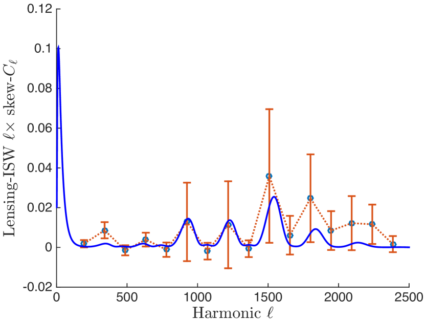
We see that temperature results from the full mission are consistent with the 2013 nominal mission (Planck Collaboration XXIV 2014). Including polarization yields results that also appear consistent and decrease the error bars. However, for now the T+E conclusions should be considered preliminary, for the reasons related to polarization data discussed in detail in Sects. 6 and 7. The error bars will also improve when measured with the other bispectrum estimators. As already seen in 2013, the values for are slightly low compared to the expected value of 1, but not significantly so. On the other hand, the detection of the lensing-ISW bispectrum is significant, even with our conservative rescaling of the error bars. The hypothesis of having no lensing-ISW bispectrum is excluded at using temperature alone, and improves to with the current preliminary result when including polarization. As mentioned above, the latter result is likely to improve with further analysis of the Planck data. In Fig. 1 we present the results of the skew- analysis for lensing-ISW NG for the map, which illustrates that the instrument and data processing are not removing this expected NG signal from the data.
4.2 Non-Gaussianity from extragalactic point sources
The auto-bispectra of extragalactic point sources are a potential contaminant to primordial NG estimates at Planck frequencies. The basic modelling and methodology of this section follows the corresponding section in Planck Collaboration XXIV (2014).
Extragalactic point sources are divided into populations of unclustered and clustered sources. The former are radio and late-type infrared galaxies (see e.g., Toffolatti et al. 1998; González-Nuevo et al. 2005), while the latter are dusty star-forming galaxies constituting the cosmic infrared background (CIB; Lagache et al. 2005). The contamination due to both types of sources in NG estimators is handled via dedicated bispectrum templates which are fitted jointly with the primordial NG templates.
The unclustered sources have a white noise distribution, and hence constant polyspectra. Their reduced angular bispectrum template is thus
| (55) |
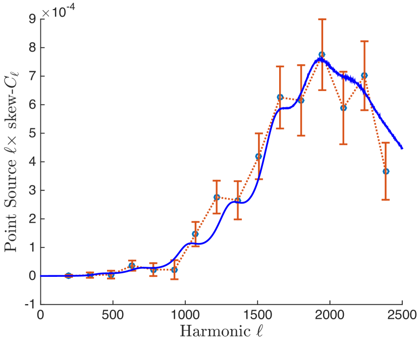
This constant is usually noted or in the literature (e.g., Komatsu & Spergel 2001). This constant template is valid in polarization as well as temperature, since the polarization angles of point sources are less clustered than the source density. However, since not all these point sources are polarized, we do not measure the same sources in temperature and in polarization. In fact, there is no detection of the bispectrum of unclustered point sources in the cleaned Planck polarization map, unlike in the temperature map, where Table 3 (binned bispectrum estimator) and Fig. 2 (skew-s) show a clear detection.
The clustered sources (CIB) have a more complex bispectrum in temperature, reflecting the distribution of the large-scale structure and the clustering of galaxies in dark matter halos (Argüeso et al. 2003; Lacasa et al. 2012; Crawford et al. 2014). The Planck results have allowed the measurement of the CIB bispectrum at frequencies 217, 353, 545 GHz in the range (Planck Collaboration XXX 2014). In this multipole range, a power law was found to fit the measurement, with an exponent consistent between frequencies. However, at lower multipoles theoretical models for the CIB power spectrum (e.g., Planck Collaboration XXX 2014) and bispectrum (Lacasa et al. 2014; Pénin et al. 2014) predict a flattening of the CIB power. We thus take the TTT CIB bispectrum template to be a broken power law,
| (56) |
where the index is , the break is located at , and is the pivot scale for normalization. Dusty star-forming galaxies emit with a low polarization fraction, and polarization correlates only over the smallest scales, so that the CIB is negligibly polarized. We thus take vanishing templates for its polarized bispectra
| (57) |
Both point source templates, Eqs. (55) and (56), have been implemented in the binned bispectrum estimator described in Sect. 3. The results for these two templates applied to the Planck temperature map, cleaned with the four component separation methods, can be found in Table 3. Since the two templates are highly correlated, the results have been determined in a combined analysis. The results have also been determined jointly with the primordial local, equilateral, and orthogonal templates, and the lensing-ISW bias has been subtracted, but all of this makes a negligible difference. Contamination from unclustered sources is detected in all component-separated maps. However, is not detected.
|
The order of magnitude of the bispectrum amplitudes found in Table 3 is consistent with expectations. Indeed, for radio sources at 217 GHz and with a flux cut based on the Planck ERCSC (Planck Collaboration VII 2011), Lacasa & Aghanim (2014), the forecasted is approximately . For the CIB, the Planck 2013 measurement (Planck Collaboration XXX 2014) at 217 GHz gives when translated into dimensionless units. The results reported in Table 3 are consistent at the order-of-magnitude level with these estimates, although they are lower, because we are analysing cleaned maps.
The unclustered point source and CIB templates are highly correlated, at 93 %. For this reason it was not deemed a priority for the other bispectrum estimators to implement the CIB template as well. Moreover, both point source templates are negligibly correlated with the primordial NG templates and the lensing-ISW template (the maximum being the correlation between equilateral and CIB templates at 2.7 %, while correlations with the unclustered point source template are well below 1 %). For this reason, and despite the detection of point sources in the cleaned maps, it makes no difference for the primordial results if point sources are included in a joint analysis or completely neglected.
An additional contaminant to the cosmological CMB bispectrum arises from the correlation between the gravitational lensing of the CMB anisotropies and the CIB anisotropies. This correlation was detected in Planck Collaboration XVIII (2014) using an optimal cross-spectrum estimator. The CIB-lensing bispectrum might couple with any of the primordial shapes. However, the amplitude of the CIB bispectrum is predicted to be small in the cleaned Planck maps and it has actually not been detected (see Table 3). The CIB-lensing bispectrum signal is frequency dependent, and it is mostly dominant in the very high Planck frequencies (see e.g., Curto et al. 2014).
4.3 Non-Gaussianity from residuals of the deglitching processing
Cosmic rays interacting with the cryogenic detectors induce spikes in timelines. These high-amplitude, fast-rising signals are followed by a decay tail. We observe three families of glitches, characterized by their temporal shape. The amplitude and time constants of the decays depend on which part of the satellite is hit (Catalano et al. 2014; Planck Collaboration X 2014). These random events are Poisson-distributed in time and produce highly non-Gaussian systematics.
A method has been developed to remove them directly at the time-ordered information (TOI) level. This process is performed iteratively, and is described in detail in Planck Collaboration X (2014). The short glitches are just flagged in the data, whereas for the long ones only the fast part is flagged, and the long tail is substracted from the timeline. This procedure is not perfect, and there are residuals from the potentially biased errors in the fit, and the undetected glitches under the threshold of of the TOI noise rms. They could in principle produce a non-Gaussian signal in the final map. In addition, these residuals could interact with the mapmaking procedure at the destriping level, since the error on the offset determination could be non-Gaussian due to undetected glitches or a possible bias in the errors of the removal of tails. This is important, because in more than of the TOI data, tails have been subtracted.
To estimate the effect of these residuals on the determination of NG, we created two sets of simulations (one including glitches and the other not) for every bolometer of the 143 GHz channel. We generated Gaussian CMB maps, and applied the full TOI processing with a realistic instrumental noise (Planck Collaboration VII 2016). In the simulations with glitches, we added glitches at the TOI level, following the properties measured in the data, and cleaned them with the procedure applied to the data. For the simulations without glitches, we have the same CMB and noise realization, but no glitches added at the TOI level.
We estimated the bias caused by glitches on the measurement of using the binned bispectrum estimator. The bias on induced by the glitch residuals on a map , including noise and CMB is given by , where the noise in the weighting of the estimator is determined from the simulations with glitches (as it would be for the data). Results are shown in Table 4. For most shapes, we detect no significant bias. The higher signal and high dispersion for the local shape might be due to a mis-calibration of the linear correction. In any case, for all shapes the bias due to glitches is a negligible correction to the value of , given its error bars, and we will not take it into account in the remainder of the paper.
|
5 Validation tests
During the work for the 2013 release, culminating in the NG results of Planck Collaboration XXIV (2014), the advantage of having multiple independent bispectrum estimator implementations was amply demonstrated. This allows for very useful cross-checking of results, both during development and for the final analysis, thus greatly improving the robustness of and confidence in the final results. For this new release we followed the same procedure, with the same three principal bispectrum estimators: KSW; binned; and modal, all of which had their pipelines updated to handle polarization data in addition to temperature.
Beyond the usefulness of cross-checking, the three estimators complement each other and have different strengths. The KSW estimator can treat separable bispectrum templates without approximation, but it is more work to add new templates and non-separable templates cannot be handled at all. The binned and modal estimators can reconstruct the full bispectrum (smoothed in different domains), while the skew- extension of the KSW estimator can be used to investigate the bispectrum beyond . The binned bispectrum estimator is the fastest on a single map or a set of unrelated maps, but becomes slower than the other two on a large set of realizations based on the same settings, because the linear correction term cannot be precomputed. The modal estimator can investigate a wide selection of oscillating or otherwise rapidly changing bispectrum templates that would be difficult to bin, while the binned bispectrum estimator can quickly implement and determine the of an additional template or the effect of a different cosmology if the binned bispectrum of the maps has already been computed. The binned estimator gets the dependence of on for free with its results, while the modal estimator allows for a statistical investigation of the mode coefficients.
In this Section we show some of the validation tests, in particular for polarization. In Sect. 5.1 we investigate the agreement between estimators, map-by-map, on sets of successively more realistic maps. In Sect. 5.2 we show that the estimators are unbiased in the presence of a non-zero . Finally, in Sect. 5.3 we show that the estimators are essentially optimal on a set of the most realistic Planck simulations available, which are those used to compute the error bars on our final results.
5.1 Agreement between estimators on a map-by-map basis
The maps used in this subsection are realistic simulations of the CMB (at resolution ) but without any foregrounds. They do not contain any primordial NG, but do include ISW-lensing. Since the final FFP8 simulations were not yet available, the main goal was to make sure that the estimators agreed with each other, not only on average, but also on a map-by-map basis. For this purpose it was enough to look at only 49 maps. Establishing optimality of the estimators requires a larger number of maps, and is shown on the FFP8 simulations in Sect. 5.3.
In our first test we include the effect of the 143 GHz beam, but in other respects the simulations are ideal (no noise, and no mask). The analysis used for both T and E. The results for the average over the maps for the KSW, binned, and both modal estimators, as well as for the difference between each estimator and KSW, are shown in Table 5. The shapes are assumed to be independent in this analysis, which means that the bias on the local shape due to the ISW-lensing effect is clearly visible. Results are shown for T-only, E-only, and the full combined T+E analysis. Note that the second modal implementation cannot compute results for E alone. One clearly sees that the results agree very well. It is also interesting to note that in this ideal noiseless case, one can actually determine more accurately from polarization alone than from temperature alone. This is due to the narrower transfer function in polarization, so that the primordial bispectrum is less smoothed in its projection to two-dimensional harmonic space.
|
||||||||||||||||||||||||||||||||||||||||||||||||||||||||||||||||||||||||||||||||||||||||||
The second test is identical to the first, except that we add realistic anisotropic noise realizations to the full-sky maps, based on the 143 GHz channel. The estimators now require the use of the linear correction term, and results are shown in Table 6. The agreement is still very good, although slightly worse than in the ideal case, as expected. The fact that the error bars for the T-only local case here are actually a bit smaller than in the ideal case is an artefact of the small number of maps; i.e., the error bars have not completely converged yet. On the other hand, the fact that the error bars for E-only are much larger than in the ideal case is a real effect; the Planck single-frequency polarization maps are noise-dominated.
| Shape . KSW Binned Modal 1 Modal 2 B KSW M1 KSW M2 KSW T Local . 6.7 4.8 6.4 5.2 6.7 4.7 7.0 5.3 0.3 1.0 0.1 0.4 0.3 1.2 T Equilateral . 11 61 12 65 9 63 12 62 1 15 1.9 9.6 1 12 T Orthogonal . 19 31 18 34 20 32 18 35 1 12 1.3 5.1 0.8 8.8 E Local . 2 29 4 28 1 29 2 12 0.4 5.5 E Equilateral . 1 191 18 195 6 200 19 47 7 23 E Orthogonal . 6 101 0 107 6 102 6 25 0.3 10 T+E Local . 4.9 4.2 4.5 4.4 5.0 4.2 4.9 4.9 0.4 1.2 0.1 1.5 0.0 1.2 T+E Equilateral . 13 46 11 49 9 48 13 47 2 10 4 13 0.3 7.0 T+E Orthogonal . 11 22 11 24 13 22 11 24 0.0 7.3 1.3 7.1 0.7 4.5 |
Finally, the third test is identical to the second, except that we now also add a mask. The mask chosen is realistic, based on the union of the confidence masks provided by the SMICA, NILC, SEVEM, and Commander methods for this particular set of simulations. It contains both a Galactic and a point source part. The temperature mask leaves 79 % of the sky unmasked, while the polarization mask leaves 76 %. The results are shown in Table 7, while the map-by-map comparison is given in Fig. 3. From the table we see that the agreement between the different bispectrum estimators is still very good and only slightly degraded when compared to the previous case. The typical discrepancy between the bispectrum estimators, even in this most realistic case, is less than about a third of the uncertainty on . This is apparent in the map-by-map comparison of Fig. 3.
|
||||||||||||||||||||||||||||||||||||||||||||||||||||||||||||||||||||||||||||||||||||||||||
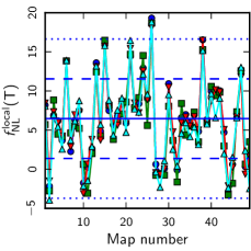
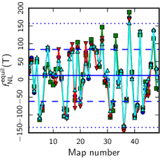
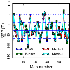
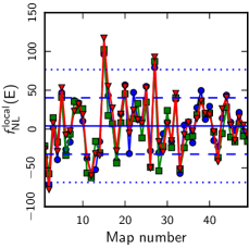
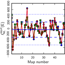
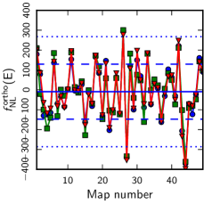
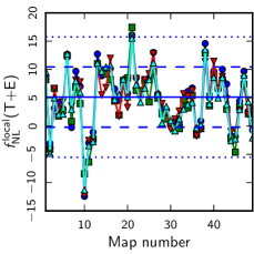
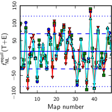
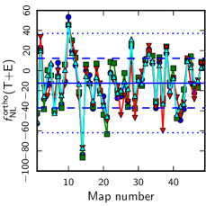
5.2 Validation of estimators in the presence of primordial non-Gaussianity
After the map-by-map comparison of the previous section, we next want to make sure that the estimators are unbiased. For this purpose we prepared a different set of 100 T and E CMB simulations, still with cosmological parameters as determined by Planck. This time ISW-lensing is not present, but there is a nonzero local . To these maps we add the same beam, anisotropic noise, and mask as before. We again take , and the results are given in Table 8.
We see that all the estimators correctly recover the input value, both in temperature and in polarization. The results for the equilateral and orthogonal shapes are consistent with the fact that those templates have a non-zero correlation with the local shape (the Table gives the results for an analysis where all shapes are assumed independent). For example, a joint analysis of the T+E binned estimator gives , , and . Except for the first modal estimator in E-only (due to an insufficient number of maps in the linear correction term), we also find that the error bars for the bispectrum-based estimators are very close to the Fisher errors. Note that a slight increase in the error bars compared to Fisher estimates is expected for the local shape in T-only and in T+E, due to the signal being significantly different from zero there (the Fisher error bars for the local case are 5.8 for T-only, 26 for E-only, and 5.0 for T+E). Hence the estimators are effectively optimal, as will be illustrated in more detail in the next section.
|
||||||||||||||||||||||||||||||||||||||||||||||||||||||||||||||||||||||||
5.3 Validation of estimators on realistic Planck simulations
As a final validation test, we ran our estimators on a large set of the most realistic simulations available. These are the FFP8 simulations (Planck Collaboration XII 2016) using SMICAfor foreground separation. They are the same simulations we use to determine the error bars on our final SMICA results in Sect. 6. They contain the Collaboration’s best estimates of the CMB sky and of Planck’s noise and beam effects, and have been cleaned by SMICA in the same way as the real sky map. The mask used is the same common mask defined for the real data analysis. For this test the estimators were all processed with the same settings used for the final data analysis.
Here we take 159 of these maps, and process these using all the estimators. By contrast, for the final results in Sect. 6, the convergence of the error bars of each estimator was carefully checked, using more maps if required. This explains why there are some small differences between the error bars in Sect. 6 and the ones presented here.
| Shape . KSW Binned Modal 1 Modal 2 Mink.F. B KSW M1 KSW M2 KSW MF KSW T Local . 7.1 5.5 7.0 5.4 6.2 5.5 6.3 6.2 7 12 0.1 1.1 0.9 1.9 0.8 1.9 0 11 Equilateral . 2 67 4 67 4 73 5 66 2 19 6 32 3 18 Orthogonal . 23 32 24 33 24 33 20 36 1 11 0.9 9.1 3 14 E Local . 0.5 32 0 35 1 30 0 49 0.8 8.3 0.7 8.3 0 37 Equilateral . 7 144 7 143 9 152 0 37 2 35 Orthogonal . 5 72 7 75 4 73 2 22 1 17 T+E Local . 5.6 5.1 5.0 4.9 4.7 4.8 4.3 5.3 5 11 0.6 1.2 0.9 1.5 1.3 1.7 1 11 Equilateral . 3 46 5 44 3 46 4 43 2 14 0 14 1.0 9.7 Orthogonal . 10 22 9 22 9 21 7 22 0.8 7.0 0.8 7.3 2.7 7.7 |
The results are shown in Table 9. Note that these are the results from an independent analysis, without subtracting the ISW-lensing bias. We also show the results from Minkowski functionals (for the local case only).131313Since the Minkowski-functional pipeline automatically subtracts the ISW-lensing bias, the theoretical value for the bias as computed from the Fisher matrix has been added to its results, to make a direct comparison possible. We see that there is very good agreement between the bispectrum estimators even on this most complex and realistic set of simulations. The standard deviation of the difference between bispectrum estimators generally stays below one third of the error bar on , the only exception being the T-only equilateral result for the Modal 1 pipeline, which is still smaller than one half of the error bar. We see that the results from Minkowski functionals are consistent, but clearly suboptimal for . They are however a valuable, independent check.
The exact Fisher error bars for the nine shapes considered in the table are, in the same order as the table: 5.4, 69, 35; 31, 131, 74; 4.7, 43, 21. Taking into account the relative error in the standard deviation of , which is for 159 maps, we see that all bispectrum estimators are effectively optimal on all shapes, except for the E-only equilateral case where they appear slightly suboptimal. The small suboptimality of the Modal 2 pipeline for the local shape seen here disappears once more maps are used (see the results in Sect. 6).
In conclusion, all these validation tests show that we have very good agreement between the results from the different bispectrum estimators, not just on average, but also on a map-by-map basis. In addition we see that, despite the approximations made in the pipelines, and the simple treatment of the masked part of the maps (diffusive inpainting method and factor), the bispectrum estimators we use are all essentially optimal.
6 Results
6.1 Constraints on local, equilateral, and orthogonal
In this section we investigate the local, equilateral, and orthogonal primordial templates. These are now established as the standard shapes to study first when investigating the bispectrum (see Sect. 2 for a theoretical motivation and description of these shapes). However, they represent only the tip of the bispectral iceberg, and many more shapes are investigated in Sect. 8, while full model-independent reconstructions of the bispectrum are presented in Sect. 6.2.
For a complete description of the Planck data set and the bispectrum estimator configurations we have used, we refer the reader in particular to Sect. 3.4 and Sect. 3.5. To summarize the overall analysis methodology, we have employed four independent bispectrum estimators on the full mission Planck temperature and polarization maps obtained from the four different component separation pipelines, SMICA, SEVEM, NILC and Commander. The bispectrum estimators are the KSW estimator with its skew- extension using exact separable templates (Sect. 3.1), the Binned estimator using fixed multipole bins (Sect. 3.3), and the Modal 1 and Modal 2 estimators, which both use separable eigenmode expansions (Sect. 3.2). Temperature is analysed over the multipole range to or above and polarization is analysed from to or above (Sect. 3.5). By employing inpainting and a linear term, all these estimators essentially achieve optimality (as shown by comparison with Fisher matrix forecasts). The linear term in Eq. (3) and the uncertainties are determined using the FFP8 simulations (Sect. 3.5), also processed through the different foreground-separation pipelines. Our thorough validation campaign for these estimators is presented in Sect. 5.
The results of the analysis of the four cleaned maps with the four estimators, for T-only, E-only, and full T+E, are shown in Table 10, which is one of the main results of this paper. Results are determined while assuming all shapes to be independent, and are shown both with and without subtraction of the ISW-lensing bias (see Sect. 4.1 for more details about ISW-lensing). This bias is most important (relative to the size of the error bars) for the local shape, but also non-negligible for the orthogonal shape. Results here have not been marginalized over the point source contributions. While Sect. 4.2 shows that there is still a significant contamination by unclustered point sources in the cleaned maps, the correlation with the primordial templates is so small that this has no impact on the results reported here (as checked explicitly).
While Table 10 is the main result of this Section, in order to simplify the use of the Planck results by the wider scientific community, we also present in Table 11 the results that can be considered the final Planck 2015 results for the local, equilateral, and orthogonal shapes. As in 2013, we select the combination of the KSW estimator and the SMICA map for this. The SMICA map consistently performs well in all data validation tests, which are discussed in detail in Sect. 7. The KSW estimator, while unable to deal with non-separable templates, treats separable templates exactly, and the local, equilateral, and orthogonal template are all separable. On the other hand, the binned and modal estimators can deal with non-separable shapes and have other advantages as well (like full bispectrum reconstruction), but at the price of using approximations for the templates. However, they have all been optimized in such a way that the correlation with the exact templates for the three primordial shapes is close to perfect, so that in the end the results by the different estimators are statistically equivalent. Compared to the corresponding values in Table 10, the difference in the numbers in the last column of Table 11 is due to the fact that in the latter the equilateral and orthogonal have been determined jointly.
Focusing on the results for temperature-only and the full temperature plus polarization (T+E) results, we see that there is no evidence for a non-zero bispectrum with any of these three primordial shapes (local, equilateral, and orthogonal). After ISW-lensing subtraction, all values are consistent with at CL. The temperature results are all very similar to the ones from the nominal mission data published in 2013 (Planck Collaboration XXIV 2014), with very minor improvements in the error bars due to the additional temperature data. We also see that results are quite consistent when including polarization, with error bars shrinking by about 15 % for local, 35 % for equilateral, and 40 % for orthogonal.
Table 10 displays very good agreement between the results from the different estimators, at the level expected from the validation tests in Sect. 5. We also note how the error bars, which are determined using the FFP8 simulations, are statistically indistinguishable from the optimal Fisher expectation.
Different component separation methods also show a good level of agreement when looking at temperature-only and combined temperature plus polarization results. The accuracy of this statement will be shown and quantified in detail in Sect. 7. However, in the same section, we will also show how the agreement between extracted from different cleaned maps becomes significantly degraded when considering polarization-only results141414The E-only agreement is still at a reasonable level in most cases. However this is larger than expectations from simulations, as described in Sect. 7.. The reasons behind this loss of internal consistency are not fully understood at present. Polarization data are, however, much noisier than temperature data, implying that the EEE bispectra have a close to negligible weight in the final combined measurement, which is dominated by the TTT and TTE configurations. In fact, as just mentioned above, the combined measurement looks perfectly self-consistent: local, equilateral and orthogonal measurements in the T+E column of Table 10 pass all our tests of robustness.
We can thus conclude that, while highly challenging from a technical point of view, the inclusion of polarization in our estimator pipelines has been a success, allowing for a significant tightening of the constraints on the three standard primordial bispectrum shapes. On the other hand, in light of the outstanding issues in E-only results, we present our results conservatively, and recommend the reader to consider all constraints that make use of polarization data throughout this paper as preliminary at the current stage. We stress again that this is a conservative choice, which is made despite the fact that no test to date shows any evidence of leakage of the issues in EEE bispectra into the T+E measurements. A detailed description of all the data validation tests, which lead to the robustness-related assessments summarized here, can be found in Sect. 7 (for readers less interested in the technical details, the main results and conclusions of all these tests are summarized in Sect. 7.6).
|
|||||||||||||||||||||||||||||||||||||||||||||||||||||||||||||||||||||||||||||||||||||||||||||||||||||||||||||||||||||||||||||||||||||||||||||||||||||||||||||||||||||||||||||||||||||||||||||||||||||||||||||||||||||||||||||||||||||||||||||||||||||||||||||||||||||||||||||||||||||||||||||||||||||||||||||||||||||||||||||||||||||||||||||||||||||||||||||||||||||||||||||||||||||||||||||||||||||||||||||||||||||||||||||||||||||||||||||||||||||||||||||||||||||||||||||
|
||||||||||||||||||||||||||||||||
6.2 Bispectrum reconstruction
6.2.1 Modal bispectrum reconstruction
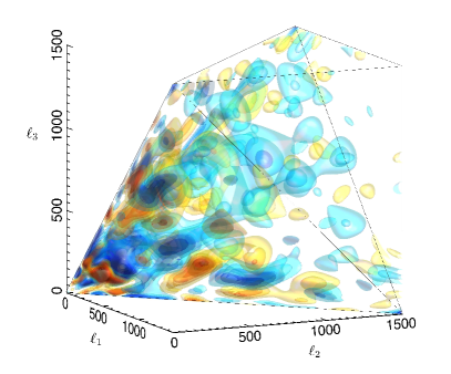
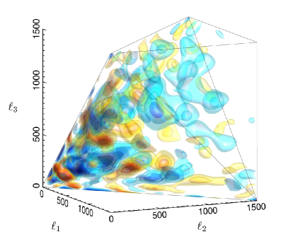
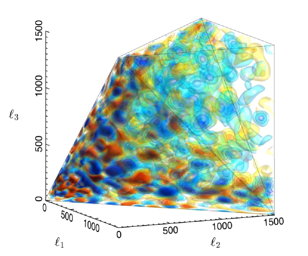
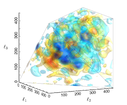
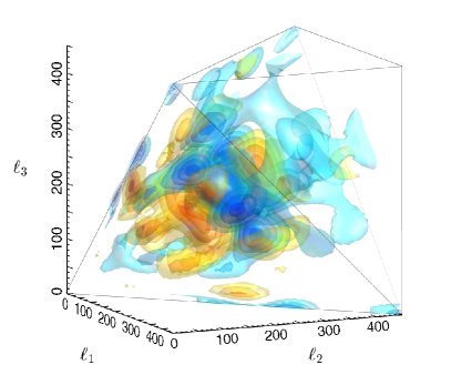
The starting point for modal bispectrum estimation is the robust extraction of the modal coefficients from each of the full mission foreground-separated maps, that is, SMICA, SEVEM, NILC, and Commander. The -coefficients are obtained for each of the temperature, polarization, and mixed bispectrum components, TTT, TTE, TEE, and EEE. Their cross-correlation between cleaning methods is an important validation of their accuracy, as we shall discuss in the next section, with excellent correspondence for temperature and some differences remaining in polarization. The modal basis number for the full mission analysis has been substantially increased offering a higher effective resolution when compared to the 2013 Planck Data Release where modes were used. Several different basis functions have been used, including trigonometric functions, sinlog basis functions, and polynomials (closely related to Legendre functions), with the latter chosen because of excellent convergence in the squeezed and flattened limits.
We can reconstruct the full three-dimensional Planck bispectrum, obtained using these basis functions, to visualize its main properties and to determine robustness. A comparison between the temperature-only bispectra from the Nominal Mission and full mission at the same modal resolution is shown in Fig. 4. Note the excellent agreement with all the main features replicated in the new data. In Fig. 4 in the third bispectrum, we also demonstrate the much higher bispectrum resolution achieved with the full modes. The tetrapyd shape reflects the constraints on the wavenumbers , and , with the squeezed configuration appearing on the axes that lie along one . The expected ISW-lensing bispectrum is an oscillating signal in the squeezed limit along the tetrapyd edges; it is now measured with a significance of (see Sect. 4.1). This ISW-lensing signal sets an interesting benchmark or threshold against which to compare the other strong features observed in the bispectrum and now defined with greater precision. The original “plus-minus” feature, with a large positive red peak around followed by a larger negative peak near , remains though with more substructure, together with a broad negative peak in the equilateral limit around , which can be associated with the third acoustic peak from the transfer functions. Oscillatory models, which can connect these three peaks, achieve higher significance. The apparent signal observed in the flattened limit remains, with a distinct pattern of blue and red features on the surface of the tetrapyd.
We also include a comparison with WMAP-9 in Fig. 5, where we have restricted the reconstructions to for comparison with modes. These plots, using identical isosurfaces, show the same bispectrum structure including the “plus-minus” feature clearly bisecting the main peak and the first oscillation of the ISW-lensing bispectrum visible along the lower tetrapyd edges. The WMAP-9 reconstruction only shows significant differences from Planck in the top right region, where the higher noise levels in WMAP-9 make its reconstruction less reliable.
All four components of the temperature and polarization bispectrum reconstruction obtained from SMICA are shown in Fig. 6. A direct comparison of the EEE polarization bispectrum for SEVEM, NILC and Commander, is shown in Fig. 7, where we note that these are orthogonalized E-mode contributions (see the Modal 2 discussion in Sect. 3). It is interesting to observe patterns of features evident in the polarization bispectra from the different foreground-cleaned maps, which, although inherently noisier, have qualitative similarities. At a quantitative level, however, the polarization bispectra modes from different methods are less correlated in polarization than in temperature, as we discuss in Sect. 7.
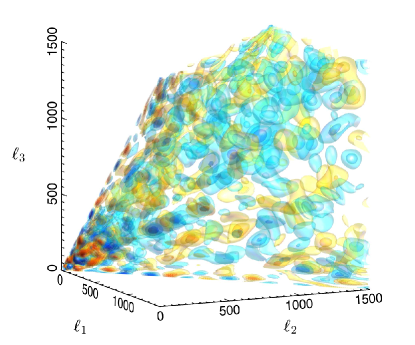
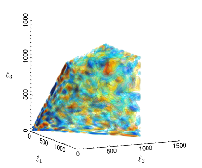
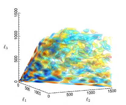
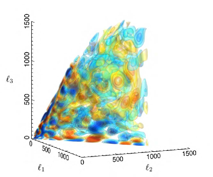
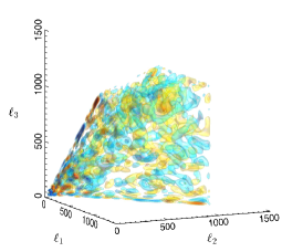
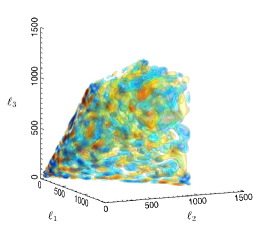
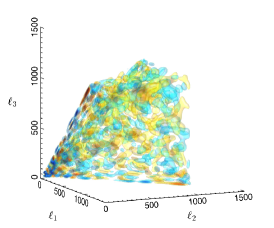
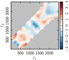
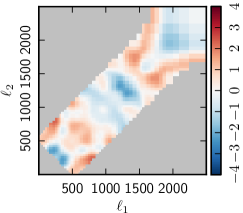
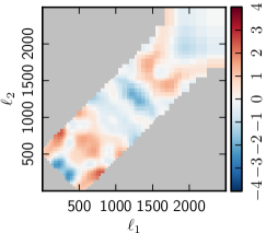
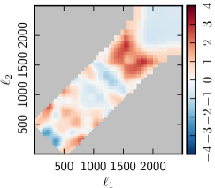
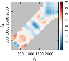
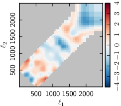
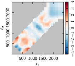
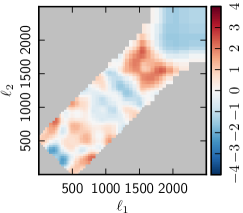
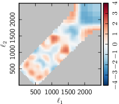
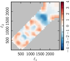
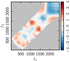
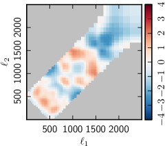
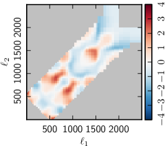
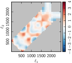

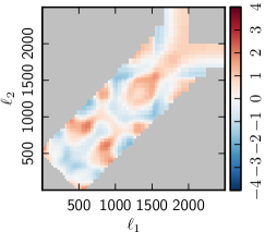
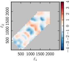
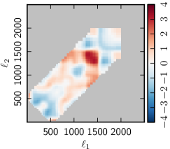
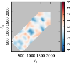
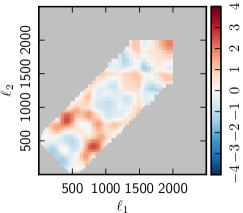
6.2.2 Binned bispectrum reconstruction
The (reconstructed) binned bispectrum of a given map is a natural product of the binned bispectrum estimator code (see Sect. 3.3). To test if any bin has a significant NG signal, we study the binned bispectrum divided by its expected standard deviation, a quantity for which we will use the symbol . With the binning used in the estimator, the pixels are dominated by noise. We thus smooth in three dimensions with a Gaussian kernel of a certain width . To avoid edge effects, due to the sharp boundaries of the domain of definition of the bispectrum, we renormalize the smoothed bispectrum, so that the pixel values would be normal-distributed for a Gaussian map.
In Figs. 8 and 9, we show slices of this smoothed binned signal-to-noise bispectrum with a Gaussian smoothing of , as a function of and . Very red or very blue regions correspond to a significant NG of any type. The two figures only differ in the value chosen for the -bin, which is for the first figure, and for the second. We have defined two cross-bispectra here: ; and . These two cross-bispectra are then divided by their respective standard deviations (taking into account the covariance terms) to produce the corresponding and . Those three different permutations are not equal a priori due to the condition , which is implemented in the code to reduce computations by a factor of six. However, part of the smoothing procedure involves adding the other five identical copies, so that in the end the plots are symmetric under interchange of and (and is symmetric under interchange of all its indices). The grey areas in the plots are regions where the bispectrum is not defined, either because it is outside of the triangle inequality, or because of the limitation . Given that in both plots is fixed at less than 2000, is not defined if both and are larger than 2000, while is undefined if either or (or both) are larger than 2000.
Results are shown for the four component separation methods SMICA, SEVEM, NILC, and Commander, and for TTT, T2E, TE2, and EEE. In addition we show on the second line of each figure the result for TTT with the radio (unclustered) and CIB (clustered) point source bispectra subtracted according to their jointly measured amplitudes. It is clear, in particular in the second figure, that at higher there is a very significant point source contamination in the cleaned TTT bispectra, in agreement with the results of Table 3. However, after removing it we do not see a clear signal of any other residual NG. Of course this is for the moment only a qualitative statement; more quantitative tools for studying the amount of NG in these smoothed bispectra are in development.
Looking at the polarized bispectra in the high- slices, in particular TE2 and EEE, we do see some bluer and redder regions that might indicate residual NG. This agrees with statements made earlier, and discussed in greater detail in the next section, that the Planck polarized bispectrum is for the moment not as clean and well-understood as the temperature one. We also see a very good qualitative agreement between the four component separation methods in temperature, which worsens somewhat when mixing in more and more polarization; in particular SMICA and NILC give very similar results.
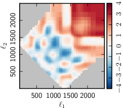
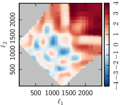
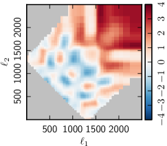
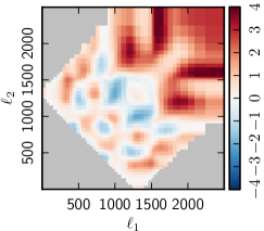
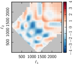
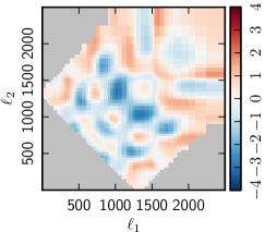
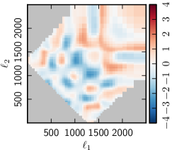
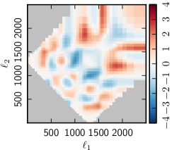
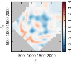
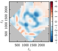
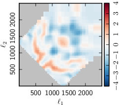
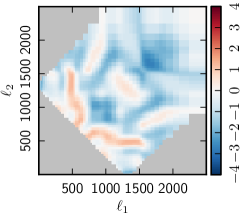
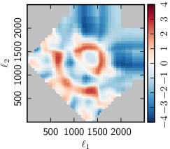
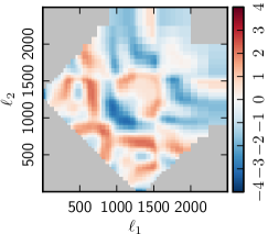
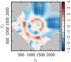
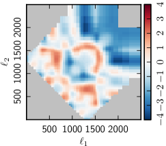
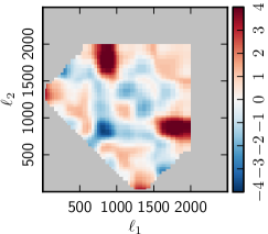
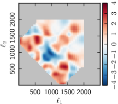
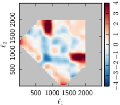
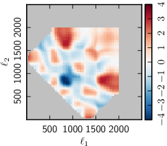
6.3 Primordial Curvature Reconstruction
In this section, we compress the information in and maps into maps of projected primordial curvature fluctuations, . To the extent that the primary CMB temperature and polarization are Gaussian fields and the early universe fluctuations are presumed Gaussian, all of the information in is encoded in the mean field (Wiener-filtered map) plus fluctuations, characterized by a covariance matrix; it is just a different compression/re-expression of the original statistics. Thus, one could look for non-Gaussian deviations by directly evaluating the 3-point and higher statistics of this re-expression. Since fluctuations as well as the mean are given, a full description of the errors follows. That a Gaussian assumption is made does not mean that the Wiener-filtered map is in fact Gaussian, since the constraining data may drive it from a map consistent with Gaussianity. Hence one can search in the statistics of the Wiener-filtered map for evidence for non-Gaussianity.
The weighting of the temperature and -mode polarization associated with the Wiener filter is an optimal one (inverse-total-covariance weighted), and estimators for non-Gaussianity constructed using this expression are nearly optimal. However, since a (fiducial) primordial power spectrum is assumed for the Wiener filter (usually a uniform -spectrum, using the best fit Planck 2015 scalar spectral index and power amplitude ), this approach is best suited for perturbative non-Gaussianity of the sort we treat in this paper. In practice, the estimators used here for non-Gaussianity act directly on temperature and polarization data, rather than through the intermediary of optimal -maps and their fluctuations.
The scalar fluctuations can be expressed in terms of the curvature variable on uniform total density hypersurfaces, where is the inhomogeneous expansion factor, or, equivalently, by its wavenumber transform . In turn, can be expanded in multipoles, . Instead of the magnitude of the wavenumber , a mixed representation gives a multipole expansion at each comoving distance from our location, , , . Here or , with referring to the real part of and to the imaginary part. For there is no component, only . The mean of the field given the temperature field and its covariance describing allowed fluctuations about that mean are
| (58) | |||||
| (59) | |||||
In these expressions, is the total covariance for the temperature, including both signal and noise variances. The specific forms assume the matrix is diagonal in multipole space, depending only on , but if the noise is inhomogeneous it will have off-diagonal components and the equations become matrix equations. In this section, we assume the noise is diagonal. Eq. (58) shows the unsurprising result that for each only one mode is determined by . Replacing by gives and . Although and are correlated, the uncorrelated part of delivers a different mode for from the one given by . Thus when is constrained by both and , the two modes deliver substantially more information than for and alone, and the fluctuations about the mean are thereby diminished. This is further helped by the acoustic oscillations of polarization being out of phase with those for , so when is down, is not, and vice versa. The interplay of the two modes is quantified by signal-to-noise in Fig. 10.
When both and are included as constraints, a two by two matrix appears which includes the correlation in the off-diagonal as well as the and along the diagonal:
| (63) | |||
| (67) |
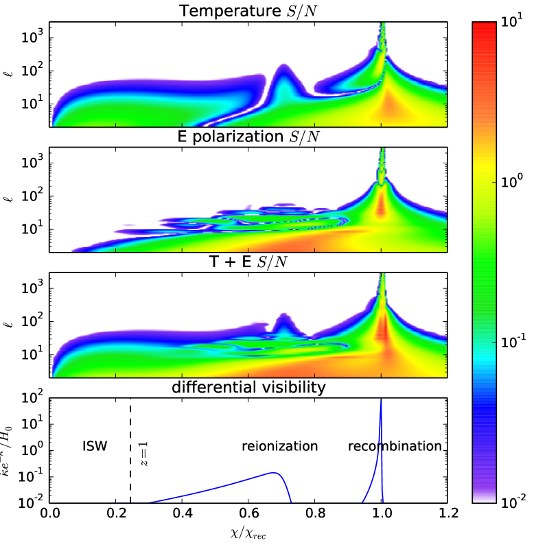
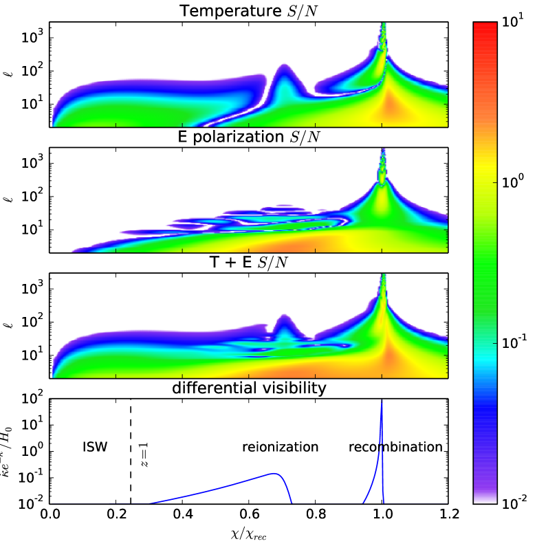
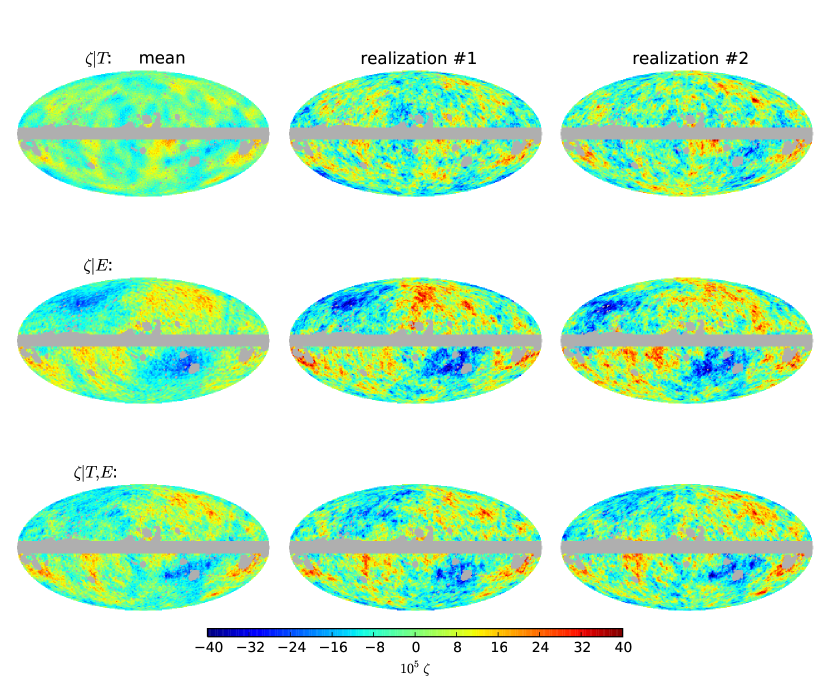
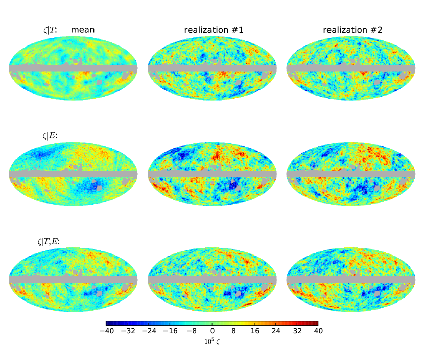
Fig. 11 shows an all-sky mean field (Wiener-filtered) map of the curvature variable constructed in (densely-packed) shells from the multipoles . The figure actually shows projected onto differential visibility, . The map is the spherical transform of . The top left map is using the all-sky maps SMICA DX11. The middle left map is , based on just the polarization information. (The E-maps did not have high pass filtering imposed, so that an indication of the full results obtainable with E alone can be seen.) The bottom left panel shows . Visually the combined two-mode constraint has more detail than either of the one-mode constrained maps, enhancing the estimation of . In each of the three cases, two sample realizations are shown which include allowed fluctuations about the mean map. These illustrate the level of uncertainty in the patterns found in the mean maps, necessary ingredients to the full statistical description. Note that the fluctuations about the mean are larger for or alone than for the combined .
In all cases, the fluctuations become very large indeed if we allow for arbitrary projections, not conditioned by the visibility. Another approach similar to the differential visibility projection is to make a slice at ; i.e., making the projection a delta-function in at the peak where , which defines . This single slice case is shown in Fig. 12. The figures look quite similar in structure to the projected differential visibility plots. Although is where most information is, the fluctuations of a single slice are somewhat larger than for the differential visibility projection. The differential visibility includes a subdominant “reionization bump”, with a small weight focused at low where sample variance is large; restricting the projection of to be just over the reionization region results in a low mean map that is largely swamped by the allowed fluctuations about it. The fluctuations about the mean become much larger if we project over all , since there are vast terrains in in which there is very little CMB temperature or polarization information; in particular between recombination and reionization. For that uncharted territory, a realization of the reconstructed -map reverts to a realization of the fiducial -power.
Fig. 10 quantifies where the information resides in – space. Here, the signal variance is the ensemble average of the square of the mean field, assuming the are drawn from a Gaussian with fiducial covariance,
| (68) |
and the noise (i.e., fluctuation) variance is the covariance matrix, as given by Eq. (6.3) for and the equivalent for . Fig. 10 plots the signal-to-noise at each individual slice (hence ignores the components off-diagonal in ):
| (69) |
for , with an equivalent expression for . The signal-to-noise structure in can be contrasted with the differential visibility plotted in the bottom panel: Fig. 10 shows that the – information has a reach beyond the differential visibility structure, especially for low multipoles, because the associated waves can straddle the last scattering surface. The “reionization bump” in signal-to-noise seen in Fig. 10 is not that prominent. The Integrated Sachs Wolfe impact on the S/N is evident, but is relatively low, with the consequence that we cannot draw out high significance results from the ISW effect for reconstruction (or equivalently for gravitational potential reconstruction).
The top panels in Fig. 10 are for an ideal experiment, with no noise (apart from the cosmic variance “noise” in the Wiener map fluctuations). The bottom panels of Fig. 10 include realistic Planck noise, as estimated from the FFP8 simulations: the high signal to noise in in the top panels is noticeably diminished around over what a cosmic variance limited experiment would give.
Figs. 11 and 12 are Gaussian-filtered on a relatively large scale ( FWHM). To see what happens at higher resolution, Figs. 13 and 14 zoom in on a typical patch, with long waves removed using a filter for . The specific choices are and , the values used for the Planck high pass for polarization maps. To allow direct comparison, we have just done the same high pass filtering for the map. We also removed the means of the maps. The resolution is ( FWHM). Figs. 13 and 14 illustrate that the fluctuations play a larger role in this higher resolution regime. Note that the slice has about the same fluctuation level as the differential visibility projection.
Lensing effects are not taken into account in these -maps. In principle one could de-lens the temperature and polarization maps before forming the Wiener filter. In practice this would be a highly noisy operation with current Planck data. Hence the contaminating influence of lensing on these -reconstructions would be treated by comparing simulated -maps with and without lensing. Such corrections are expected to be a subdominant bias, as it has been modelled in the rest of the paper.
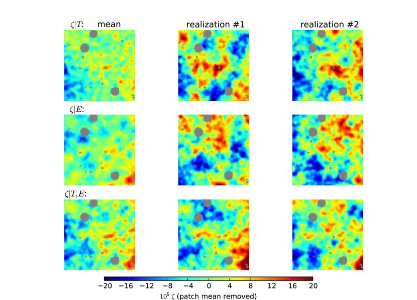
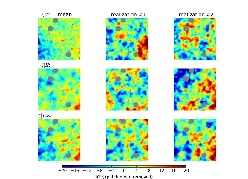
7 Validation of Planck results
In this section, we perform a battery of tests aimed at verifying the robustness of the results obtained in the previous section. Table 10 shows excellent agreement with our 2013 analysis of nominal mission data (Planck Collaboration XXIV 2014). The agreement using different component separation methods in temperature is also generally very good. Our focus here is thus on polarization bispectra. Redundancy is perhaps the most important element in our analysis, as far as robustness is concerned. We devote considerable attention to comparing the outcomes of different estimators and component separation pipelines, and assess their level of internal consistency. We also verify the stability of our results in the harmonic and pixel domains, by considering different sky cuts and multipole intervals. Given the large computational requirements of these tests, and since results from different optimal estimators agree very well, as shown in previous sections, we will variously use the KSW, binned, or modal pipeline for different tests. In doing this we will also exploit the complementarity of different decompositions, which might make some of them more suited for different tests than others (for example, the binned pipeline directly works with a harmonic space decomposition of the bispectrum, thus making it perfectly suited for tests of -dependence, the modal pipeline can perform quick model-independent tests by working on a relatively small subset of bispectrum modes, and so on).
7.1 Dependence on foreground cleaning method
7.1.1 Comparison between measurements
In Table 10 we show results for the local, equilateral and orthogonal shapes, using four different optimal estimators, and four different foreground cleaning pipelines. The agreement between different estimators, on a given map, is within a fraction of a standard deviation, in line with theoretical expectations and simulations, as reported in Sect. 5. This level of agreement applies to all of the T+E, (TTT), and (EEE) bispectra.
The overall picture becomes more complex when comparing outputs across different foreground cleaning methods and estimators. Whereas for TTT and T+E results the agreement also seems quite good in this case (being at the level of half a sigma or better, for nearly all combinations of cleaned maps and shapes), larger discrepancies are present in the EEE bispectrum measurements. The most notable differences are found for the equilateral shape, where SMICA and NILC find values of consistent with within , while SEVEM and Commander measure a roughly deviation from Gaussianity. The largest discrepancy is found for the pair Commander–NILC, using the binned pipeline (see table 10). This estimator recovers using the Commander E-map and using the NILC E-map. Other pipelines, and different choices of component separation methods, show slightly smaller but similar discrepancies, at a level of about . The same shape and estimator analysis of temperature maps shows good agreement: Commander recovers , while NILC gives . The combined T+E measurement, still for the same modal pipeline and equilateral shape, yields for Commander and for NILC, corresponding to about half a standard deviation difference. This general trend is seen for other shapes and estimators.
|
|||||||||||||||||||||||||||||||||||||||||||||||||||||||||||||||||||||||||||||||||||||||||||||||||||||||||||||||||||||||||||||||||||||||||||||||||||||||||||||||||||||||||||||||||||||||||||||||
Simulations were used to give insight into the expected level of disagreement. For each of the four component separation methods, we generated FFP8-based Gaussian simulations with realistic beams and noise levels. These simulations start from the same initial single frequency realizations, and are processed through the four different foreground cleaning pipelines. The starting maps do not include any foreground component (the same map generation procedure is used in the Monte Carlo determination of error bars). The differences in final simulations are thus generated only by the different data filtering and coadding operations performed either in pixel, harmonic, or needlet domains by the various foreground cleaning methods, and by additional manipulations of the maps which are required for estimation, such as inpainting. Therefore, the average scattering in , measured from these realizations, provides us with a baseline assessment of the expected discrepancies between different methods when foreground residuals and other spurious sources of NG are negligible. We can then compare them with differences observed on the data to establish whether they are consistent with expectations, or are too large. The latter would raise the concern that foreground contamination, or other systematics, might be affecting the results.
Results are shown in Table 12, for EEE and T+E and two different sky coverages. The scatter between values from simulations is about for both T+E and EEE. This is smaller than the differences in the Planck values obtained from EEE analysis of different foreground-cleaned maps, especially for the equilateral shape. However, for the final combined T+E measurement, observed differences are in good agreement with expectations from simulations for the majority of cases. Another important point is that the consistency shown in Table 12 for T+E measurements is stable to the change of sky coverage (in polarization) from to . This will be confirmed by additional tests later in this section. For the SMICA–SEVEM pair we also verified stability using an even larger mask with .
Residual foregrounds may be responsible for at least some of the observed excess of scatter in EEE-derived between different cleaning algorithms. This is supported by the fact that several EEE results for this test change significantly for different masks, and that discrepancies are alleviated by using a larger mask, especially for equilateral shapes (see e.g., SEVEM–NILC and SMICA–SEVEM in Table 12). However, modal coefficients and their correlations are stable to a change of mask (see below), as are values of for a given component separation method (see Table 13).
Another possible contributor is a mismatch between the noise model (used to build the estimator normalization, weights and linear term), and the actual noise in the data. Polarization data are very noisy, and it is a known problem that the model assumed underestimates the true noise. This means that the error bars for EEE results, quoted in Table 10, are somewhat underestimated, which does not seem to be a problem for the final T+E results, since the weight of the EEE bispectrum in the final combined measurement is very low. This is confirmed by the results of this test. Indeed, we investigate EEE in detail because it is a useful and sensitive indicator of various systematics in the polarized maps (which could eventually leak into the TTE and TEE bispectra), rather than for its statistical weight in the final measurement. It is then fair to say that issues in the EEE bispectra, and related measurements are not yet fully understood and will require further investigation. Even though the T+E are consistent, we recommend that results that include polarization data are regarded as preliminary at this stage.
| Difference Local Equilateral Orthogonal Local Equilateral Orthogonal Local Equilateral Orthogonal SMICA T. 6.8 5.4 17 66 48 33 E. 25 30 147 159 137 73 48 31 220 168 180 81 23 16 73 68 43 34 T+E. 4.0 4.8 5 46 30 21 4.6 5.2 19 55 37 22 0.7 1.2 14 14 6.7 7.7 SEVEM T. 8.1 5.8 11 75 49 34 E. 44 38 302 183 172 91 43 39 303 191 170 96 1 19 0 76 2 49 T+E. 6.4 5.0 15 52 44 23 6.2 5.3 31 54 50 25 0.2 1.3 16 15 6.3 8.8 NILC T. 6.4 5.8 31 76 50 33 E. 1 30 64 162 78 77 22 30 190 162 84 77 23 16 124 67 6 37 T+E. 3.3 4.9 15 50 27 23 4.0 5.3 1 56 33 23 0.7 1.3 16 13 5.4 7.5 Commander T. 6.4 6.6 3 77 49 36 E. 28 37 278 178 56 81 61 38 337 188 122 91 32 20 60 92 66 47 T+E. 5.2 5.4 30 50 39 23 6.0 5.7 45 55 51 25 0.7 1.5 15 14 11.5 8.9 |
| TTT EEE EEE Methods . Data Simul. Data Simul. Data Simul. SMICA–SEVEM. 0.97 0.97 0.61 0.62 0.60 0.61 SMICA–NILC. 0.97 0.97 0.95 0.95 0.95 0.95 SMICA–Commander. 0.78 0.81 0.70 0.70 0.73 0.73 SEVEM–NILC. 0.96 0.97 0.54 0.55 0.54 0.54 SEVEM–Commander. 0.81 0.83 0.69 0.67 0.70 0.70 NILC–Commander. 0.85 0.86 0.64 0.63 0.66 0.66 |
7.1.2 Comparison between reconstructed bispectra
It is important to stress that the conclusions reached at the end of the previous subsection refer to the three main bispectra in our analysis, defined by the standard scale-invariant local, equilateral, and orthogonal primordial shapes. These shapes select a specific subset of configurations in the overall bispectrum domain (essentially squeezed, equilateral, and flattened triangles). Therefore, testing consistency between methods for these shapes does not guarantee that results for the many other NG models considered in this work (such as, for example, the oscillatory bispectra of Sect. 8) will display the same level of agreement. For this reason we decided to perform a model-independent test of consistency between methods, based on comparisons between the eigenmodes used for bispectrum reconstruction in Sect. 6.2. We also reconstruct the bispectrum starting from a binned -decomposition, and this will be used in Sect. 7.4 to study stability of the results in the harmonic domain. For the study we consider a simple test based on measuring the correlation coefficient between modes extracted from different foreground-cleaned maps. The correlation is defined, as usual, by
| (70) |
and we measure it for each combination of the SMICA, SEVEM, NILC, and Commander maps, labelled by the indices ,. Results are given in Table 14 and 15 for the two modal pipelines and are illustrated in Fig. 15. These results show an excellent degree of correlation between different maps in temperature (especially for SMICA, SEVEM, and NILC), which is reduced when polarization is considered. In fact the correlation for polarization is not much lower than temperature for SMICA and NILC, while it reduces the correlation for the pairs SMICA–SEVEM, and NILC–SEVEM, and for Commander when paired with any other method. This is consistent with previous findings of our -based test. To test if these results are due to foreground residuals (or other effects that are not included in the simulations), we evaluate the same mode-mode correlations on the same sets of realistic, foreground-free, Gaussian simulations as previously used, and processed through each of the different component separation pipelines. For this analysis we consider TTT and EEE bispectra, expanded via the low-resolution modal estimator. Our results are reported in Table 14, in the simulation column, and they clearly show that the trend in the simulations is consistent with what we see in the Planck data. In particular, EEE results show a lower degree of correlation in simulated maps, for the same pairs of methods. The observed loss of correlation in polarization does not seem to come from unresolved foregrounds or other unaccounted systematics, but rather something intrinsic to the foreground-removal algorithms. They are substantially different, as SMICA and NILC both perform the cleaning in harmonic space, at the level of E and B multipoles, whereas SEVEM is essentially a pixel-space template fitting method, performing the subtraction on Q and U maps, or inpainted before estimation. These issues will be studied in greater detail in future work, using Wiener-filtered, as well as inpainted maps for estimation. However, we have already seen that the larger scatter between modes from different foreground cleaning methods does not have a serious impact on estimation, at least for the standard local, equilateral, and orthogonal shapes. The non-standard shapes need to be analysed separately to check robustness of NG polarization results. This is the approach we will take for the various non-standard NG models.
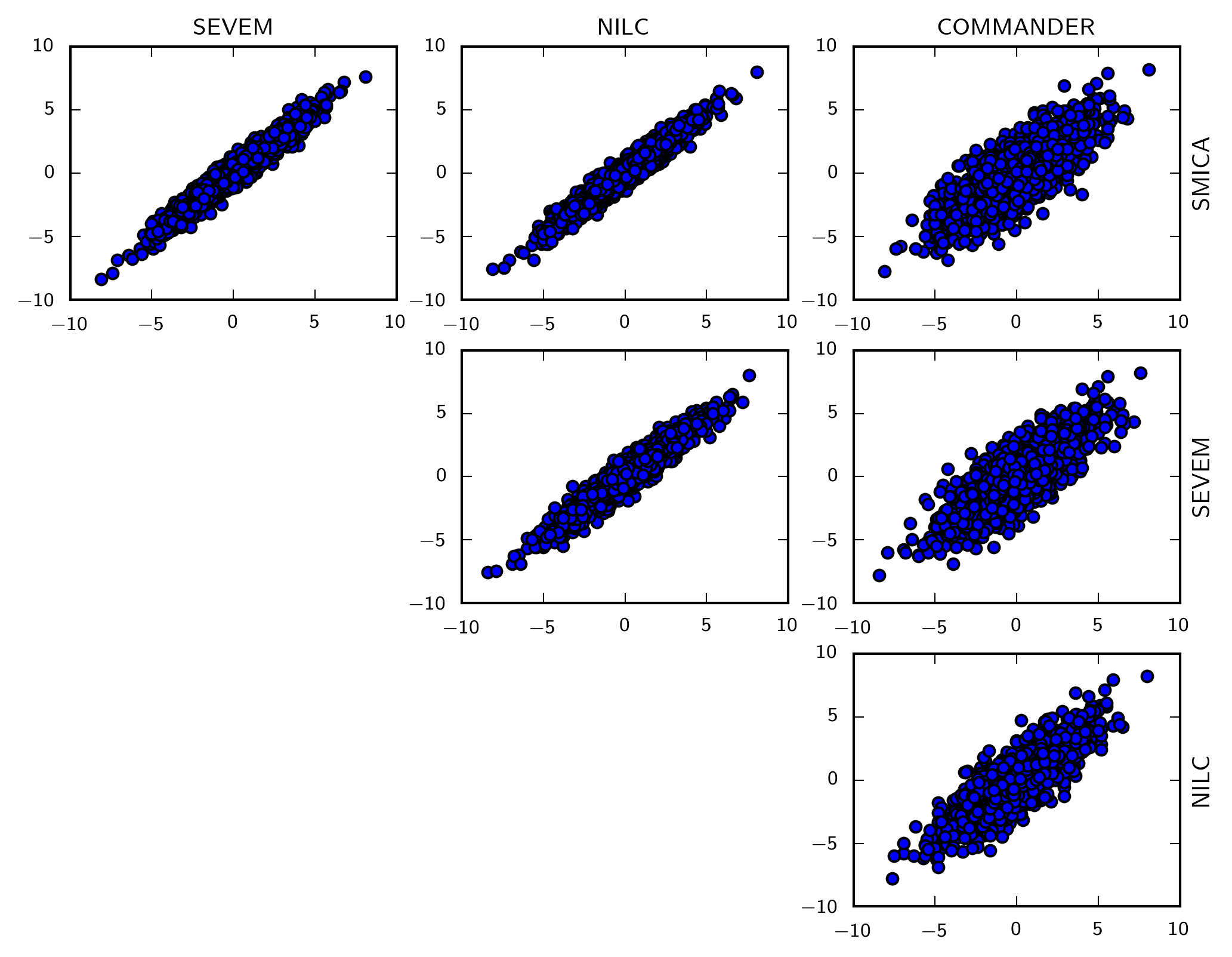
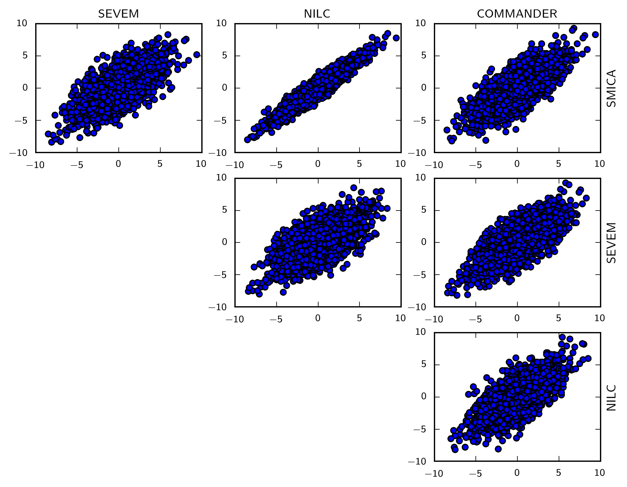
|
|
||||||||||||||||||||
7.2 Dependence on sky coverage
For each of the four component separation methods, we have used two different polarization masks, namely the same polarization mask as in Sect. 6, with (defined as the polarization “common mask” in Sect. 3.4), and an extended mask with . The temperature mask is kept unchanged in this test, and it covers a sky fraction (the temperature “common mask” of Sect. 3.4). We report the variation in for the three standard shapes in Table 13, which shows insensitivity to , in agreement with earlier results on T+E. In this case, however, the EEE results also seem quite stable, supporting the view that foreground residuals are not affecting our local, equilateral, and orthogonal results, especially for the final, combined T+E measurements. Tests on FFP8 simulations including foregrounds (see Sect. 7.3) suggest that measurements obtained from the SMICA and SEVEM maps are the most accurate under the current choice of mask. As a further check of these two methods we consider a third polarization mask, with , and repeat the combined T+E measurement, also finding stable results. For SMICA we find , , and , while for SEVEM we obtain , , .
We also perform model-independent checks by looking at the correlation coefficient between different sets of bispectrum modes, in a similar way to Sect. 7.1.2, but now changing the polarization mask. Results are reported in Table 16, and confirm that the data and simulations behave similarly, and that polarization modes display a lower correlation level than temperature.
|
||||||||||||||||||||||||||||||||||||||||||||||||||||||||||||||||||||||||||||||||||||||||||||||||||||||||||||||||||||||||||||||||||||||||||||||||||||||||||||||||||||||||||||||||||||||
|
||||||||||||||||||||||||||||||||||||||||||||||||||||||||||||||||||||||||||
7.3 Tests on simulations
We consider two realistic data simulations, one of which is Gaussian, while the other includes local NG. We start with a foreground-free realization, add foregrounds according to the Planck Sky Model, and finally process through the four component separation pipelines. By estimating in the input foreground-free simulation, for each method, and comparing to recovered from the cleaned maps (or with the input local , for the NG case), we can assess both the impact of foregrounds on our measurement before subtraction and which method gives the highest accuracy. The necessity to clean is very apparent in the middle set of columns in Table 17, where no cleaning has been performed.
SMICA and SEVEM give the best results, both in the G and NG tests. In the G test, reported in Table 17, SMICA results show an agreement between the input and the cleaned map at the level for all shapes, and for all of TTT, EEE, and T+E. SEVEM displays a similar level of accuracy, except for , where the difference is larger, but within one standard deviation. NILC and Commander clearly perform worse for the local shape, with NILC showing a 2 difference, and Commander even larger than that. In the NG test, reported in Table 18, SEVEM gives the most accurate results, recovering the input with accuracy or better. Results for SMICA are accurate at the 1 level for the TTT constraint, and worse (about 2 ) in EEE. However, the combined T+E measurement is again very good (). NILC is also performing very well in TTT and T+E, while the EEE result is more than 2 off.
The test described here has several limitations, the main and most obvious one being that it has been performed on just two maps (due to lack of availability of a large sample of this type of simulation at this stage). Another clear issue is that some methods, in particular Commander, seem to perform much better on actual data than on these simulations. On the other hand some important trends, observed in the data in previous tests, are clearly reproduced here, like the good stability of SMICA and SEVEM, especially for the combined T+E results and, most notably, the fact that the clear degradation in the accuracy of the EEE measurement for some methods does not seem to propagate to T+E.
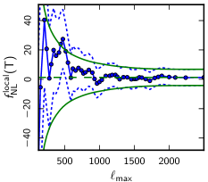
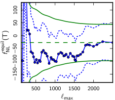
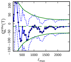
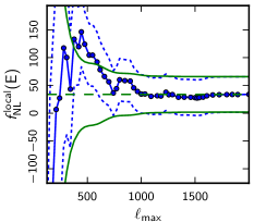
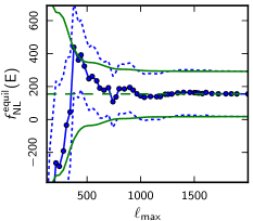
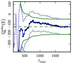
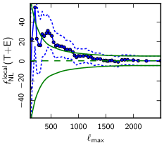
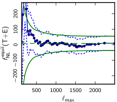
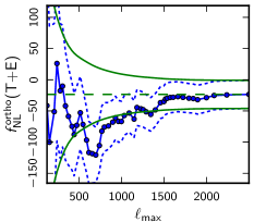
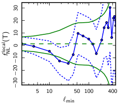
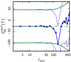
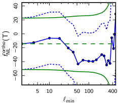
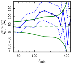
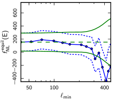
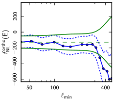
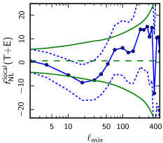
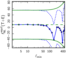
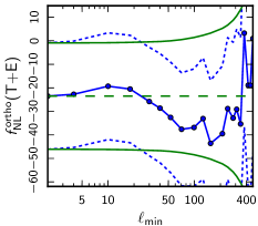
7.4 Dependence on multipole number
In this section we discuss another stability test of our results, namely the dependence of the results for on the maximum and minimum multipole number used in the analysis. This test is most easily performed with the binned bispectrum estimator, since it gets the dependence of on for free with its standard analysis, simply by leaving out bins in the final sum when computing (the binned equivalent of Eq. (41)).
The dependence on of the results for the three standard primordial shapes (local, equilateral, and orthogonal modes), is shown in Fig. 16, for T-only, E-only, and full T+E. As mentioned in Sect. 6, the KSW and binned estimators use for temperature, while the modal estimators use . As can be seen in the figure, both the T-only and T+E results are basically unchanged between and for all three shapes, showing that this difference has no impact on the results (as was to be expected from the excellent agreement between estimators in Table 10). In fact, the values of for T and T+E are reasonably stable (given their error bars) down to much lower values of , of about 1000.
On the polarization side we can draw a similar conclusion. The binned estimator uses for polarization, while the other estimators use , but we see that results for E remain basically unchanged between and . Central values and error bars for E for all three shapes have clearly converged by , and are in fact reasonably stable down to much lower values of about 700.
As we noted in the 2013 analysis (Planck Collaboration XXIV 2014), when going to the much lower WMAP resolution of , we agree with the slightly high value of that the WMAP team reported (Bennett et al. 2013). This value is also confirmed when including polarization. One can clearly see the value of the higher resolution of Planck.
The dependence on is shown in Fig. 17. Here all estimators used the same values, and . As explained in Planck Collaboration VII (2016), not all systematic and foreground uncertainties in the low- HFI polarization data have been fully characterized yet, and hence it was decided to filter out these data.
For equilateral and orthogonal shapes the values for and their error bars are quite stable as a function of up to about (and for E-only), which is not surprising, since these templates have little weight at low . The local template, on the other hand, depends very strongly on the lowest multipoles, which is reflected in the very rapid growth of the error bars when increases. Looking at T-only and T+E we see a very similar pattern, with being reasonably stable, although there are some jumps. The local result for E-only wanders a bit more outside of the region, in agreement with the other tests in this section, which also indicate that E-only is not as stable as T-only and T+E. However, that is still quite acceptable, given the small weight of E-only in the full T+E result.
One can work out quite generally that when is a subset of a data set , and and are the values of a parameter determined from these two data sets, then the variance of the difference is equal to Hence we can determine how likely the jumps in as a function of are. It turns out that the jump in the T-only value of between and is a effect (using the values of before subtraction of the ISW-lensing bias, which also depends on ). Similarly, the jump in the T-only value of between and is (by chance) also a effect. Given the fact that there are 57 bins, having such a jump appears to be consistent from a statistical point of view.
7.5 A directional analysis with a needlet-based modal estimator
The validation tests on simulations, described in Sect. 7.3, point to SMICA and SEVEM as the best foreground cleaning methods for estimation. Results in Table 10 show that SMICA also has slightly smaller error bars, thus making it the method of choice for our final results.
As a further check of residual foreground contamination in the SMICA map, in this section we investigate the possible directional dependence of SMICA-derived third-order statistics by means of a needlet-based modal estimator (i.e., an estimator based on the decomposition described in Sect. 3.2, and references therein, where we use cubic combinations of needlets as our basis modes). In other words, we analyse the behaviour of the needlet bispectrum (see Lan & Marinucci 2008, Rudjord et al. 2010 and Donzelli et al. 2012) on separate patches of the sky, and we study the fluctuations of the corresponding residuals.
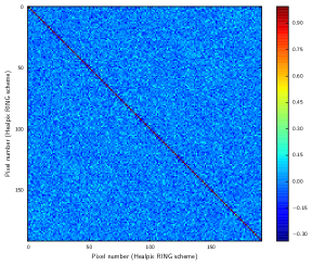
Rather than assuming a specific anisotropic model, we instead calculate the contribution to the local from different regions of the sky and look for evidence of anisotropy in the result.151515Even though we focus here on directional contributions to the local shape (which was typically found as one of the most sensitive to residual foreground contamination), this type of directional analysis can be done in a model-independent way, by looking separately at different needlet modes; we leave this for future work.
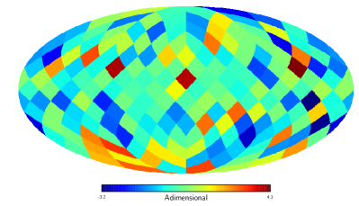
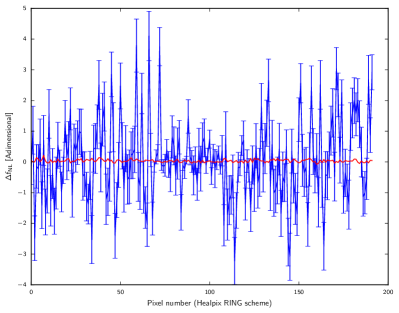
Our modal needlet estimator has been validated with respect to the procedures considered in Sect. 5, showing excellent agreement. Since in this paper we use the needlet estimator only in this section, and as a diagnostic tool, we will not explicitly report the outcome of these validation tests here, for the sake of conciseness. The advantages of using needlet-based modal estimators have been advocated in Lan & Marinucci (2008), Rudjord et al. (2010), Fergusson et al. (2010a), and Fergusson et al. (2012); we refer to these papers for more discussion and details. In short, however, they can be summarized as follows:
-
1.
it is possible to achieve a strong data compression, i.e., to investigate cubic statistics by means of a small number of modes (needlet frequencies) for many different bispectrum templates;
-
2.
needlet transforms have good correlation properties in pixel space, which allows study of the pixel contribution to the signal for the templates under investigation, by treating different directions independently.
In our analysis, we first divide the sky into several large “regions”, with boundaries defined by the pixels of a HEALPix grid (Górski et al. 2005). at lower resolution than the starting map (which is at ). For the low resolution grid we consider values between and . For each pixel in the coarse grid, we then compute the local using our modal needlet estimator, and neglect contributions from external regions.
The correlation matrices between measurements in different regions were computed via Monte Carlo simulations. was chosen, as providing the best tradeoff between having a large number of regions for directional analysis (i.e., the total number of pixels in the low resolution grid), and a low correlation between different regions. This is shown in Fig. 18. It is readily seen that, at , the correlation is largely concentrated in one or two points near the main diagonals (where it is still low, never exceeding ), and falls off rapidly for all other pixels. Note that the results here refer to temperature only. The EEE local polarization error bars are large, even for the full sky analysis, making this directional approach uninformative for Planck polarization data. We concentrate on the TTT bispectrum here, complementing other validation tests in this section, which are mostly focused on polarization.
Having obtained our correlation matrices, and having shown that different regions are essentially uncorrelated, we can then proceed to extract for each region in the actual SMICA map. As a test of directional-dependent contamination of the measurement, we can also compare our results, region by region, with the fluctuations expected by looking at the diagonal of our Monte Carlo correlation matrix.
The results of this analysis are shown in Fig. 19. In the left panel, we represent the directional local map, extracted with this method. In the right panel, we report the values, region by region, and compare them to expectations from simulations. The red line gives the expected standard deviation, while the blue one gives estimates on the component-separated maps with the Monte Carlo error bars. Our estimator is normalized in such a way that the sum of all these contributions would yield exactly the estimator for the full map, so these results can be viewed as a partition of the estimates along the different directions. It is readily seen that no significant fluctuation occurs, so that our results are consistent with the absence of directionally-dependent features (which could occur due to, for instance, residual foreground contamination). As an additional check, we have also investigated the possible presence of a dipole in these data, and found that our results are consistent with Gaussian isotropic simulations.
7.6 Summary of the main validation results
Throughout Sect. 7 we have shown a battery of tests aimed at evaluating the robustness of our data set, from the point of view of bispectrum estimators, focusing especially on the polarizaton part. We studied the stability of our results (local, equilateral, and orthogonal measurements, model-independent bispectrum reconstruction) under a change of sky coverage, multipole range, and choice of component separation methods. We also considered simulated data sets and studied the ability of different component separation methods to recover the input after foreground subtraction. Our main conclusions from these tests can be summarized as follows:
-
•
TTT and T+E results are stable both in the pixel and harmonic domains, for different component separation methods. For SMICA, we also checked that TTT temperature constraints on local show no evidence of a directional variation via a needlet-based analysis.
-
•
SMICA and SEVEM perform better than NILC and Commander at recovering the original in foreground-cleaned simulations. At the same time, SMICA allows slightly better constraints on than SEVEM, due to a lower (by a small amount) noise level.
-
•
EEE bispectra, and related measurements, have some problems, and do not pass all the tests. Different component separation methods show a low level of consistency (especially when comparing pixel-based cleaning methods to harmonic-based cleaning methods). This disagreement is only partly alleviated by choosing a larger E-mask, so that residual foregrounds do not seem to fully explain all issues. An important caveat, already pointed out previously, is that the noise model in polarized FFP8 simulations is known to underestimate the actual noise level in the data, leading to some degree of underestimation of the error bars in our EEE results. We stress again, however, that this has little impact on the final T+E constraints, due to the high noise level and consequent low statistical weight of EEE bispectra. This was verified in detail both on data and on simulations.
In light of the above analysis, we conclude that, as far as bispectrum estimation is concerned, our best cleaned map is the one produced by SMICA, in line with our previous analysis. We also conclude that our TTT-based constraints, summarized in Tables 10 and 11, are robust. Joint T+E constraints pass all our validation tests. On the other hand, in the light of the remaining issues in the EEE bispectra and in the FFP8 polarized simulations, as we stressed at the end of Sect. 6.1, we suggest that all measurements that include polarization data in this paper should be regarded as preliminary.
8 Other non-Gaussianity shapes for
| Independent Joint Shape . Cold dark matter Neutrino density Neutrino velocity Cold dark matter Neutrino density Neutrino velocity T a,aa. 1.3 5.4 1.3 5.4 1.3 5.4 21 13 27 52 32 48 T a,ai. 2 10 4 15 47 29 39 26 140 210 370 350 T a,ii. 59 910 130 280 750 360 17000 8200 4500 4500 1300 3800 T i,aa. 6 50 3.0 9.0 1.0 4.7 96 120 40 99 27 51 T i,ai. 3 66 5 22 26 21 2100 1000 220 630 75 170 T i,ii. 76 280 100 250 440 230 4200 2000 750 2400 970 1400 E a,aa. 34 34 34 34 34 34 66 50 51 120 140 150 E a,ai. 31 200 70 140 78 93 380 310 280 640 1100 620 E a,ii. 4200 4000 520 2300 190 940 8800 6100 6400 6200 9400 3900 E i,aa. 10 87 42 42 23 27 27 180 52 170 54 120 E i,ai. 94 250 83 130 45 62 910 770 670 850 190 420 E i,ii. 690 2200 390 1400 260 460 6000 5300 4100 5300 2200 1600 T+E a,aa. 0.7 4.9 0.7 4.9 0.7 4.9 5 10 35 27 2 24 T+E a,ai. 2.6 9.7 5 14 17 22 12 20 74 94 330 130 T+E a,ii. 130 450 130 240 130 230 1800 1300 3000 1400 3200 1200 T+E i,aa. 30 26 5.6 7.7 0.7 4.1 53 47 51 45 44 24 T+E i,ai. 26 38 2 19 6 15 140 170 170 210 20 74 T+E i,ii. 38 170 26 180 85 130 280 390 390 860 480 430 |
| Independent Joint Shape . Cold dark matter Neutrino density Neutrino velocity Cold dark matter Neutrino density Neutrino velocity T a,aa. 1.3 5.4 1.3 5.4 1.3 5.4 1.0 5.3 19 12 0.2 5.4 T i,ii. 76 280 100 250 440 230 65 280 840 540 440 230 E a,aa. 34 34 34 34 34 34 33 35 42 40 35 40 E i,ii. 690 2200 390 1400 260 460 210 2200 680 1700 31 540 T+E a,aa. 0.7 4.9 0.7 4.9 0.7 4.9 0.5 5.0 3.0 7.9 0.3 4.9 T+E i,ii. 38 170 26 180 85 130 35 170 120 290 87 130 |
This section discusses new searches for NG beyond standard single-field inflation. The focus here is on extensions to the analysis undertaken in Planck Collaboration XXIV (2014) with new limits on isocurvature models, further oscillatory models over a broader frequency range, and parity-violating tensor NG. However, we also briefly revisit all the non-standard models constrained in Planck Collaboration XXIV (2014), including effective field theory, non-Bunch Davies, and directionally-dependent models, in particular noting the impact of the new (preliminary) polarization data on the previous constraints.
8.1 Isocurvature non-Gaussianity
Here we show the results obtained for a study of the isocurvature NG in the Planck 2015 SMICA map using the binned bispectrum estimator. As explained in Sect. 2.3, we only investigate isocurvature NG of the local type, and in addition always consider only one isocurvature mode (either cold dark matter, neutrino density, or neutrino velocity isocurvature) in addition to the adiabatic mode. Note that the baryon isocurvature mode behaves identically to the cold dark matter one, only rescaled by factors of , so there is no need to consider it separately. In that case there are six different parameters: a purely adiabatic one (a,aa), which corresponds to the result from Sect. 6), a purely isocurvature one (i,ii); and four mixed ones (see Sect. 2.3 for an explanation of the notation).
The results are given in Table 19161616Compared to definitions in the literature based on and (see e.g., Langlois & van Tent 2012), here we adopt definitions based on and , in order to make the link with the standard adiabatic result more direct. Conversion factors to obtain results based on and are 6/5, 2/5, 2/15, 18/5, 6/5, and 2/5, for the six modes, respectively. and show no clear signs of any isocurvature NG. There are a few values that deviate from zero by up to about 2.5, but such a small deviation, in particular given the large number of results, cannot be considered a detection. We do see that many constraints are tightened considerably when including polarization, by up to the predicted factor of about six for the cold dark matter a,ii, i,ai, and i,ii modes in the joint analysis. As discussed in detail in Sect. 7, results including polarization data should be considered preliminary, and that is even more important here, since these results depend so strongly on the additional information from polarization.
In the results so far we allowed for a possible correlation between the isocurvature and adiabatic modes. However, if we assume that they are completely uncorrelated, with a zero cross power spectrum, then there are only two parameters, the a,aa and i,ii ones. In Table 20 we give the results for this uncorrelated case. The independent results are the same as in the previous table, while in the joint results one can clearly see the difference between the neutrino density mode (the bispectrum template of which has a large overlap with the adiabatic one), and the cold dark matter and neutrino velocity modes (with templates that are very different from the adiabatic one). Again there is no evidence for any isocurvature NG; the almost result for the neutrino velocity isocurvature mode in the temperature-only case does not survive the addition of polarization.
8.2 Feature models
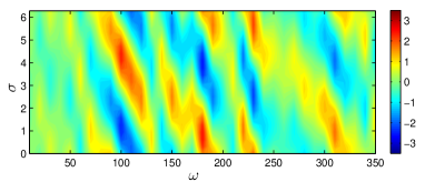
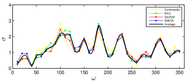
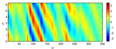
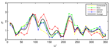


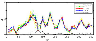
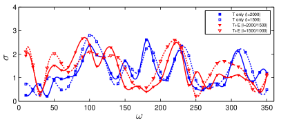
An important and well-motivated class of scale-dependent bispectra is the feature model, characterized by linear oscillations described by Eq. (15) and its variants in Eqs. (16) and (18). In Planck Collaboration XXIV (2014) we performed an initial search for a variety of feature models using the Modal estimator. This earlier search was limited to by the native resolution of our implementation of the Modal estimator (using 600 modes), roughly the same range as the initial WMAP bispectrum feature model searches at lower precision (with only eigenmodes (Fergusson et al. 2012). Note, in the previous Planck release we used wavenumber in line with the theory literature, but here we switch to frequency , in line with more recent observational power spectrum searches; the two are related by . With the improved estimator resolution (now using 2001 modes) we are able to achieve convergence over a broader range up to . We perform a frequency scan of 350 sampling points between and , i.e., 35 independent frequencies and 10 phases. We also extend the number and variety of feature and resonance models that are investigated, essentially probing the resolution domain in which we have obtained a reliable Modal bispectrum reconstruction (see Fig. 4).
Constant feature ansatz: For the constant feature shape of Eq. (15), we can extend the frequency range much further with another approach. As the bispectrum in Eq. (15) is separable, it allows the construction of a KSW estimator (Münchmeyer et al. 2014) for direct bispectrum estimation at any given frequency. The bispectrum can be written as a sum of sine and cosine components which can be estimated separately (equivalent to measuring the amplitude and phase above) and this method was used to constrain frequencies up to . The range where the two estimators overlap provides validation of the two methods and excellent agreement was seen (see Fig. 20).
Apart from cross-validation with two estimators, we have undertaken further tests to determine the robustness of the results to foreground and noise effects. In Fig. 21 (left panel), we show the effect on feature model results of the subtraction of the simple point source bispectrum, as well as the ISW-lensing bispectrum. This study was a major motivation for adopting the more conservative “extended” common mask, because the consistency between different component separation methods improved markedly for low frequencies, with the original common mask requiring much larger point-source subtractions (e.g., for NILC subtraction the maximum raw significance has reduced from to at ). After cleaning these signals, the SMICA, SEVEM and NILC results are in good agreement, and also consistent with each other when polarization is included (while the Commander results generally have a larger variance and so are not included in the plotted averages). Fortunately, the effect of subtracting ISW-lensing and point source bispectra diminishes rapidly at higher frequencies and should be negligible; subtraction was only undertaken in the Modal region . In Fig. 21 (right panel), we show the effect on the averaged significance of reducing the Planck domain from the usual to ( to for E-modes). Despite the non-trivial change in overall signal-to-noise entailed, there is no strong evidence for an -dependent signal, as might be expected if there was substantial NG feature contamination in the noise-dominated region. Finally, we note that most peaks at low show some correlation between T-only and T+E, although there are notable exceptions, such as the peak at , which is removed after inclusion of polarization (see also the phase plots in Fig. 20 before marginalization). The temperature feature peaks observed in Fig. 21 at , , and are consistent with the peaks identified previously in Planck Collaboration XXIV (2014).
In Fig. 20, the full set of frequency results, , for the constant feature model in Eq. (15) is shown for both the Modal and KSW estimators. There is good agreement for regions where the estimators overlap and PS and ISW lensing bispectra subtraction is not necessary (). Generally, there is tighter consistency between temperature-only results, than with polarization where there is additional scatter between foreground separation methods. Scanning across the full frequency range, there is no strong evidence for any large maximum that might indicate unequivocal evidence for a feature model signal. The maximum peak significance obtained with either T-only or T+E is consistent with expectations for a Gaussian model over this frequency range. In particular, for the KSW estimator using the SMICA data, the highest significance found in the range is 3.2 in T-only and 2.9 in . To gauge the likelihood of these results occurring randomly, realistic Gaussian SMICA simulations were analysed with the KSW estimator and found to typically produce a highest peak with over the same frequency range.
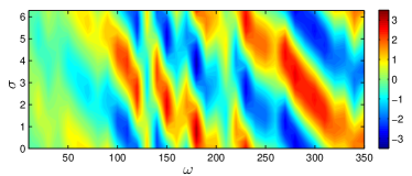
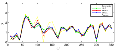
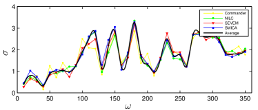
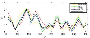
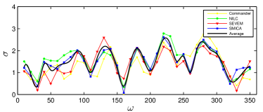
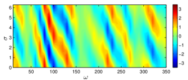
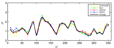
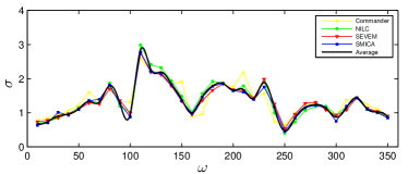
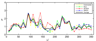
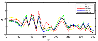
|
Generalized feature models: We have also deployed the Modal estimator to look at (non-separable) feature models with equilateral and flattened cross-sections, as motivated by varying sound speed scenarios and those with highly excited states, respectively. In the left panels in Fig. 22 we show results from the equilateral feature model of Eq. (16), including the frequency/phase contours before marginalization for the SMICA T-only map. Multiple peaks are apparent in the temperature signal across the Modal range up to an average maximum raw significance. However, from the lower panel it is clear that the polarization signal is not well correlated with the temperature in the equilateral case, generally reducing peak heights with the maximum now about (while eliminating the peak altogether). This temperature peak remains present with the cutoff, where the signal is slightly higher, but the polarization in this case is less well correlated (using ). For Gaussian noise we would not expect polarization to reinforce a high temperature signal on average. It may also be that the equilateral temperature signal has some residual diffuse point-source contamination. The equilateral feature model is the most affected by the removal of point sources, so the presence of a more complex correlated PS bispectrum (not removed by the constant PS template subtraction) remains for future investigation.
Results for the flattened feature model in Eq. (18) are shown in Fig. 22 (right panels), displaying more coherence between temperature and polarization. The temperature signal with a peak between is reinforced by polarization and merges to make a broad 3 peak around , together with another distinct peak at . Such broad frequency peaks are not expected, because neighbouring feature models should be nearly uncorrelated over a range (as we discuss below). As the phase plots in Fig. (22) indicate, this breadth in frequency may reflect the neighbouring feature models adjusting phase to match an underlying NG signal of a related, but different, nature. We note also that the frequency region for is susceptible to some degeneracy with cosmological parameters. We shall consider a “look-elsewhere” statistical analysis of these results below.
Single-field feature solutions: We have also searched for the specific analytic solutions predicted for single-field inflation models with step-like potential features, as given in Eqs. (19) and (20), with results shown in Fig. 23. The highest peaks for the -cosine model occur around with temperature-only, then rises to 2.7 when polarization data are included, again with peaks at other distinct frequencies apparent. The -sine model shows a similar apparent signal level, with a maximum T-only peak, dropping to with polarization. One further difficulty with a positive interpretation of these bispectrum results in this low frequency range is that stronger S/N counterparts in the power spectrum are predicted for these simple models (Adshead et al. 2011), whereas no significant correlated oscillation signals are apparent at the relevant peak frequencies Planck Collaboration XX (2016).
Feature model peak statistics: In order to determine consistency with Gaussianity for these feature model results, we can apply a number of statistical tests developed for this specific purpose (Fergusson et al. 2015) and, if warranted, also apply these jointly in combination with power spectrum results, as for the WMAP polyspectra analysis (Fergusson et al. 2014). When scanning across the parameter-dependent feature models, we are searching through independent models for which Gaussian noise, by chance, can lead to a large apparent signal. We must correct for this multiplicity of tests when determining the actual significance of results for a given model — this is a quantitative correction for any model with free parameters, distinct from the a posteriori choice of models to test. The simplest approach is to determine whether the maximum peak is consistent with Gaussian expectations, which can be determined from Monte Carlo simulations. However, in Fergusson et al. (2015) it was recognized that these feature models can be accurately characterized analytically with a -distribution having two degrees of freedom171717For the feature model with parameters , the adjusted significance for the raw significance after accounting for the “look-elsewhere” effect is given by (Fergusson et al. 2015) (71) where is the cumulative distribution function of the -distribution of degree two and is the effective number of independent feature models. This can also be used to investigate whether feature models are contributing at several frequencies. This multi-peak statistic integrates over all peak signals using the corrected significance , i.e., (72) where is the sampling step-size and is the effective correlation scale between independent models given by . Essentially this sums up all significant peaks that have a non-zero adjusted significance, after accounting for the look-elsewhere effect in Eq. (71).. Taking and using this analysis, the frequency step size between models that are uncorrelated is approximately , so we have an effective number of independent feature models for the Modal frequency range (with across the larger constant feature survey range). Accordingly appropriate look-elsewhere corrections have been applied to find an adjusted significance for the maximum peak signal found in all the feature model searches undertaken, which is shown in Table 21. Given that this feature model survey is over many independent frequency models and combinations of data, even the highest raw significances above (“Raw” column in Table 21) are reduced to a corrected significance below (“Single” column). Hence, there appears to be no evidence from maximum peak statistics for feature model deviations from Gaussianity.
Nevertheless, we also examine the possibility that multiple feature models are contributing to a NG signal, given the apparent emergence of several preferred frequency peaks. This integrated multi-peak statistic can also be accurately approximated analytically (Eq. 72) using a -distribution; essentially we sum over all independent frequencies using the single peak significance adjusted for the “look-elsewhere” effect (see Eq. (71)). Most of the signal surveys exhibit an unusual number of broad overlapping peaks within the accessible frequency domain, so the multi-peak statistic does yield a much higher significance, with many models above 2 after “look-elsewhere” correction. Notable cases are the temperature-only signal for the equilateral feature model which yields an average significance of across the foreground-cleaned maps with concordant bispectrum results (i.e., SMICA, SEVEM and NILC); however, this interesting multi-peak significance drops to only when the polarization data are included (assuming the reliability of results). On the other hand, the flattened feature model has an average multi-peak significance of in temperature only, which rises to with polarization included (higher at if Commander data were to be included in the average). In this case, beyond the number of peaks, it is also their width that contributes, with the main signal around , much broader than . Finally, after look-elsewhere effects are taken into account, the -cosine single-field solutions yield multi-peak statistics that rise with the inclusion of polarization data from to , while the -sine falls from () to ().
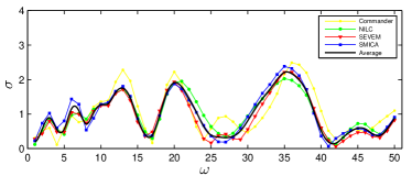
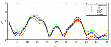
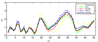
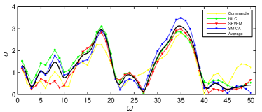
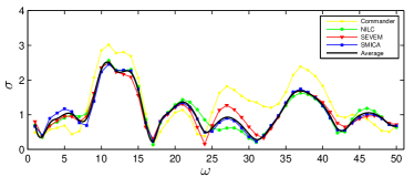
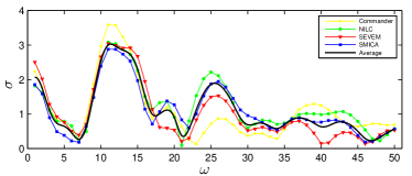
An interesting, but not entirely coherent, picture emerges from these searches for non-standard models in the new Planck temperature data, especially when combined with the additional (preliminary) polarization information. In Planck Collaboration XXIV (2014), we noted that the feature model searches provided interesting hints of NG. This more rigorous statistical analysis confirms this view, allowing for several alternative feature model explanations of the apparently high NG signal observed in the bispectrum reconstructions (see Fig. 4). However, there is no strong evidence for a single large feature model at a particular frequency; rather, the high multi-peak statistics indicate signal that is spread across several broad peaks. Given the variability between different feature models and polarization component-separation methods, we note the caveat that the integrated multi-peak statistic could be sensitive to calibration issues and foreground contamination. For this reason, we do not make strong claims for these non-standard signals at this stage, but we note that oscillatory models will continue to be investigated thoroughly over a wider frequency domain and using the more reliable polarization data available in the final Planck data release.
|
8.3 Resonance/axion monodromy models
Generalized resonance models: Using the Modal expansion, we have embarked on a survey of the simplest resonance model (Eq. 10), as well as the equilateral and flattened variants proposed in the literature, i.e., described by Eqs. (2.4) and (14), respectively. The raw significance for the resonance models for both temperature-only and temperature plus polarization data are shown in Fig. 24; these are the maximal results marginalized over the phase parameter . Previously, the resonance model was studied in Planck Collaboration XXIV (2014) using the Modal expansion over a narrower frequency range yielding no results above a raw significance of . In this extended analysis over a wider frequency range, the constant model (Eq. 10) produces peaks for T-only, and for T+E. The equilateral resonance model (Eq. 2.4) achieves a maximum in T-only at , rising to a more impressive average for T+E. For the flattened case (Eq. 14) we have and , respectively at . Qualitatively, the results shown in Fig. 24, exhibiting broad peaks, are similar to those for feature models.
Resonance model peak statistics: To determine the statistical significance of these results given the look-elsewhere effect of scanning across the parameters , we have used the two peak statistics defined above in Eqs. (71) and (72) for feature models (Fergusson et al. 2015). In this case, the maximum peak statistic for the constant resonance model of (T+E) is readjusted to an unremarkable “look-elsewhere” single peak significance of . Likewise the apparently significant results above for the equilateral and flattened models now fall below with T+E. Using the single peak statistic alone, we would conclude that there is no strong evidence for any individual resonance model. Resonance models also generate oscillations in the power spectrum, and an analysis based on the 2015 temperature and polarization likelihood is presented in (Planck Collaboration XX 2016). A combined statistical treatment of resonance model power spectrum and bispectrum results will be reported in the future.
The multi-peak statistic in Eq. (72) integrates the resonance model signal across all frequencies to determine consistency with Gaussianity. The constant resonance model has a modest multi-peak signal but, like the feature models, the equilateral and flattened resonance shapes offer stronger hints. The multi-peak equilateral signal rose from (T-only) to (T+E) after adjusting for the “look-elsewhere” effect, while the flattened signal went from (T-only) to (T+E). These interesting results, reflecting those obtained for feature models, suggests the fit to any underlying NG signal might await alternative, but related, oscillatory models for a more compelling explanation.
High frequency resonance model estimator: We have further surveyed the simple resonance model (Eq. 10) with a second approach. Using a model-specific expansion in terms of linear oscillation, proposed in Münchmeyer et al. (2015), it is possible to extend the frequency range of the analysis considerably. In this approach one exploits the fact that any bispectrum shape which is a function of can be expanded in Fourier modes of , resulting in an effectively one-dimensional expansion, as opposed to the general Modal expansion. In the present implementation we use 800 sine and cosine modes, which cover the full frequency space of the power spectrum search, i.e., . The significances found with this method are presented in Fig. 25. As was the case for the feature model, we find that SMICA, SEVEM and NILC results are in good agreement in both temperature and polarization, while Commander results generally have larger variance and so are not included in the plotted averages. We find that the largest peak of the average is in temperature and in temperature and polarization combined. The results of the Modal expansion discussed in the previous paragraph are in good agreement with the high frequency resonance model estimator in the overlapping frequency range.
Due to the high computational demands of this analysis, we have only exactly assessed the look-elsewhere effect for SMICA T data, for which we find an expected maximum peak of in the case of Gaussian maps, to be compared to in the SMICA T data, demonstrating that the results are fully consistent with Gaussianity. The expected maximum peak for Gaussian maps was calculated from the Fisher matrix with the method described in Meerburg et al. (2015). The average over component separation methods as well as the T+E data is even less significant. For the high frequency estimator we have assessed the significance of multiple peaks in the following way. Define the multi-peak amplitude as the sum of squares of the highest significances in the frequency range, i.e., , where only approximately independent peaks with are considered. One can then compare to its distribution in the Gaussian case and get an individual significance for each number of peaks , where we assume . The multi-peak statistic is then obtained by maximizing over , leading to an additional look-elsewhere effect that we also accounted for. In this way we find that in the SMICA T data the raw peak maximum , is reduced to for the single-peak statistic and to in the multi-peak case. This large reduction in significance is due to the large number of independent frequencies as well as to the maximization over phases. One may argue that the frequency range is too large, as EFT arguments for resonance non-Gaussianities (Behbahani et al. 2012) limit the frequency range to . As an example, we have therefore also calculated the look-elsewhere-corrected significances when we limit the analysis to . In this case we find a single-peak significance of and a multi-peak significance of . Clearly the results are fully consistent with Gaussianity.


|
8.4 Equilateral-type models and the effective field theory of inflation
There is considerable interest in equilateral-type models because they are physically well-motivated, through e.g., varying sound speed scenarios. There are generic predictions available from the effective field theory of inflation, notably the two specific effective field theory (EFT1 and EFT2) shapes that give rise to the equilateral and orthogonal approximations. These models were previously constrained in Planck Collaboration XXIV (2014) and the reader is referred to section 2 of that paper for analytic expressions for the specific shapes constrained here. In Table 23, we list the main equilateral-type models in the literature, giving constraints for T-only and T+E. All these models correlate well with the equilateral ansatz (Eq. 12) and likewise do not show a significant signal. However, despite this correlation, it is interesting to note the variation between models, largely due to the difference between these shapes in the flattened limit. The implications of these results are discussed in Sect. 11.
|
8.5 Models with excited initial states (non-Bunch-Davies vacua)
Non-Bunch-Davies (NBD) or excited initial states are models which produce flattened (or squeezed) bispectrum shapes. The wide variety of NBD models that have been proposed are briefly classified and labelled in Sect. 2, following a more extensive overview in section 2 of Planck Collaboration XXIV (2014) where more analytic forms and the first constraints were presented. The latest Planck constraints for these models are listed in Table 24, obtained using the Modal 2 estimator with polarization, Despite the apparent “flattened” signal seen in the Planck bispectrum reconstructions (Fig. 4), this is generally not matched well by the specific modulation induced by the acoustic peaks for these scale-invariant NBD models. Tight constraints emerge for most models. The largest signal obtained is from the NBD sinusoidal shape which gives a T-only raw significance, rising to for T+E; this is hardly an impressive correspondence given the number of models surveyed and the parameter freedom used in maximizing the signal. However, an important caveat for NBD models is that the predicted shapes can be very narrow in the flattened limit, in which case solutions have been smoothed to match the current Modal resolution (though this has improved considerably since the Planck 2013 NG analysis). An improved match to the warm inflation shape means that the final constraint shown in Table 24 is more robust, with further implications discussed in Sect. 11.
8.6 Direction-dependent primordial non-Gaussianity
We impose observational limits on direction-dependent primordial NG parametrized by Eq. 25. Rather than using and we instead choose to work with the non-linearity parameters and (chosen to match a primordial bispectrum that is equal to the equilateral shape in the equilateral limit) keeping the notation from the 2013 results. We estimated the values from temperature data and high-pass filtered polarization data from the four foreground-cleaned CMB maps SMICA, NILC, SEVEM, and Commander, where we apply the common mask. The details of the KSW estimator and its derivation is presented in Appendix A. For temperature data, we use the common mask as adopted in Planck Collaboration XII (2014), which has more conservative foreground masking than the newly available mask. We choose the more conservative foreground masking, considering the fact that anisotropic NG is more sensitive to residual foregrounds. We set the maximum multipole to 2000 and 1000 for temperature and polarization data, respectively. Validating our analysis pipeline with realistic simulations, we find that the asymmetry of the Planck beam, coupled with the Planck scanning pattern, inflates the statistical fluctuations of the significantly. Noting the large angular scale of artificial anisotropy produced by the beam asymmetry, we set the minimum multipole to 101, and find that the statistical fluctuation of estimation from simulated data is close to the theoretical expectations.
These two shapes are also constrained using the Modal 2 estimator, which is not affected by the beam asymmetry and is used in the same form as elsewhere in the paper with multipoles from to and to being used for temperature and polarization, respectively. The present constraints are consistent with those found for T-only in Planck Collaboration XXIV (2014), but at higher resolution convergence has improved considerably, reflected in the lower variance.
|
We find that the ISW-lensing bispectrum and the unresolved point-sources bispectrum bias the estimation of the , in particular in the analysis of temperature data. For our final values, we subtract both these biases from our estimation. In Table 25, we report the estimated value of from the foreground-cleaned CMB maps. For the effect of the differing -ranges between the two estimators is not so significant and the results are quite consistent. For , which has significant signal in the squeezed configuration, the effect of removing small scales from the KSW estimator is more pronounced, resulting in significantly enlarged error bars. In light of this, the differences seen between the central values for the two methods is to be expected and does not indicate any inconsistencies between the two approaches. The slight differences between the results from different foreground-cleaned temperature maps are within the likely range of statistical fluctuations, estimated from realistic simulations of CMB and noise propagated through the pipelines of foreground-cleaned map making. As seen in Table 25, we find that the estimated values of from Planck 2015 temperature plus polarization data are consistent with zero.
8.7 Parity-violating tensor non-Gaussianity
We present observational limits on the parity-violating tensor nonlinearity parameter from the temperature and -mode polarization data. Unlike the usual scalar-mode templates, the CMB bispectra sourced from the tensor NG (Eq. 29) are written in non-factorizable forms (Shiraishi et al. 2013b); hence, we use the separable Modal pipeline in our bispectrum estimations.
The parity-violating NG under examination induces non-vanishing signals not only in parity-even configurations () but also in the parity-odd ones () in the temperature and -mode polarization bispectra (Shiraishi et al. 2013b). The optimal estimator, including all (even + odd) bispectrum signals, is expressed by the linear combination of the parity-even and parity-odd estimators, reading (Liguori et al. 2015)
| (73) |
where is the normalization factor (related to the Fisher matrix as ) defined for . The parity-even estimator can be computed using the original Modal methodology (Fergusson et al. 2010a, 2012; Fergusson 2014; Liguori et al. 2015), while in computations of the parity-odd estimator , we follow the extended spin-weighted pipeline (Shiraishi et al. 2014, 2015; Liguori et al. 2015).
Our estimations (with both temperature and polarization data) are based on the resolution of and HEALPix , leading to feasible computational costs. This choice is not expected to change the results significantly, in comparison to the analysis at higher resolution, e.g., and Healpix , since the cosmic variance and instrumental noise are already far higher than the signals for (Shiraishi et al. 2013b). Only in the polarization data analysis is an effective also adopted, which is motivated by the high-pass filtering process for in component separation.
Within the above ranges, the theoretical bispectrum templates are decomposed with the eigenbasis composed of polynomials and some special functions reconstructing the tensor-mode features, e.g., temperature enhancement due to the ISW effect (), and two -mode peaks created by reionization () and recombination (). The resulting factorized templates are more than correlated with the original ones. The validity of our numerical computations has been confirmed through the map-by-map comparisons of at very low resolution, showing the consistency between the values from the Modal methodology and those obtained by the brute-force summations like Eq. (3). We have also checked that our parity-even estimator successfully leads to the constraints on , , and at , compatible with the results from the binned estimator.
Our limits estimated from the foreground-cleaned temperature and high-pass filtered polarization data (SMICA, SEVEM, and NILC) are summarized in Table 26. The data and MC simulations used here, including all experimental features, i.e., beam, anisotropic noise levels and partial sky mask, have been inpainted using the identical recursive process adopted in the standard estimations (see Sect. 3.5). The sky fractions of the temperature and polarization masks adopted here are, respectively, and . Although the error bars and the linear terms have been computed using 160 MC simulations, the resulting error bars are close to the expected values, .
We have confirmed the stability of the T-only constraints, and significant scatter of the E-only constraints both in the parity-even case and in the parity-odd one, when changing . Such -mode instability has given insignificant effects on our T+E constraints in the parity-even case, as they are determined almost exclusively by TTT, like the scalar NG analyses. In contrast, our parity-odd T+E results vary a lot, due to the -mode scatter (quantitatively speaking, only a few percent change of has shifted by more than ), because TTE and TEE contribute significantly to the signal-to-noise ratio in the parity-odd case (Shiraishi et al. 2013b). Table 27 presents the correlations of the bispectra reconstructed from the component separated maps, also indicating the robustness of the T-only constraints and the instability of the E-only results. We report only stable results in Table 26 and conclude that there is no evidence at of in the parity-even, parity-odd or their whole domain.
The parity-odd components of the TTT and EEE bispectra extracted model-independently from the SMICA data are visually represented in Fig. 26. It is apparent from this figure that the Planck TTT bispectrum has similar features to the WMAP one (Shiraishi et al. 2015), e.g., distinctive signals distributed around . As indicated by the roughly correlation between the SMICA and WMAP bispectra (see Table 27), the Planck T-only limits in Table 26 are close to the WMAP ones (68 % CL): for parity-even; and for parity-odd (Shiraishi et al. 2015).
| . Even Odd All SMICA T. 2 15 120 110 4 15 T+E . 0 13 SEVEM T. 2 15 120 110 5 15 T+E . 4 13 NILC T. 3 15 110 100 5 15 T+E . 1 13 |
|
||||||||||||||||||||||||||||||||
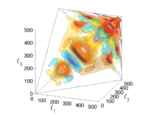
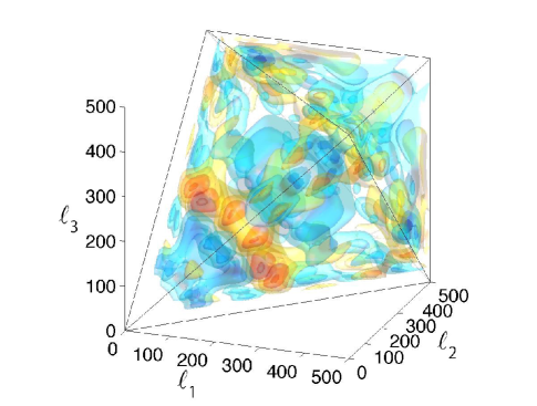
9 Limits on the primordial trispectrum
So far, we have considered a variety of physically motivated possibilities for the inflationary 3-point function, or bispectrum. A similar phenomenology exists for the 4-point function, or trispectrum. Our constraints on the trispectrum will use CMB temperature only; we do not use polarization in this section. We start by briefly reviewing the inflationary physics and classifying the signals we will search for.
First, some notation: a “primed” -trispectrum denotes the connected trispectrum without its momentum-conserving delta function, i.e.,
| (74) |
where “+ disc.” denotes the disconnected contributions to the 4-point function.
One possible signal is the “local” trispectrum , which arises if the non-Gaussian adiabatic curvature is of cubic-type form (see, e.g., Okamoto & Hu (2002)), i.e.,
| (75) |
where is a free parameter and is a Gaussian field. In this model, the bispectrum is zero (since there is a symmetry) and the trispectrum is given by
| (76) |
Analogously to the case of the local bispectrum, , the observational signal-to-noise for is largest in the “squeezed” limit, , and there is a consistency relation which shows that in single-field inflation, the four-point function is always small in the squeezed limit (e.g., Senatore & Zaldarriaga 2012a). Thus can only be detectably large in multi-field models. Conversely, there are multi-field models where is detectable. The main obstacle here is technical naturalness, i.e., ensuring that radiative corrections do not generate an observationally larger bispectrum. This can be the case if a large bispectrum is forbidden by a symmetry, or by supersymmetry (Senatore & Zaldarriaga 2012b).
A further category of four-point signals can be obtained by adding quartic interactions to the inflationary action. Following Smith et al. (2015), we will concentrate on the simplest possibility, by considering quartic operators consistent with the symmetries of inflation and having the lowest possible number of derivatives (Bartolo et al. 2010b; Senatore & Zaldarriaga 2011, 2012b). There are three such operators, of the schematic form , , and . By a short calculation using the in-in formalism (Maldacena 2003), the associated four-point functions are (Smith et al. 2015; see also Huang & Shiu 2006):
| (77) | |||||
| (78) | |||||
| (79) | |||||
Here and we have introduced parameters , , and to parametrize the amplitude of each trispectrum.
The normalization of the -parameters is chosen so that for “tetrahedral” configurations, with and . This is the analogue of the commonly-used normalization for the bispectrum, where parameters are defined so that for equilateral configurations with .
For simplicity in Eqs. (77)–(79) we have assumed a scale-invariant initial power spectrum . In order to analyse Planck data, we must slightly generalize this to a power-law spectrum . Our scheme for doing this follows Appendix C of Smith et al. (2015).
A Fisher matrix analysis shows that there is one large correlation among the three trispectra in Eqs. (77)–(79), so that to an excellent approximation we can treat only two of the trispectra as independent. To quantify this, in Smith et al. (2015) it is shown that the shape is correlated to a linear combination of the shapes and . Therefore, we will only search for the parameters and .
We note that the analysis that leads to the trispectrum shapes and is very similar to the analysis that leads to the “standard” bispectrum shapes and . However, there are some minor differences as follows. In the bispectrum case, one considers the cubic operators and , but it is conventional to define observables which are related to the operator coefficients by a linear transformation. This is done because the two cubic operators are about correlated, so it is convenient to orthogonalize. In the trispectrum case the correlation is smaller (around for Planck), and we have chosen to omit the orthogonalization step. Another reason to omit the orthogonalization step is that the trispectrum shape is a signature of multi-field inflation. In single field inflation, the trispectrum is not technically natural; radiative corrections generate cubic operators of the form or , which generate a bispectrum with larger signal-to-noise.
There are more trispectrum shapes one might consider. For example, classifying Galilean invariant quartic operators leads to higher-derivative trispectra, which are not highly correlated to the trispectra considered above (Bartolo et al. 2013; Arroja et al. 2013). We have only considered “contact” diagrams arising from one power of a quartic operator, and it would be interesting to study “exchange” diagrams arising from two cubic operators and exchange of a light particle (e.g., Chen et al. 2009; Arroja et al. 2009; Chen & Wang 2010; Bartolo et al. 2010a; Baumann & Green 2012). We leave these as extensions for future work.
Summarizing, we will search for the following trispectrum signals:
| (80) |
9.1 Data analysis
Turning now to data analysis, we use the machinery from Smith et al. (2015). The first step is to represent each trispectrum as a small sum of factorizable terms as follows. The angular CMB trispectrum can be written either as an integral over comoving distance (in the case of ) or as a double integral over where is conformal time during inflation (in the case of the or trispectra). We approximate the integral by a finite sum, which represents the CMB trispectrum as a sum of terms that are factorizable in a sense defined in Smith et al. (2015). A large number of sampling points are needed to obtain a good approximation to the integral, leading to a large number of terms in the factorizable representation. However, there exists an optimization algorithm, which takes as input a trispectrum that has been represented as a sum of many factorizable terms, and outputs a representation with fewer terms. The reduction can be quite dramatic, as shown in Table 28. The optimization algorithm guarantees that the output trispectrum accurately approximates the input trispectrum, in the sense that the two are nearly observationally indistinguishable.
|
Armed with “small” factorizable representations for each trispectrum, the next step is to run an analysis pipeline that estimates the amplitude of each trispectrum from Planck data. We use the “pure MC” pipeline from Smith et al. (2015), which compares the trispectrum of the data to the mean trispectrum of an ensemble of simulations. This pipeline requires a filtering operation which processes the pixel-space CMB data and generates a harmonic-space map . Our filtering operation is defined by the following steps:
-
1.
Starting from the data , we compute (with uniform pixel weighting) a best-fit monopole and dipole outside the Galactic mask. We use the temperature “common mask”, the union of the confidence masks for the SMICA, SEVEM, NILC, and Commander component separation methods (Planck Collaboration IX 2016).
-
2.
The mask defines a few “islands”, i.e., isolated groups of pixels that are unmasked, but contained in a larger masked region. We slightly enlarge the mask so that it removes the islands.
-
3.
We classify the components of the masked part of the sky into “small” masked regions with pixels (at HEALPix resolution ), and “large” regions with pixels. Small regions usually correspond to point sources, and large regions typically correspond to areas of diffuse galactic emission. In small regions, we inpaint the CMB by assigning the unique map that agrees with the data on boundary pixels, and whose value in each interior pixel is the average of the neighboring pixels.
-
4.
In large regions, we do not inpaint the CMB, but rather apodize the boundary of the large region using cosine apodization with 12’ radius.
-
5.
We apply a spherical harmonic transform to the inpainted, apodized CMB map to obtain a harmonic-space map with . We then take the final filtered map to be
(81) where is the beam, is the fiducial CMB power spectrum, and is the sky-averaged noise power spectrum (without beam deconvolution). To motivate this choice of -weighting, we note that for an ideal all-sky experiment with isotropic noise, we have where are signal and noise realizations. In this case, Eq. (81) weights the signal as , which is optimal.
In our pipeline, we apply this filter to the component-separated SMICA maps (Planck Collaboration IX 2016), obtaining a harmonic-space map . We apply the same filter to 1000 Monte Carlo simulations to obtain an ensemble of harmonic-space maps. Our pipeline has the property that it always estimates the trispectrum of the data in excess of the trispectrum in the simulations. Since the simulations include lensing, this means that lensing bias will automatically be subtracted from our estimates.
Now that the filter, data realization, and Monte Carlo simulations have been fully specified, the details of the pipeline are described in section IX.B of Smith et al. (2015). For each trispectrum, the pipeline outputs an estimate of and an estimate of the statistical error. Our basic results are:
| (82) | |||||
No deviation from Gaussian statistics is seen. These results significantly improve the previous best constraints on the trispectrum from WMAP (Vielva & Sanz 2010; Smidt et al. 2010; Fergusson et al. 2010b; Hikage & Matsubara 2012; Sekiguchi & Sugiyama 2013; Regan et al. 2013; Smith et al. 2015) and large-scale structure (Desjacques & Seljak 2010; Giannantonio et al. 2014; Leistedt et al. 2014).
A constraint on from Planck 2013 data was recently reported by Feng et al. (2015), who find . Our central value in Eq. (82) agrees well with this result, but the statistical error is smaller by a factor of 2.3. This improvement is partly due to the lower noise levels in Planck 2015 data, and partly due to the use of a better estimator.
Each line in Eq. (82) is a “single-” constraint; i.e., the constraint on one parameter with the other -parameters held fixed. For joint constraints, one needs to know the full covariance matrix. The correlation between and the other two parameters is negligble, and the - correlation is:
| (83) |
multi-field models of inflation will generally give a linear combination of , , and trispectra. In this case we proceed as follows. First, if the coefficient is non-zero, we can use the near-degeneracy with a linear combination of the other two operators to absorb it into the effective values of and . A Fisher matrix analysis shows that the coefficients of this linear combination are
| (84) |
It is convenient to define the two-component parameter vector:
| (85) |
We also compute a two-by-two Fisher matrix , whose diagonal is given by , where is the single- statistical error in Eq. (82), and whose off-diagonal is , where is the correlation in Eq. (83). This procedure gives:
| (86) |
For a given parameter vector , we can define a trispectrum- by
| (87) |
where is the vector of best-fit single- values from Eq. (82). This definition of follows from the observation that is an estimator with expectation value and covariance matrix .
The inflationary implications of these trispectrum constraints are discussed in Sect. 11.5 below.
10 Minkowski functionals results
In this section, we present constraints on local NG at first and second order ( and ) obtained with Minkowski functionals (MFs) on temperature and polarization maps. MFs (Mecke et al. 1994; Schmalzing & Buchert 1997; Schmalzing & Gorski 1998; Winitzki & Kosowsky 1998) are a measure of fields’ local morphology used to constrain their stationarity, isotropy and Gaussianity. Mostly probing general NG in a frequentist fashion in two-dimensions on CMB maps (Eriksen et al. 2004; Komatsu et al. 2005; Modest et al. 2013; Natoli et al. 2010; Curto et al. 2008) or three-dimensions on LSS data (Park et al. 2005; Wiegand et al. 2014), they have also been used to measure specific NG targets with Bayesian methods, such as (Hikage et al. 2006, 2008; Ducout et al. 2013; Planck Collaboration XXIV 2014), other bispectrum and trispectrum shapes (Hikage & Matsubara 2012) and topological defects (Planck Collaboration XXV 2014). New developments have been made recently, using needlets (Fantaye et al. 2015), neural networks (Novaes et al. 2014) or allowing scale-dependent measurements (Munshi et al. 2013).
MF-based limits are well known to be suboptimal for and , but they provide an independent cross-check of bispectrum and trispectrum-based estimators. They are complementary to optimal estimators: they are weighted integrals of the polyspectra and are sensitive to any source of NG, including foregrounds and secondaries. While MFs are not always able to distinguish between these different sources and systematics, they allow upper bounds to be put on them.
The most recent constraints () from MFs on and have been obtained with WMAP (Hikage & Matsubara 2012) and Planck (Planck Collaboration XXIV 2014):
| (88) |
10.1 Method and definition of MFs
For a smoothed two-dimensional field of zero mean and of variance , defined on the sphere, we consider an excursion set of height , i.e., the set of points where the field exceeds the threshold . We use four functionals denoted by . The first three correspond to MFs: is the fractional Area of the regions above the threshold, is the Perimeter of these regions and is the Genus, defined as the total number of connected components of the excursion above the threshold minus the total number of connected components under the threshold. The fourth, , is the Number of clusters (also referred to as Nclusters). This is the number of connected regions above the threshold for positive thresholds and below the threshold for negative thresholds. Precise definitions and formulae for the quantities as well as their expectation values for Gaussian fields are summarized in Appendix B.
We calculate the four normalized181818Raw Minkowski functionals depend on the Gaussian part of fields through a normalization factor , a function only of the shape of the power spectrum. We therefore normalize functionals to focus on NG, see Appendix B. functionals on thresholds , between and .
For this analysis, we used the same temperature and polarization data, simulations and masks described in Sect. 3.4 for consistency with the bispectrum estimators. In addition, the maps are filtered to optimize constraints on local NG (Ducout et al. 2013), the filters used being similar to Wiener filters for and (), and for the first () and second () derivatives of these fields (Fig. 27):
| (89) | |||||
| (90) |
For the temperature map, known point sources in the mask are inpainted.
We define the vector as any combination with , , , being the vector measured on the data.
From these measurements, we then use a Bayesian method to jointly estimate and ,
| (91) |
We take a uniform prior for in the range to 400, and for in the range to , while the evidence is just considered as a normalization.
Assuming MFs are multi-variate Gaussian-distributed we obtain the posterior distribution for with a test
| (92) |
with
| (93) |
For this test, we use two types of simulations to first construct a model including primordial NG and secondly a covariance matrix
| (94) |
with averaged over the simulations. We now describe the details of these simulations.
-
•
Simulations 1: Non-Gaussian model
For the first type of simulation, we included all possible sources of NG, assuming that the total and individual levels of NG are small enough that MFs are linear with respect to those NG levels (Ducout et al. 2013). The three kinds of NG we included are foreground residuals (Galactic residuals with scalable amplitude , as well as radio sources, CIB anisotropies, secondaries (SZ, lensing and ISW-lensing, but not SZ-lensing) and primordial NG (, ):(95) We tried to reproduce all instrumental effects, with realistic effective beams (isotropic window functions), noise from FFP8 simulations (Planck Collaboration XII 2016), filtered with component separation weights. We checked the accuracy of these simulations by comparing them to FFP8 simulations, using no foreground and no primordial NG. The astrophysical models are provided by the Planck Sky Model (PSM, Delabrouille et al. 2013), while the primordial NG simulations are computed as in Elsner & Wandelt (2009). The lensing uses LensPix191919http://cosmologist.info/lenspix. The power spectrum used for these NG simulations and the lensing is the best-fit power spectrum from Planck 2013+ACT/SPT+BAO (Planck Collaboration XXII 2014). We created simulations , using maps for the primordial NG, while we had only one astrophysical foreground simulation.
-
•
Simulations 2: FFP8 (Planck Collaboration XII 2016) MC simulations
Since NG is weak, the covariance matrix is computed with simulations, including no primordial NG and no foregrounds. These simulations reproduce realistic instrumental effects (anisotropy of beams in particular), realistic noise and component separation filtering. The only NG still present in these simulations are lensing and the ISW-lensing correlation.
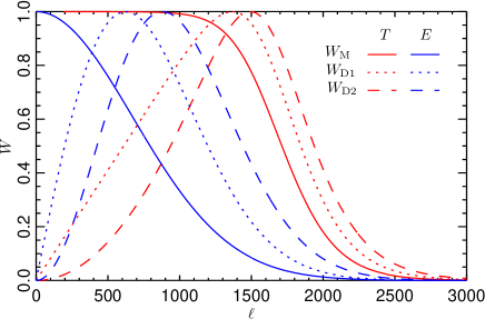
Validation of the estimator
Part of the validation for the MFs estimator is described in Sect. 5.3 for , to compare the results to bispectrum estimators on realistic simulations (FFP8 MC, second item above). In addition we present in Table 29 the results obtained on the same realistic simulations for , and on simulations containing primordial NG (first item above), with and , with 200 simulations used in each case. These tests have been performed using the SMICA method with lensing bias removed.
|
10.2 Results
Results for and estimation with MFs on the four component separated maps in temperature and polarization are presented in Table 30. The results for polarization -only maps are not quoted, since these results were not sufficiently stable (cf. Sect. 7.6). No deviation from Gaussianity is detected. T+E analysis generally finds higher values for , but remains consistent with Gaussianity.
The posteriors for and from SMICA are shown in Fig. 28. One interesting point is that the estimates of and are almost uncorrelated (); this can be inferred when we consider the parity of MF deviations from Gaussianity, which is different for the two parameters (Matsubara 2010).
Foreground and secondary biases are removed from these estimates, since the NG model directly includes them. However, an estimation of their contribution in the map is reported in Table 31.
|
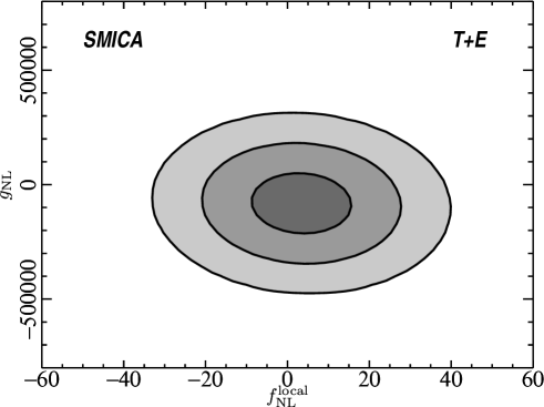
Foreground and secondary biases
Foreground residuals are generally negligible, in particular in the analysis. This is different from the Planck 2013 results, where the residuals were more important; this can be explained by the beam correction applied to these previous estimates which exaggerated signals from small scales.
Lensing has a significant signature in MF estimation of , but is even stronger in (the four-point correlation signature) and could be detected (and not treated just as a bias) with this estimator. The Wiener filters enhance the scales where lensing is dominant.
|
||||||||||||||||||||||||||||||||||||||||||
11 Implications for early Universe physics
The NG constraints obtained in this paper show consistency of Planck data with Gaussian primordial fluctuations, thus confirming the results obtained in the 2013 release (Planck Collaboration XXIV 2014) and improving them through the inclusion of CMB polarization data. The standard single-field slow-roll models of inflation have therefore been confirmed as a viable scenario for inflation, passing one of their most stringent tests, based on lack of measurable deviations from Gaussianity. The constraints obtained on local, equilateral, and orthogonal NG, after accounting for various contaminants, strongly limit different mechanisms proposed as alternatives to the standard inflationary models to explain the seeds of cosmological perturbations. Measurements on deviations from Gaussianity for other primordial bispectral shapes help to shed light on more subtle effects about the detailed physics of inflation.
As in Planck Collaboration XXIV (2014), in the following we derive limits on parameters of the models from the NG constraints in the following way (unless explicitly stated otherwise): we construct a posterior based on the assumption that the sampling distribution is Gaussian (as supported by Gaussian simulations); the likelihood is approximated by the sampling distribution, but centred on the NG estimate (see Elsner & Wandelt 2009); we employ uniform or Jeffreys’ priors, over intervals of the parameters values that are physically meaningful, or as otherwise stated; and in the cases when two or more parameters are involved, we marginalize the posterior to provide one-dimensional constraints on the parameter considered.
11.1 General single-field models of inflation
DBI models: DBI models of inflation (Silverstein & Tong 2004; Alishahiha et al. 2004), characterized by a non-standard kinetic term of the inflaton field, predict a non-linearity parameter , where is the sound speed of the inflaton perturbations (Silverstein & Tong 2004; Alishahiha et al. 2004; Chen et al. 2007b). The corresponding bispectrum shape is very close to the equilateral shape. Nonetheless we have constrained the exact theoretical (non-separable) shape (see equation 7 of Planck Collaboration XXIV 2014). The constraint we obtain from temperature data ( from temperature and polarization) at CL (with ISW-lensing and point sources subtracted, see Table 23) implies
| (96) |
and
| (97) |
In Planck Collaboration XXIV (2014) we constrained the so-called infrared (IR) DBI models (Chen 2005b, a), which arise in string frameworks. We focused on a minimal setup, considering a regime where stringy effects are negligible and predictions for primordial perturbations are built within standard field theory. In the companion paper Planck Collaboration XX (2016) we present an analysis of a more general class of IR DBI models which accounts for stringy signatures (see Bean et al. 2008) by combining Planck power spectrum and bispectrum constraints.
Implications for effective field theory of Inflation: In this subsection we use the effective field theory approach to inflation in order to translate the contraints on and into limits on the parameters of the Lagrangian of general single-field models of inflation (of the type models). In particular we derive the most conservative bound on the sound speed of the inflaton perturbations for this class of models.
The effective field theory approach (Cheung et al. 2008; Weinberg 2008) provides an efficient way to constrain inflationary perturbations for various classes of models that incorporate deviations from the standard single-field slow-roll scenario. In this approach the Lagrangian of the system is expanded into the (lowest dimension) operators obeying the underlying symmetries. We consider general single-field models described by the following action
where the curvature perturbation is related to the scalar field as . The inflaton interaction terms and generate two kind of bispectra with amplitudes, respectively, and , where is the amplitude of the operator (Senatore et al. 2010, see also Chen et al. 2007b; Chen 2010b). These two bispectra both peak for equilateral triangles in Fourier space. Nevertheless, they are sufficiently different, and the total NG signal turns out to be a linear combination of the two, leading also to an orthogonal shape. We can put constraints on and the dimensionless parameter (Senatore et al. 2010). Notice that DBI inflationary models corresponds to having , while and (or represent the non-interacting (vanishing NG) case.
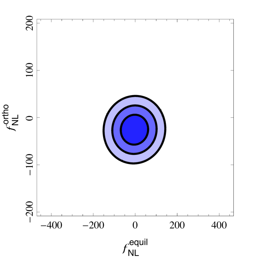
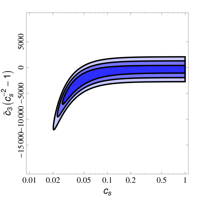
The mean values of the estimators for and are expressed in terms of and by
| (99) |
Here the coefficients come from the Fisher matrix between the equilateral and orthogonal templates and the theoretical bispectra predicted by the two operators and . We use a statistic given by , where (={equilateral, orthogonal}), being the joint estimates of equilateral and orthogonal (see Table 11), the covariance matrix of the joint estimators, and is provided by Eq. (11.1). As an example in Fig. 29 we show the , and confidence regions for and obtained from the constraints, requiring , and respectively (corresponding to a variable with two degrees of freedom). In Fig. 30 we show the corresponding confidence regions in the parameter space. Marginalizing over we find
| (100) |
and
| (101) |
The constraints improve by a few percent in T-only and by up to by including polarization, in comparison with those of Planck Collaboration XXIV (2014).
Galileon models of inflation: Galileon models of inflation (Burrage et al. 2011; Kobayashi et al. 2010; Mizuno & Koyama 2010; Ohashi & Tsujikawa 2012) are well motivated models based on the so called “Galilean symmetry” (Nicolis et al. 2009). They are characterized by stability properties that are quite well understood (ghost-free, and stable against quantum corrections) and can arise naturally within fundamental physics models (de Rham & Gabadadze 2010b, a). Moreover they are an interesting example of models where gravity is modified on large scales and we focus on them also as a typical example of a more general class of modified gravity theories that are ghost-free (the so called Horndeski theories, Horndeski 1974; see also Planck Collaboration XIV (2016) where these models are discussed in the context of dark energy/modifed gravity scenarios for the late time evolution of the universe). The predictions for the primordial perturbations are very rich. Bispectra can be generated with the same shapes as the “EFT1” and “EFT2” bispectra (see also discussion in Creminelli et al. 2011), however the amplitude(s) scale with the fluctuation sound speed as , differently from the general single-field models of inflation considered in the above subsection. They can be written as (at the lowest-order in slow-roll parameters)
| (102) | |||||
| (103) | |||||
Here , , and are dimensionless parameters of the models. In particular is the sound speed of the Galileon scalar field, while is a parameter that appears to break the standard consistency relation for the tensor-to-scalar perturbation ratio (, being the tensor spectral index)202020For the explicit expressions of these parameters in terms of the coefficients of the Galileon Lagrangian see Planck Collaboration XX (2016).. Accordingly to Eq. (11.1) a linear combination of these two bispectra generate equilateral and orthogonal bispectra templates212121 We note that we are neglecting corrections (where means also ); see (Burrage et al. 2011) and (Ribeiro & Seery 2011). These corrections will have a different shape associated with them and they are not necessarily small when compared with some of the terms displayed, e.g., the terms . . From the Planck constraints on and (see Table 11), we derive constraints on these model parameters following the procedure described at the beginning of this section. We choose log-constant priors in the ranges , and , together with a uniform prior . These priors have been choosen essentially on the basis of perturbative regime validity of the theory and to allow for a quite wide range of parameter values. In Fig. 31, as an example, probability contours are shown in the parameter space from the constraints, after marginalizing over the parameter . Marginalizing over both and we find
| (104) |
and
| (105) |
Notice that interestingly enough the parameter can be negative in principle, corresponding to a blue spectral tilt of inflationary gravitational waves (without any kind of instability). We therefore also explore this branch, with a log-constant prior (for ), , and the same priors for the other parameters as above. Fig. 32 shows the probability contours in the plane, after marginalizing over the parameter , for the branch. Marginalizing over both and gives
| (106) |
and
| (107) |
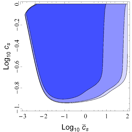
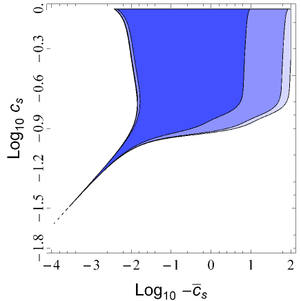
A combined analysis of the Planck bispectrum and power spectrum constraints on the Galileon models is presented in the companion Planck paper on inflation (Planck Collaboration XX 2016).
11.2 Multi-field models
Curvaton models: The simplest adiabatic curvaton models predict local NG with an amplitude (Bartolo et al. 2004c, b)
| (108) |
for a quadratic potential of the curvaton field (Lyth & Wands 2002; Lyth et al. 2003; Lyth & Rodriguez 2005; Malik & Lyth 2006; Sasaki et al. 2006), where is the “curvaton decay fraction” at the time of the curvaton decay in the sudden decay approximation. Assuming a uniform prior, , our constraint at 68 % CL (see Table 11) yields
| (109) |
while accounting for temperature and polarization data ( at 68 % CL) gives
| (110) |
improving the previous Planck bound which was previously ( CL; Planck Collaboration XXIV 2014). In Planck Collaboration XX (2016), assuming there is some relic isocurvature fluctuations in the curvaton field, a limit on is derived from the bounds on isocurvature fluctuations. In this restricted case, the limit ( CL) is derived, which is consistent with the constraint given here.
Notice that the above expression of Eq. (108) is valid under the assumption that there is no significant decay of the inflaton into curvaton particles. In general one should account for such a possibility. For example, if the classical curvaton field survives and starts to dominate, then the curvaton particles produced during reheating (which have the same equation of state as the classical curvaton field) are expected to survive and dominate over other species at the epoch of their decay. The classical curvaton field and the curvaton particles decay at the same time, inevitably producing adiabatic perturbations (for a detailed discussion see Linde & Mukhanov 2006). A general formula for , accounting for the possibility that the inflaton field decays into curvaton particles, is provided in Sasaki et al. (2006):
| (111) |
where measures the ratio of the energy density of curvaton particles to the energy density of the classical curvaton field (Linde & Mukhanov 2006; Sasaki et al. 2006) and in the expression for is given by . Using the uniform prior and our measurements of constrain at CL (T) and (T+E).
11.3 Non-standard inflation models
Directional dependence motivated by gauge fields: In Table 25 we constrained directionally-dependent bispectra (Eq. 25). This kind of NG is generated by inflationary models characterized by the presence of gauge fields. An actual realization of this type of scenario can be obtained with a coupling between the inflaton and the gauge field(s), via the kinetic term of the field(s), i.e., . In this formula, represents the strength of the gauge field, while is a function of the inflaton field with an appropriate time dependence (see, e.g., Ratra 1992). In this type of scenario, vector fields can be generated during inflation, and this in turn determines the excitation of and modes in the bispectrum, with , where and (Barnaby et al. 2012b; Bartolo et al. 2013a; Shiraishi et al. 2013a). The parameter , appearing in the equations above, represents the amplitude of a quadrupolar anisotropy in the power spectrum (see, e.g., Ackerman et al. 2007), while defines the number of e-folds, before the end of inflation, when the relevant scales exit the horizon. It is thus clear that these models predict both a degree of statistical anisotropy in the power spectrum, and a potentially non-negligible bispectrum, as well as a direct relation between the two.
Starting from our SMICA constraints from T(T+E) in Table 25, marginalizing over a uniform prior , and assuming uniform priors on , we obtain the limits (), and (), from the , modes, respectively ( CL) (considering as scale-independent). We note that these constraints refer to all models in which curvature perturbations are sourced by an term (see references in Shiraishi et al. 2013a). The constraints we obtain are consistent with the tighter (model-independent) limits obtained in Planck Collaboration XX (2016) for the case of a scale-independent , from an analysis of quadrupolar anisotropies in the CMB power spectrum.
NG from gauge field production during axion inflation: We have also constrained the inverse decay NG of Eq. (27) arising typically in models where the inflaton field is a pseudoscalar axion that couples to a gauge field. Using the modal estimator we get the following constraints (removing ISW-lensing bias):
| (112) |
for temperature only; and
| (113) |
from temperature+polarization (see Table 23). The NG amplitude is given by , where is the power spectrum of vacuum-mode curvature perturbations (i.e., the power spectrum predicted without the coupling to gauge fields), is the dimensionless scalar power spectrum of curvature perturbations (a star denoting evaluation at the pivot scale). The NG parameter is exponentially sensitive to the strength of the coupling between the axion and the gauge field. From Eq. (113) we limit the strength of the coupling to . The details together with constraints on the axion decay constant can be found in Planck Collaboration XX (2016), where an overview of various observational limits on axion (monodromy) models of inflation is presented. This limit is in agreement with the one that can be derived from tensor non-Gaussianities (see below).
Tensor NG and pseudoscalars: In inflationary scenarios associated with a pseudoscalar coupling to a U(1) gauge field, the tensor bispectrum generated via the gravitational interaction with the gauge field is expressed by Eq. (29), and the amplitude depends on the following: the coupling strength of the pseudoscalar field to the gauge field (); a slow-roll parameter for the inflaton (); and the power spectrum of vacuum-mode curvature perturbations (). The expression is (Cook & Sorbo 2013; Shiraishi et al. 2013b). The constraints on presented in Table 26 can then be used to constrain the model parameters. Clearly there are strong degeneracies, but if we marginalize over a uniform prior and set , then assuming a uniform prior , from the SMICA (T-only or T+E) limit, we obtain (95 % CL).
Warm inflation: We update the constraints on warm inflation models in the strongly dissipative regime, when dissipative effects are relevant. In this regime (Moss & Xiong 2007) with a large dissipation parameter (where is a friction term for the inflaton evolution describing the energy transfer from the inflaton field to radiation).. The limit from the 2013 Planck release is ( CL) (Planck Collaboration XXIV 2014). Assuming a constant prior , the new SMICA constraint at CL from T ( from T+E), see Table 24, yields a limit on the dissipation parameter of () at CL, with the T+E constraints (in brackets), slightly improving the Planck limits. Values of (strongly-dissipative regime) are still allowed; however, the Planck constraint puts the model in a regime where there might be an overproduction of gravitinos (see Hall & Peiris 2008 and references therein). Unlike the strong dissipative regime, in the intermediate and weak dissipative regimes the NG level strongly depends on the microscopic parameters ( and ), giving rise to a new additional bispectrum shape (for details see Bastero-Gil et al. 2014).
11.4 Alternatives to inflation
Ekpyrotic/cyclic models have been proposed as an alternative to inflation (for a review, see Lehners 2010). Local NG is generated from the conversion of “intrinsic” non-Gaussian entropy perturbation modes into curvature fluctuations. Models based on a conversion taking place during the ekpyrotic phase (the so called “ekpyrotic conversion mechanism”) are already ruled out (Koyama et al. 2007; Planck Collaboration XXIV 2014). Ekpyrotic models where “kinetic conversion” occurs after the ekpyrotic phase predict a local bispectrum with , where the sign depends on the details of the conversion process (Lehners & Steinhardt 2008; Lehners 2010; Lehners & Steinhardt 2013), where or greater are typical values. If we take and a uniform prior on the constraints on from T-only (see Table 11), yield and at 95 % CL, for the plus and minus sign in respectively. From the T+E constraints (Table 11) we obtain and at 95 % CL, for the plus and minus sign in respectively. If we consider we derive the following limits: and at 95 % CL from T-only; and at 95 % CL from T+E. Another variant of the ekpyrotic models has been investigated in (Qiu et al. 2013; Li 2013; Fertig et al. 2014), where the intrinsic NG is zero and NG is generated only by non-linearities in the conversion mechanism, reaching a value of .
11.5 Inflationary interpretation of CMB trispectrum results
We briefly interpret the trispectrum constraints in an inflationary context. First, consider the case of single field inflation. The action for the Goldstone boson is highly constrained by residual diffeomorphism invariance (see, e.g., Smith et al. (2015)). To lowest order in the derivative expansion, the most general action is:
| (114) | |||||
where the parameter is related to the trispectrum by
| (115) |
The constraint in Eq. (82) translates to the following parameter constraint in single field inflation:
| (116) |
This constraint is a factor 1.8 better than WMAP.
Turning now to multifield inflation, we consider an action of the form
| (117) | |||||
where is a spectator field that acquires quantum fluctuations with power spectrum and converts to adiabatic curvature via . The trispectrum in this model is
| (118) | |||||
so we can constrain its parameters by thresholding the defined in Eq. (87). For example, if we consider the Lorentz invariant model
| (119) |
so that the parameters of the more general action in Eq. (117) are given by , then by thresholding at (as appropriate for one degree of freedom), we obtain the following constraint on the parameter :
| (120) |
Constraints in other parameter spaces can also be obtained by thresholding the defined in Eq. (87). For example we show and confidence regions in the -plane, obtained by thresholding at and as appropriate for a random variable with two degrees of freedom.
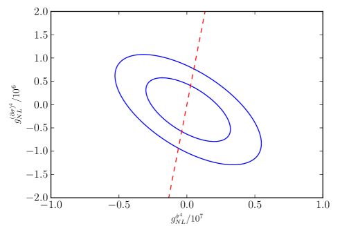
DBI Trispectrum: The trispectrum constraint on the shape in Eq. (82) can also be used to obtain a lower bound on the DBI model sound speed. This is because, in the small sound speed limit (Chen et al. 2009; Arroja et al. 2009), the dominant contribution to the contact interaction trispectrum (Huang & Shiu 2006) has this shape. The corresponding non-linearity parameter is . We follow the same procedure as described at the beginning of this section 11 and, assuming a uniform prior in the range , we can derive a constraint on as
| (121) |
This constraint is consistent with the ones derived from the bispectrum measurements (see Eqs. 96 and 97)) and it is only a factor of about three worse. Notice, however, that in this case we are ignoring the scalar exchange contribution, which is of the same order in .
Curvaton trispectrum: For the simplest curvaton scenario, the trispectrum non-linearity parameter prediction is (Sasaki et al. 2006)
| (122) |
Following the procedure described at the beginning of Sect. 11, we use the observational constraint obtained in Sect. 9 (Eq. 82), and the same prior () as in 11.2, to obtain a lower bound on the curvaton decay fraction as
| (123) |
This limit is consistent with the previous ones derived using the bispectrum measurements and it is a factor of about 3 to 4 worse.
12 Conclusions
In this paper we have presented the constraints on primordial NG using the full Planck mission data. The results have improved compared to the Planck 2013 release (Planck Collaboration XXIV 2014) as a consequence of including data from the full mission and taking advantage of Planck’s polarization capability — the first time that maps of the CMB polarization anisotropies have been used to constrain primordial NG.
Using temperature data alone, the constraints on the local, equilateral, and orthogonal bispectrum templates are , , and . Moving from the nominal Planck 2013 data to the full mission data yielded modest improvements of up to 15 % (for the orthogonal shape). After the inclusion of full mission polarization data, our final constraints become , , and , which represents a substantial step forward relative to Planck 2013, with error bars shrinking by 14 % (local), 43 % (equilateral), and 46 % (orthogonal). These improved limits on the standard shapes enhance our understanding of different inflationary models that can potentially lead to subtle effects beyond the simplest models of inflation.
The reason that the polarization data provide such complementary constraints on primordial curvature perturbations is due to the phase shift of the CMB polarization transfer functions compared to the temperature transfer functions. So, despite the relatively much lower signal-to-noise in the polarization maps, their inclusion leads to appreciable improvements on limits on NG parameters. Nevertheless, the full characterization of the noise properties in the polarized maps is still ongoing. In spite of the extensive testing and cross-checks validating the combined temperature and polarization results, we therefore conservatively recommend that all results that include polarization information, not just the polarization-only results, be taken as preliminary at this stage.
The complementary nature of the polarization information also represents an important cross-check on the analysis. The Planck results based on polarization alone are statistically consistent with the results based on temperature alone, with a precision comparable to that achievable in an optimal analysis of the WMAP 3-year temperature maps (Spergel et al. 2007; Creminelli et al. 2007; Yadav & Wandelt 2008).
Our analysis was subject to an extensive validation exercise. In addition to extensive simulation tests, including for the first time a detailed test of the impact of time-domain de-glitching, our results are supported by tests for robustness under change of estimator implementations (KSW, binned bispectrum, and two modal estimators), and variations in sky coverage as well as upper and lower multipole cutoffs. We also tested for possible directional dependence using a needlet estimator. These tests form the basis of our selection of SMICA as the main foreground cleaning method for our headline results.
The Planck 2015 analysis presented here provides constraints on a greatly extended range of template families. These extensions include a tenfold increase in the range of frequencies covered in feature models, giving rise to linearly oscillating bispectra, generalized shapes for oscillating models including for logarithmic oscillations, tests for deviations from the Bunch-Davies vacuum, models of equilateral type in the context of the effective field theory of inflation, and direction-dependent primordial NG. Beyond purely scalar mode templates we also tested for parity-violating tensor NG.
Using the full mission data with polarization, we have investigated the hints of NG reported in the Planck 2013 analysis of oscillatory features. While no individual feature or resonance model rises above our detection threshold of (after inclusion of the look-elsewhere effect), the results of integrated (multi-peak) statistical tests indicate that continued investigation of oscillatory and non-scaling models is warranted.
In addition to searches for specific NG templates, we present model-independent reconstructions of the temperature and polarization bispectra using the modal and binned bispectrum approaches. These full mission reconstructions can achieve twice the resolution of the Planck 2013 results, demonstrating excellent consistency in temperature, and good agreement with the WMAP9 reconstruction in regions where this earlier data set is signal-dominated.
The inclusion of polarization information leads to significantly improved constraints on NG in primordial isocurvature perturbations, providing complementary information to 2-point function results for models where the NG in isocurvature components is more easily detectable than its contribution to the power spectrum.
A significant addition to this year’s analysis is the inclusion of detailed trispectrum results due to cubic NG. The local trispectrum is constrained by Planck temperature data to be and the other two shapes were also found to be consistent with Gaussianity. Both 3-point and 4-point constraints are consistent with the improved (though still suboptimal) constraints from Minkowski functionals, a very different estimation framework. This concordance adds confidence in our results.
We have discussed the implications of our results on the physics of the early Universe, showing that the -point functions for provide a significant window onto the primordial Universe beyond the power spectrum, constraining general-single field, multifield, and non-standard inflation models, as well as alternatives to inflation. Using bispectrum and trispectrum limits we updated results on the parameter space of the inflationary models (and alternatives) already tested in 2013, and constrained the parameter space of other well-motivated inflationary models (e.g., Galileon-like models of inflation, and models where axion/pseudoscalar fields are present during inflation).
The global picture that emerges is one of consistency with the premises of the CDM cosmology, namely that the structure we observe today is the consequence of passive evolution of adiabatic, Gaussian, primordial seed perturbations. Nevertheless, NG at some level is expected in all inflationary models, and hence we should strive to find means to reduce errors on still further.
Acknowledgements.
The Planck Collaboration acknowledges the support of: ESA; CNES and CNRS/INSU-IN2P3-INP (France); ASI, CNR, and INAF (Italy); NASA and DoE (USA); STFC and UKSA (UK); CSIC, MINECO, JA, and RES (Spain); Tekes, AoF, and CSC (Finland); DLR and MPG (Germany); CSA (Canada); DTU Space (Denmark); SER/SSO (Switzerland); RCN (Norway); SFI (Ireland); FCT/MCTES (Portugal); ERC and PRACE (EU). A description of the Planck Collaboration and a list of its members, indicating which technical or scientific activities they have been involved in, can be found at http://www.cosmos.esa.int/web/planck/planck-collaboration. Some of the results in this paper have been derived using the HEALPix package. Part of this work was undertaken on the STFC COSMOS@DiRAC HPC Facility at the University of Cambridge, funded by UK BIS NEI grants. We gratefully acknowledge IN2P3 Computer Center (http://cc.in2p3.fr) for providing a significant amount of the computing resources and services needed for the analysis with the binned bispectrum estimator. This research used resources of the National Energy Research Scientific Computing Center, a DOE Office of Science User Facility supported by the Office of Science of the U.S. Department of Energy under Contract No. DE-AC02-05CH11231. We also acknowledge the IAP magique3 computer facilities. Some computations were performed on the GPC cluster at the SciNet HPC Consortium. SciNet is funded by the Canada Foundation for Innovation under the auspices of Compute Canada, the Government of Ontario, and the University of Toronto.References
- Achúcarro et al. (2011) Achúcarro, A., Gong, J.-O., Hardeman, S., Palma, G. A., & Patil, S. P., Features of heavy physics in the CMB power spectrum. 2011, J. Cosmology Astropart. Phys., 1, 30
- Achucarro et al. (2013) Achucarro, A., Gong, J.-O., Palma, G. A., & Patil, S. P., KachruCorrelating features in the primordial spectra. 2013, Phys.Rev., D87, 121301, 1211.5619
- Ackerman et al. (2007) Ackerman, L., Carroll, S. M., & Wise, M. B., Imprints of a primordial preferred direction on the microwave background. 2007, Phys. Rev. D, 75, 083502
- Acquaviva et al. (2003) Acquaviva, V., Bartolo, N., Matarrese, S., & Riotto, A., Gauge-invariant second-order perturbations and non-Gaussianity from inflation. 2003, Nuclear Physics B, 667, 119
- Adshead et al. (2012) Adshead, P., Dvorkin, C., Hu, W., & Lim, E. A., Non-Gaussianity from step features in the inflationary potential. 2012, Phys. Rev. D, 85, 023531
- Adshead et al. (2011) Adshead, P., Hu, W., Dvorkin, C., & Peiris, H. V., Fast Computation of Bispectrum Features with Generalized Slow Roll. 2011, Phys. Rev. D, 84, 043519
- Agullo & Parker (2011) Agullo, I. & Parker, L., Stimulated creation of quanta during inflation and the observable universe. 2011, General Relativity and Gravitation, 43, 2541
- Alishahiha et al. (2004) Alishahiha, M., Silverstein, E., & Tong, D., DBI in the sky: Non-Gaussianity from inflation with a speed limit. 2004, Phys. Rev. D, 70, 123505
- Argüeso et al. (2003) Argüeso, F., González-Nuevo, J., & Toffolatti, L., Contributions of Point Extragalactic Sources to the Cosmic Microwave Background Bispectrum. 2003, ApJ, 598, 86, arXiv:astro-ph/0307148
- Arkani-Hamed et al. (2004) Arkani-Hamed, N., Creminelli, P., Mukohyama, S., & Zaldarriaga, M., Ghost inflation. 2004, J. Cosmology Astropart. Phys., 4, 1
- Arroja et al. (2013) Arroja, F., Bartolo, N., Dimastrogiovanni, E., & Fasiello, M., On the Trispectrum of Galileon Inflation. 2013, JCAP, 1311, 005, 1307.5371
- Arroja et al. (2009) Arroja, F., Mizuno, S., Koyama, K., & Tanaka, T., Full trispectrum in single field DBI inflation. 2009, Phys. Rev. D, 80, 043527
- Ashoorioon & Shiu (2011) Ashoorioon, A. & Shiu, G., A Note on Calm Excited States of Inflation. 2011, JCAP, 1103, 025, 1012.3392
- Babich et al. (2004) Babich, D., Creminelli, P., & Zaldarriaga, M., The shape of non-Gaussianities. 2004, J. Cosmology Astropart. Phys., 8, 9
- Bardeen (1980) Bardeen, J. M., Gauge-invariant cosmological perturbations. 1980, Phys. Rev. D, 22, 1882
- Barnaby & Cline (2006) Barnaby, N. & Cline, J. M., Non-Gaussian and nonscale-invariant perturbations from tachyonic preheating in hybrid inflation. 2006, Phys. Rev. D, 73, 106012
- Barnaby et al. (2012a) Barnaby, N., Moxon, J., Namba, R., et al., Gravity waves and non-Gaussian features from particle production in a sector gravitationally coupled to the inflaton. 2012a, Phys. Rev. D, 86, 103508, 1206.6117
- Barnaby et al. (2011) Barnaby, N., Namba, R., & Peloso, M., Phenomenology of a pseudo-scalar inflaton: naturally large nongaussianity. 2011, J. Cosmology Astropart. Phys., 4, 9
- Barnaby et al. (2012b) Barnaby, N., Namba, R., & Peloso, M., Observable non-Gaussianity from gauge field production in slow roll inflation, and a challenging connection with magnetogenesis. 2012b, Phys. Rev. D, 85, 123523
- Barnaby et al. (2012c) Barnaby, N., Pajer, E., & Peloso, M., Gauge field production in axion inflation: Consequences for monodromy, non-Gaussianity in the CMB, and gravitational waves at interferometers. 2012c, Phys. Rev. D, 85, 023525
- Barnaby & Peloso (2011) Barnaby, N. & Peloso, M., Large Non-Gaussianity in Axion Inflation. 2011, Physical Review Letters, 106, 181301
- Bartolo et al. (2013) Bartolo, N., Dimastrogiovanni, E., & Fasiello, M., The Trispectrum in the Effective Theory of Inflation with Galilean symmetry. 2013, JCAP, 1309, 037, 1305.0812
- Bartolo et al. (2010a) Bartolo, N., Fasiello, M., Matarrese, S., & Riotto, A., Large non-Gaussianities in the effective field theory approach to single-field inflation: the bispectrum. 2010a, J. Cosmology Astropart. Phys., 8, 8
- Bartolo et al. (2010b) Bartolo, N., Fasiello, M., Matarrese, S., & Riotto, A., Large non-Gaussianities in the effective field theory approach to single-field inflation: the trispectrum. 2010b, J. Cosmology Astropart. Phys., 9, 35
- Bartolo et al. (2004a) Bartolo, N., Komatsu, E., Matarrese, S., & Riotto, A., Non-Gaussianity from inflation: theory and observations. 2004a, Phys. Rep, 402, 103
- Bartolo et al. (2013a) Bartolo, N., Matarrese, S., Peloso, M., & Ricciardone, A., Anisotropic power spectrum and bispectrum in the f()F2 mechanism. 2013a, Phys. Rev. D, 87, 023504
- Bartolo et al. (2013b) Bartolo, N., Matarrese, S., Peloso, M., & Ricciardone, A., Anisotropy in solid inflation. 2013b, J. Cosmology Astropart. Phys., 8, 22, 1306.4160
- Bartolo et al. (2002) Bartolo, N., Matarrese, S., & Riotto, A., Non-Gaussianity from inflation. 2002, Phys. Rev. D, 65, 103505
- Bartolo et al. (2004b) Bartolo, N., Matarrese, S., & Riotto, A., Gauge-Invariant Temperature Anisotropies and Primordial Non-Gaussianity. 2004b, Physical Review Letters, 93, 231301
- Bartolo et al. (2004c) Bartolo, N., Matarrese, S., & Riotto, A., Non-Gaussianity in the curvaton scenario. 2004c, Phys. Rev. D, 69, 043503
- Bartolo et al. (2014) Bartolo, N., Peloso, M., Ricciardone, A., & Unal, C., The expected anisotropy in solid inflation. 2014, J. Cosmology Astropart. Phys., 11, 9, 1407.8053
- Bastero-Gil et al. (2014) Bastero-Gil, M., Berera, A., Moss, I. G., & Ramos, R. O., Theory of non-Gaussianity in warm inflation. 2014, J. Cosmology Astropart. Phys., 12, 8, 1408.4391
- Battefeld et al. (2013) Battefeld, T., Niemeyer, J. C., & Vlaykov, D., Probing two-field open inflation by resonant signals in correlation functions. 2013, J. Cosmology Astropart. Phys., 5, 6, 1302.3877
- Baumann & Green (2012) Baumann, D. & Green, D., Signature of supersymmetry from the early universe. 2012, Phys. Rev. D, 85, 103520
- Bean et al. (2008) Bean, R., Chen, X., Peiris, H., & Xu, J., Comparing infrared Dirac-Born-Infeld brane inflation to observations. 2008, Phys. Rev. D, 77, 023527
- Behbahani et al. (2012) Behbahani, S. R., Dymarsky, A., Mirbabayi, M., & Senatore, L., (Small) Resonant non-Gaussianities: Signatures of a Discrete Shift Symmetry in the Effective Field Theory of Inflation. 2012, JCAP, 1212, 036, 1111.3373
- Bennett et al. (2013) Bennett, C. L., Larson, D., Weiland, J. L., et al., Nine-year Wilkinson Microwave Anisotropy Probe (WMAP) Observations: Final Maps and Results. 2013, ApJS, 208, 20
- Bernardeau et al. (2004) Bernardeau, F., Kofman, L., & Uzan, J.-P., Modulated fluctuations from hybrid inflation. 2004, Phys. Rev. D, 70, 083004
- Bernardeau & Uzan (2002) Bernardeau, F. & Uzan, J.-P., Non-Gaussianity in multifield inflation. 2002, Phys. Rev. D, 66, 103506
- Bond et al. (2009) Bond, J. R., Frolov, A. V., Huang, Z., & Kofman, L., Non-Gaussian Curvature Spikes from Chaotic Billiards in Inflation Preheating. 2009, Physical Review Letters, 103, 071301
- Brown & Crittenden (2005) Brown, I. & Crittenden, R., Non-Gaussianity from cosmic magnetic fields. 2005, Phys. Rev. D, 72, 063002, astro-ph/0506570
- Bucher et al. (2000) Bucher, M., Moodley, K., & Turok, N., General primordial cosmic perturbation. 2000, Phys. Rev. D, 62, 083508, astro-ph/9904231
- Bucher et al. (2016) Bucher, M., Racine, B., & van Tent, B., The binned bispectrum estimator: template-based and non-parametric CMB non-Gaussianity searches. 2016, J. Cosmology Astropart. Phys., 5, 055, 1509.08107
- Bucher et al. (2010) Bucher, M., van Tent, B., & Carvalho, C. S., Detecting bispectral acoustic oscillations from inflation using a new flexible estimator. 2010, MNRAS, 407, 2193
- Burrage et al. (2011) Burrage, C., de Rham, C., Seery, D., & Tolley, A. J., Galileon inflation. 2011, J. Cosmology Astropart. Phys., 1, 14, 1009.2497
- Byrnes & Choi (2010) Byrnes, C. T. & Choi, K.-Y., Review of Local Non-Gaussianity from Multifield Inflation. 2010, Advances in Astronomy, 2010
- Catalano et al. (2014) Catalano, A., Ade, P., Atik, Y., et al., Impact of particles on the Planck HFI detectors: Ground-based measurements and physical interpretation. 2014, ArXiv e-prints, 1403.6592
- Chambers & Rajantie (2008) Chambers, A. & Rajantie, A., Lattice Calculation of Non-Gaussian Density Perturbations from the Massless Preheating Inflationary Model. 2008, Physical Review Letters, 100, 041302
- Chen (2005a) Chen, X., Inflation from warped space. 2005a, Journal of High Energy Physics, 8, 45
- Chen (2005b) Chen, X., Multithroat brane inflation. 2005b, Phys. Rev. D, 71, 063506
- Chen (2010a) Chen, X., Folded resonant non-Gaussianity in general single field inflation. 2010a, J. Cosmology Astropart. Phys., 12, 3
- Chen (2010b) Chen, X., Primordial Non-Gaussianities from Inflation Models. 2010b, Advances in Astronomy, 2010
- Chen (2011) Chen, X., Primordial Features as Evidence for Inflation. 2011, ArXiv e-prints, 1104.1323
- Chen et al. (2007a) Chen, X., Easther, R., & Lim, E. A., Large non-Gaussianities in single-field inflation. 2007a, J. Cosmology Astropart. Phys., 6, 23
- Chen et al. (2008) Chen, X., Easther, R., & Lim, E. A., Generation and characterization of large non-Gaussianities in single field inflation. 2008, J. Cosmology Astropart. Phys., 4, 10
- Chen et al. (2009) Chen, X., Hu, B., Huang, M.-x., Shiu, G., & Wang, Y., Large primordial trispectra in general single field inflation. 2009, J. Cosmology Astropart. Phys., 8, 8
- Chen et al. (2007b) Chen, X., Huang, M.-x., Kachru, S., & Shiu, G., Observational signatures and non-Gaussianities of general single-field inflation. 2007b, J. Cosmology Astropart. Phys., 1, 2
- Chen et al. (2015) Chen, X., Namjoo, M. H., & Wang, Y., Models of the Primordial Standard Clock. 2015, J. Cosmology Astropart. Phys., 2, 27, 1411.2349
- Chen & Wang (2010) Chen, X. & Wang, Y., Quasi-single field inflation and non-Gaussianities. 2010, J. Cosmology Astropart. Phys., 4, 27
- Cheung et al. (2008) Cheung, C., Fitzpatrick, A. L., Kaplan, J., Senatore, L., & Creminelli, P., The effective field theory of inflation. 2008, Journal of High Energy Physics, 3, 14
- Cicoli et al. (2012) Cicoli, M., Tasinato, G., Zavala, I., Burgess, C. P., & Quevedo, F., Modulated reheating and large non-gaussianity in string cosmology. 2012, J. Cosmology Astropart. Phys., 5, 39
- Cook & Sorbo (2013) Cook, J. L. & Sorbo, L., An inflationary model with small scalar and large tensor nongaussianities. 2013, J. Cosmology Astropart. Phys., 11, 47, 1307.7077
- Cooray & Melchiorri (2006) Cooray, A. & Melchiorri, A., Searching for integrated Sachs Wolfe effect beyond temperature anisotropies: CMB E-mode polarization galaxy cross-correlation. 2006, Journal of Cosmology and Astro-Particle Physics, 1, 18, arXiv:astro-ph/0511054
- Crawford et al. (2014) Crawford, T. M., Schaffer, K. K., Bhattacharya, S., et al., A Measurement of the Secondary-CMB and Millimeter-wave-foreground Bispectrum using 800 deg2 of South Pole Telescope Data. 2014, ApJ, 784, 143, 1303.3535
- Creminelli et al. (2011) Creminelli, P., D’Amico, G., Musso, M., Noreña, J., & Trincherini, E., Galilean symmetry in the effective theory of inflation: new shapes of non-Gaussianity. 2011, J. Cosmology Astropart. Phys., 2, 6, 1011.3004
- Creminelli et al. (2006) Creminelli, P., Nicolis, A., Senatore, L., Tegmark, M., & Zaldarriaga, M., Limits on non-Gaussianities from WMAP data. 2006, J. Cosmology Astropart. Phys., 5, 4
- Creminelli et al. (2007) Creminelli, P., Senatore, L., Zaldarriaga, M., & Tegmark, M., Limits on fNL parameters from Wilkinson Microwave Anisotropy Probe three-year data. 2007, J. Cosmology Astropart. Phys., 3, 5, astro-ph/0610600
- Curto et al. (2008) Curto, A., Macias-Perez, J. F., Martínez-González, E., et al., Constraints on the non-linear coupling parameter f_nl with Archeops data. 2008, A&A, 486, 383
- Curto et al. (2014) Curto, A., Tucci, M., Kunz, M., & Martinez-Gonzalez, E., The CIB-lensing bispectrum: impact on primordial non-Gaussianity and detectability for the Planck mission. 2014, ArXiv e-prints, 1405.7029
- de Rham & Gabadadze (2010a) de Rham, C. & Gabadadze, G., Generalization of the Fierz-Pauli action. 2010a, Phys. Rev. D, 82, 044020, 1007.0443
- de Rham & Gabadadze (2010b) de Rham, C. & Gabadadze, G., Selftuned massive spin-2. 2010b, Physics Letters B, 693, 334, 1006.4367
- Delabrouille et al. (2013) Delabrouille, J., Betoule, M., Melin, J.-B., et al., The pre-launch Planck Sky Model: a model of sky emission at submillimetre to centimetre wavelengths. 2013, A&A, 553, A96, 1207.3675
- Desjacques & Seljak (2010) Desjacques, V. & Seljak, U., Signature of primordial non-Gaussianity of phi3-type in the mass function and bias of dark matter haloes. 2010, Phys.Rev., D81, 023006, 0907.2257
- Donzelli et al. (2012) Donzelli, S., Hansen, F. K., Liguori, M., Marinucci, D., & Matarrese, S., On the Linear Term Correction for Needlet/Wavelet Non-Gaussianity Estimators. 2012, ApJ, 755, 19, 1202.1478
- Ducout et al. (2013) Ducout, A., Bouchet, F. R., Colombi, S., Pogosyan, D., & Prunet, S., Non-Gaussianity and Minkowski functionals: forecasts for Planck. 2013, MNRAS, 429, 2104
- Dvali et al. (2004a) Dvali, G., Gruzinov, A., & Zaldarriaga, M., Cosmological perturbations from inhomogeneous reheating, freeze-out, and mass domination. 2004a, Phys. Rev. D, 69, 083505
- Dvali et al. (2004b) Dvali, G., Gruzinov, A., & Zaldarriaga, M., New mechanism for generating density perturbations from inflation. 2004b, Phys. Rev. D, 69, 023505
- Elsner & Wandelt (2009) Elsner, F. & Wandelt, B. D., Improved Simulation of Non-Gaussian Temperature and Polarization Cosmic Microwave Background Maps. 2009, ApJS, 184, 264
- Elsner & Wandelt (2012) Elsner, F. & Wandelt, B. D., Fast Wiener filtering of CMB maps. 2012, ArXiv e-prints, 1211.0585
- Endlich et al. (2014) Endlich, S., Horn, B., Nicolis, A., & Wang, J., Squeezed limit of the solid inflation three-point function. 2014, Phys. Rev. D, 90, 063506, 1307.8114
- Endlich et al. (2013) Endlich, S., Nicolis, A., & Wang, J., Solid inflation. 2013, J. Cosmology Astropart. Phys., 10, 11
- Enqvist et al. (2005) Enqvist, K., Jokinen, A., Mazumdar, A., Multamäki, T., & Väihkönen, A., Non-Gaussianity from preheating. 2005, Physical Review Letters, 94, 161301
- Enqvist & Sloth (2002) Enqvist, K. & Sloth, M. S., Adiabatic CMB perturbations in pre-Big-Bang string cosmology. 2002, Nuclear Physics B, 626, 395
- Eriksen et al. (2004) Eriksen, H. K., Novikov, D. I., Lilje, P. B., Banday, A. J., & Górski, K. M., Testing for Non-Gaussianity in the Wilkinson Microwave Anisotropy Probe Data: Minkowski Functionals and the Length of the Skeleton. 2004, ApJ, 612, 64
- Falk et al. (1993) Falk, T., Rangarajan, R., & Srednicki, M., The angular dependence of the three-point correlation function of the cosmic microwave background radiation as predicted by inflationary cosmologies. 1993, ApJ, 403, L1
- Fantaye et al. (2015) Fantaye, Y., Marinucci, D., Hansen, F., & Maino, D., Applications of the Gaussian kinematic formula to CMB data analysis. 2015, Phys. Rev. D, 91, 063501
- Feng et al. (2015) Feng, C., Cooray, A., Smidt, J., et al., Planck Trispectrum Constraints on Primordial Non-Gaussianity at Cubic Order. 2015, 1502.00585
- Fergusson (2014) Fergusson, J., Efficient optimal non-Gaussian CMB estimators with polarisation. 2014, Phys.Rev., D90, 043533, 1403.7949
- Fergusson et al. (2015) Fergusson, J., Gruetjen, H., Shellard, E., & Liguori, M., Combining power spectrum and bispectrum measurements to detect oscillatory features. 2015, Phys.Rev., D91, 023502, 1410.5114
- Fergusson et al. (2014) Fergusson, J., Gruetjen, H., Shellard, E., & Wallisch, B., Polyspectra searches for sharp oscillatory features in cosmic microwave sky data. 2014, 1412.6152
- Fergusson et al. (2010a) Fergusson, J. R., Liguori, M., & Shellard, E. P. S., General CMB and primordial bispectrum estimation: Mode expansion, map making, and measures of FNL. 2010a, Phys. Rev. D, 82, 023502
- Fergusson et al. (2012) Fergusson, J. R., Liguori, M., & Shellard, E. P. S., The CMB bispectrum. 2012, J. Cosmology Astropart. Phys., 12, 32, 1006.1642
- Fergusson et al. (2010b) Fergusson, J. R., Regan, D. M., & Shellard, E. P. S., Optimal Trispectrum Estimators and WMAP Constraints. 2010b, ArXiv e-prints, 1012.6039
- Ferreira & Sloth (2014) Ferreira, R. Z. & Sloth, M. S., Universal Constraints on Axions from Inflation. 2014, ArXiv e-prints, 1409.5799
- Fertig et al. (2014) Fertig, A., Lehners, J.-L., & Mallwitz, E., Ekpyrotic Perturbations With Small Non-Gaussian Corrections. 2014, Phys.Rev., D89, 103537, 1310.8133
- Flauger et al. (2010) Flauger, R., McAllister, L., Pajer, E., Westphal, A., & Xu, G., Oscillations in the CMB from axion monodromy inflation. 2010, J. Cosmology Astropart. Phys., 6, 9
- Flauger & Pajer (2011) Flauger, R. & Pajer, E., Resonant non-gaussianity. 2011, J. Cosmology Astropart. Phys., 1, 17
- Gangui et al. (1994) Gangui, A., Lucchin, F., Matarrese, S., & Mollerach, S., The three-point correlation function of the cosmic microwave background in inflationary models. 1994, ApJ, 430, 447
- Gangui & Martin (2000) Gangui, A. & Martin, J., Cosmic microwave background bispectrum and slow-roll inflation. 2000, MNRAS, 313, 323
- Gao et al. (2011) Gao, X., Kobayashi, T., Yamaguchi, M., & Yokoyama, J., Primordial Non-Gaussianities of Gravitational Waves in the Most General Single-Field Inflation Model with Second-Order Field Equations. 2011, Physical Review Letters, 107, 211301, 1108.3513
- Giannantonio et al. (2014) Giannantonio, T., Ross, A. J., Percival, W. J., et al., Improved Primordial Non-Gaussianity Constraints from Measurements of Galaxy Clustering and the Integrated Sachs-Wolfe Effect. 2014, Phys.Rev., D89, 023511, 1303.1349
- González-Nuevo et al. (2005) González-Nuevo, J., Toffolatti, L., & Argüeso, F., Predictions of the Angular Power Spectrum of Clustered Extragalactic Point Sources at Cosmic Microwave Background Frequencies from Flat and All-Sky Two-dimensional Simulations. 2005, ApJ, 621, 1
- Górski et al. (2005) Górski, K. M., Hivon, E., Banday, A. J., et al., HEALPix: A Framework for High-Resolution Discretization and Fast Analysis of Data Distributed on the Sphere. 2005, ApJ, 622, 759, astro-ph/0409513
- Hall & Peiris (2008) Hall, L. M. H. & Peiris, H. V., Cosmological constraints on dissipative models of inflation. 2008, J. Cosmology Astropart. Phys., 1, 27
- Hannestad et al. (2010) Hannestad, S., Haugbolle, T., Jarnhus, P. R., & Sloth, M. S., Non-Gaussianity from Axion Monodromy Inflation. 2010, JCAP, 1006, 001, 0912.3527
- Hanson & Lewis (2009) Hanson, D. & Lewis, A., Estimators for CMB statistical anisotropy. 2009, Phys. Rev. D, 80, 063004
- Heavens (1998) Heavens, A. F., Estimating non-Gaussianity in the microwave background. 1998, MNRAS, 299, 805
- Hikage et al. (2013a) Hikage, C., Kawasaki, M., Sekiguchi, T., & Takahashi, T., CMB constraint on non-Gaussianity in isocurvature perturbations. 2013a, J. Cosmology Astropart. Phys., 7, 7, 1211.1095
- Hikage et al. (2013b) Hikage, C., Kawasaki, M., Sekiguchi, T., & Takahashi, T., Extended analysis of CMB constraints on non-gaussianity in isocurvature perturbations. 2013b, J. Cosmology Astropart. Phys., 3, 20, 1212.6001
- Hikage et al. (2006) Hikage, C., Komatsu, E., & Matsubara, T., Primordial Non-Gaussianity and Analytical Formula for Minkowski Functionals of the Cosmic Microwave Background and Large-Scale Structure. 2006, ApJ, 653, 11
- Hikage et al. (2009) Hikage, C., Koyama, K., Matsubara, T., Takahashi, T., & Yamaguchi, M., Limits on isocurvature perturbations from non-Gaussianity in WMAP temperature anisotropy. 2009, MNRAS, 398, 2188, 0812.3500
- Hikage & Matsubara (2012) Hikage, C. & Matsubara, T., Limits on second-order non-Gaussianity from Minkowski functionals of WMAP 7-year data. 2012, MNRAS, 425, 2187
- Hikage et al. (2008) Hikage, C., Matsubara, T., Coles, P., et al., Limits on primordial non-Gaussianity from Minkowski Functionals of the WMAP temperature anisotropies. 2008, MNRAS, 389, 1439
- Holman & Tolley (2008) Holman, R. & Tolley, A. J., Enhanced Non-Gaussianity from Excited Initial States. 2008, JCAP, 0805, 001, 0710.1302
- Horndeski (1974) Horndeski, G. W., Second-Order Scalar-Tensor Field Equations in a Four-Dimensional Space. 1974, International Journal of Theoretical Physics, 10, 363
- Hu (2000) Hu, W., Weak lensing of the CMB: A harmonic approach. 2000, Phys. Rev. D, 62, 043007, astro-ph/0001303
- Huang & Shiu (2006) Huang, M.-X. & Shiu, G., Inflationary trispectrum for models with large non-Gaussianities. 2006, Phys. Rev. D, 74, 121301, hep-th/0610235
- Kamionkowski & Souradeep (2011) Kamionkowski, M. & Souradeep, T., Odd-parity cosmic microwave background bispectrum. 2011, Phys. Rev. D, 83, 027301, 1010.4304
- Kawakami et al. (2012) Kawakami, E., Kawasaki, M., Miyamoto, K., Nakayama, K., & Sekiguchi, T., Non-Gaussian isocurvature perturbations in dark radiation. 2012, J. Cosmology Astropart. Phys., 7, 37, 1202.4890
- Kawasaki et al. (2008) Kawasaki, M., Nakayama, K., Sekiguchi, T., Suyama, T., & Takahashi, F., Non-Gaussianity from isocurvature perturbations. 2008, J. Cosmology Astropart. Phys., 11, 19, 0808.0009
- Kawasaki et al. (2009) Kawasaki, M., Nakayama, K., Sekiguchi, T., Suyama, T., & Takahashi, F., A general analysis of non-gaussianity from isocurvature perturbations. 2009, J. Cosmology Astropart. Phys., 1, 42, 0810.0208
- Kobayashi et al. (2010) Kobayashi, T., Yamaguchi, M., & Yokoyama, J., Inflation Driven by the Galileon Field. 2010, Physical Review Letters, 105, 231302, 1008.0603
- Kofman (2003) Kofman, L., Probing String Theory with Modulated Cosmological Fluctuations. 2003, ArXiv Astrophysics e-prints, arXiv:astro-ph/0303614
- Kolb et al. (2006) Kolb, E. W., Riotto, A., & Vallinotto, A., Non-Gaussianity from broken symmetries. 2006, Phys. Rev. D, 73, 023522
- Komatsu (2002) Komatsu, E., The Pursuit of Non-Gaussian Fluctuations in the Cosmic Microwave Background. 2002, ArXiv Astrophysics e-prints, astro-ph/0206039
- Komatsu (2010) Komatsu, E., Hunting for primordial non-Gaussianity in the cosmic microwave background. 2010, Classical and Quantum Gravity, 27, 124010
- Komatsu & Spergel (2001) Komatsu, E. & Spergel, D. N., Acoustic signatures in the primary microwave background bispectrum. 2001, Phys. Rev. D, 63, 063002
- Komatsu et al. (2005) Komatsu, E., Spergel, D. N., & Wandelt, B. D., Measuring Primordial Non-Gaussianity in the Cosmic Microwave Background. 2005, ApJ, 634, 14
- Koyama et al. (2007) Koyama, K., Mizuno, S., Vernizzi, F., & Wands, D., Non-Gaussianities from ekpyrotic collapse with multiple fields. 2007, JCAP, 0711, 024, 0708.4321
- Lacasa & Aghanim (2014) Lacasa, F. & Aghanim, N., Optimal estimator for the amplitude of the bispectrum from infrared clustered sources. 2014, A&A, 569, A51
- Lacasa et al. (2012) Lacasa, F., Aghanim, N., Kunz, M., & Frommert, M., Characterization of the non-Gaussianity of radio and IR point sources at CMB frequencies. 2012, MNRAS, 421, 1982
- Lacasa et al. (2014) Lacasa, F., Pénin, A., & Aghanim, N., Non-Gaussianity of the cosmic infrared background anisotropies - I. Diagrammatic formalism and application to the angular bispectrum. 2014, MNRAS, 439, 123, 1312.1251
- Lagache et al. (2005) Lagache, G., Puget, J.-L., & Dole, H., Dusty Infrared Galaxies: Sources of the Cosmic Infrared Background. 2005, ARA&A, 43, 727, arXiv:astro-ph/0507298
- Lan & Marinucci (2008) Lan, X. & Marinucci, D., The needlets bispectrum. 2008, Electronic Journal of Statistics, 2, 332, 0802.4020
- Langlois & Lepidi (2011) Langlois, D. & Lepidi, A., General treatment of isocurvature perturbations and non-Gaussianities. 2011, J. Cosmology Astropart. Phys., 1, 8, 1007.5498
- Langlois & van Tent (2011) Langlois, D. & van Tent, B., Hunting for isocurvature modes in the cosmic microwave background non-Gaussianities. 2011, Classical and Quantum Gravity, 28, 222001, 1104.2567
- Langlois & van Tent (2012) Langlois, D. & van Tent, B., Isocurvature modes in the CMB bispectrum. 2012, J. Cosmology Astropart. Phys., 7, 40, 1204.5042
- Langlois et al. (2008) Langlois, D., Vernizzi, F., & Wands, D., Non-linear isocurvature perturbations and non-Gaussianities. 2008, J. Cosmology Astropart. Phys., 12, 4, 0809.4646
- Lehners (2010) Lehners, J.-L., Ekpyrotic Nongaussianity: A Review. 2010, Advances in Astronomy, 2010
- Lehners & Steinhardt (2008) Lehners, J.-L. & Steinhardt, P. J., Non-Gaussian density fluctuations from entropically generated curvature perturbations in Ekpyrotic models. 2008, Phys.Rev., D77, 063533, 0712.3779
- Lehners & Steinhardt (2013) Lehners, J.-L. & Steinhardt, P. J., Planck 2013 results support the cyclic universe. 2013, Phys.Rev., D87, 123533, 1304.3122
- Leistedt et al. (2014) Leistedt, B., Peiris, H. V., & Roth, N., Constraints on Primordial Non-Gaussianity from 800 000 Photometric Quasars. 2014, Phys.Rev.Lett., 113, 221301, 1405.4315
- Lewis et al. (2011) Lewis, A., Challinor, A., & Hanson, D., The shape of the CMB lensing bispectrum. 2011, J. Cosmology Astropart. Phys., 3, 18
- Li (2013) Li, M., Note on the production of scale-invariant entropy perturbation in the Ekpyrotic universe. 2013, Phys.Lett., B724, 192, 1306.0191
- Liguori et al. (2010) Liguori, M., Sefusatti, E., Fergusson, J. R., & Shellard, E. P. S., Primordial Non-Gaussianity and Bispectrum Measurements in the Cosmic Microwave Background and Large-Scale Structure. 2010, Advances in Astronomy, 2010
- Liguori et al. (2015) Liguori, M., Shiraishi, M., Fergusson, J., & Shellard, E., . 2015, In prep.
- Linde et al. (2013) Linde, A., Mooij, S., & Pajer, E., Gauge field production in supergravity inflation: Local non-Gaussianity and primordial black holes. 2013, Phys. Rev. D, 87, 103506, 1212.1693
- Linde & Mukhanov (1997) Linde, A. & Mukhanov, V., Non-Gaussian isocurvature perturbations from inflation. 1997, Phys. Rev. D, 56, 535
- Linde & Mukhanov (2006) Linde, A. & Mukhanov, V., The curvaton web. 2006, J. Cosmology Astropart. Phys., 4, 9, astro-ph/0511736
- Lyth (2005) Lyth, D. H., Generating the curvature perturbation at the end of inflation. 2005, J. Cosmology Astropart. Phys., 11, 6
- Lyth & Riotto (2006) Lyth, D. H. & Riotto, A., Generating the Curvature Perturbation at the End of Inflation in String Theory. 2006, Physical Review Letters, 97, 121301
- Lyth & Rodriguez (2005) Lyth, D. H. & Rodriguez, Y., Inflationary Prediction for Primordial Non-Gaussianity. 2005, Physical Review Letters, 95, 121302
- Lyth et al. (2003) Lyth, D. H., Ungarelli, C., & Wands, D., Primordial density perturbation in the curvaton scenario. 2003, Phys. Rev. D, 67, 023503
- Lyth & Wands (2002) Lyth, D. H. & Wands, D., Generating the curvature perturbation without an inflaton. 2002, Physics Letters B, 524, 5
- Maldacena (2003) Maldacena, J., Non-gaussian features of primordial fluctuations in single field inflationary models. 2003, Journal of High Energy Physics, 5, 13
- Maldacena & Pimentel (2011) Maldacena, J. M. & Pimentel, G. L., On graviton non-gaussianities during inflation. 2011, Journal of High Energy Physics, 9, 45, 1104.2846
- Malik & Lyth (2006) Malik, K. A. & Lyth, D. H., A numerical study of non-Gaussianity in the curvaton scenario. 2006, J. Cosmology Astropart. Phys., 9, 8
- Mangilli & Verde (2009) Mangilli, A. & Verde, L., Non-Gaussianity and the CMB bispectrum: Confusion between primordial and lensing-Rees-Sciama contribution? 2009, Phys. Rev. D, 80, 123007, 0906.2317
- Mangilli et al. (2013) Mangilli, A., Wandelt, B., Elsner, F., & Liguori, M., Optimal bispectrum estimator and simulations of the CMB lensing-integrated Sachs Wolfe non-Gaussian signal. 2013, A&A, 555, A82
- Matsubara (2010) Matsubara, T., Analytic Minkowski functionals of the cosmic microwave background: Second-order non-Gaussianity with bispectrum and trispectrum. 2010, Phys. Rev. D, 81, 083505
- McFadden & Skenderis (2011) McFadden, P. & Skenderis, K., Cosmological 3-point correlators from holography. 2011, J. Cosmology Astropart. Phys., 6, 30, 1104.3894
- Mecke et al. (1994) Mecke, K. R., Buchert, T., & Wagner, H., Robust morphological measures for large-scale structure in the Universe. 1994, A&A, 288, 697, arXiv:astro-ph/9312028
- Meerburg et al. (2015) Meerburg, P. D., Münchmeyer, M., & Wandelt, B., Joint resonant CMB power spectrum and bispectrum estimation. 2015, 1510.01756
- Meerburg & Pajer (2013) Meerburg, P. D. & Pajer, E., Observational constraints on gauge field production in axion inflation. 2013, J. Cosmology Astropart. Phys., 2, 17, 1203.6076
- Meerburg et al. (2009) Meerburg, P. D., van der Schaar, J. P., & Stefano Corasaniti, P., Signatures of initial state modifications on bispectrum statistics. 2009, J. Cosmology Astropart. Phys., 5, 18
- Mizuno & Koyama (2010) Mizuno, S. & Koyama, K., Primordial non-Gaussianity from the DBI Galileons. 2010, Phys. Rev. D, 82, 103518, 1009.0677
- Modest et al. (2013) Modest, H. I., Räth, C., Banday, A. J., et al., Scale-dependent non-Gaussianities in the CMB data identified with Minkowski functionals and scaling indices. 2013, MNRAS, 428, 551
- Mollerach (1990) Mollerach, S., Isocurvature baryon perturbations and inflation. 1990, Phys. Rev. D, 42, 313
- Moroi & Takahashi (2001) Moroi, T. & Takahashi, T., Effects of cosmological moduli fields on cosmic microwave background. 2001, Physics Letters B, 522, 215
- Moss & Xiong (2007) Moss, I. G. & Xiong, C., Non-Gaussianity in fluctuations from warm inflation. 2007, J. Cosmology Astropart. Phys., 4, 7
- Münchmeyer et al. (2014) Münchmeyer, M., Bouchet, F., Jackson, M., & Wandelt, B., The Komatsu Spergel Wandelt estimator for oscillations in the cosmic microwave background bispectrum. 2014, Astron.Astrophys., 570, A94, 1405.2550
- Münchmeyer et al. (2015) Münchmeyer, M., Meerburg, P. D., & Wandelt, B. D., Optimal estimator for resonance bispectra in the CMB. 2015, Phys.Rev., D91, 043534, 1412.3461
- Munshi & Heavens (2010) Munshi, D. & Heavens, A., A new approach to probing primordial non-Gaussianity. 2010, MNRAS, 401, 2406
- Munshi et al. (2013) Munshi, D., Smidt, J., Cooray, A., et al., New approaches to probing Minkowski functionals. 2013, MNRAS, 434, 2830, 1011.5224
- Natoli et al. (2010) Natoli, P., de Troia, G., Hikage, C., et al., BOOMERanG constraints on primordial non-Gaussianity from analytical Minkowski functionals. 2010, MNRAS, 408, 1658
- Nicolis et al. (2009) Nicolis, A., Rattazzi, R., & Trincherini, E., Galileon as a local modification of gravity. 2009, Phys. Rev. D, 79, 064036, 0811.2197
- Novaes et al. (2014) Novaes, C. P., Bernui, A., Ferreira, I. S., & Wuensche, C. A., A Neural-Network based estimator to search for primordial non-Gaussianity in Planck CMB maps. 2014, ArXiv e-prints, 1409.3876
- Ohashi & Tsujikawa (2012) Ohashi, J. & Tsujikawa, S., Potential-driven Galileon inflation. 2012, J. Cosmology Astropart. Phys., 10, 35, 1207.4879
- Okamoto & Hu (2002) Okamoto, T. & Hu, W., Angular trispectra of CMB temperature and polarization. 2002, Phys. Rev. D, 66, 063008
- Park et al. (2005) Park, C., Choi, Y.-Y., Vogeley, M. S., et al., Topology Analysis of the Sloan Digital Sky Survey. I. Scale and Luminosity Dependence. 2005, ApJ, 633, 11, arXiv:astro-ph/0507059
- Pénin et al. (2014) Pénin, A., Lacasa, F., & Aghanim, N., Non-Gaussianity of the cosmic infrared background anisotropies - II. Predictions of the bispectrum and constraints forecast. 2014, MNRAS, 439, 143, 1312.1252
- Planck Collaboration VII (2011) Planck Collaboration VII, Planck early results. VII. The Early Release Compact Source Catalogue. 2011, A&A, 536, A7, 1101.2041
- Planck Collaboration I (2014) Planck Collaboration I, Planck 2013 results. I. Overview of products and scientific results. 2014, A&A, 571, A1, 1303.5062
- Planck Collaboration II (2014) Planck Collaboration II, Planck 2013 results. II. Low Frequency Instrument data processing. 2014, A&A, 571, A2, 1303.5063
- Planck Collaboration III (2014) Planck Collaboration III, Planck 2013 results. III. LFI systematic uncertainties. 2014, A&A, 571, A3, 1303.5064
- Planck Collaboration IV (2014) Planck Collaboration IV, Planck 2013 results. IV. LFI Beams and window functions. 2014, A&A, 571, A4, 1303.5065
- Planck Collaboration V (2014) Planck Collaboration V, Planck 2013 results. V. LFI Calibration. 2014, A&A, 571, A5, 1303.5066
- Planck Collaboration VI (2014) Planck Collaboration VI, Planck 2013 results. VI. High Frequency Instrument data processing. 2014, A&A, 571, A6, 1303.5067
- Planck Collaboration VII (2014) Planck Collaboration VII, Planck 2013 results. VII. HFI time response and beams. 2014, A&A, 571, A7, 1303.5068
- Planck Collaboration VIII (2014) Planck Collaboration VIII, Planck 2013 results. VIII. HFI photometric calibration and mapmaking. 2014, A&A, 571, A8, 1303.5069
- Planck Collaboration IX (2014) Planck Collaboration IX, Planck 2013 results. IX. HFI spectral response. 2014, A&A, 571, A9, 1303.5070
- Planck Collaboration X (2014) Planck Collaboration X, Planck 2013 results. X. HFI energetic particle effects: characterization, removal, and simulation. 2014, A&A, 571, A10, 1303.5071
- Planck Collaboration XI (2014) Planck Collaboration XI, Planck 2013 results. XI. All-sky model of thermal dust emission. 2014, A&A, 571, A11, 1312.1300
- Planck Collaboration XII (2014) Planck Collaboration XII, Planck 2013 results. XII. Diffuse component separation. 2014, A&A, 571, A12, 1303.5072
- Planck Collaboration XIII (2014) Planck Collaboration XIII, Planck 2013 results. XIII. Galactic CO emission. 2014, A&A, 571, A13, 1303.5073
- Planck Collaboration XIV (2014) Planck Collaboration XIV, Planck 2013 results. XIV. Zodiacal emission. 2014, A&A, 571, A14, 1303.5074
- Planck Collaboration XV (2014) Planck Collaboration XV, Planck 2013 results. XV. CMB power spectra and likelihood. 2014, A&A, 571, A15, 1303.5075
- Planck Collaboration XVI (2014) Planck Collaboration XVI, Planck 2013 results. XVI. Cosmological parameters. 2014, A&A, 571, A16, 1303.5076
- Planck Collaboration XVII (2014) Planck Collaboration XVII, Planck 2013 results. XVII. Gravitational lensing by large-scale structure. 2014, A&A, 571, A17, 1303.5077
- Planck Collaboration XVIII (2014) Planck Collaboration XVIII, Planck 2013 results. XVIII. The gravitational lensing-infrared background correlation. 2014, A&A, 571, A18, 1303.5078
- Planck Collaboration XIX (2014) Planck Collaboration XIX, Planck 2013 results. XIX. The integrated Sachs-Wolfe effect. 2014, A&A, 571, A19, 1303.5079
- Planck Collaboration XX (2014) Planck Collaboration XX, Planck 2013 results. XX. Cosmology from Sunyaev-Zeldovich cluster counts. 2014, A&A, 571, A20, 1303.5080
- Planck Collaboration XXI (2014) Planck Collaboration XXI, Planck 2013 results. XXI. Power spectrum and high-order statistics of the Planck all-sky Compton parameter map. 2014, A&A, 571, A21, 1303.5081
- Planck Collaboration XXII (2014) Planck Collaboration XXII, Planck 2013 results. XXII. Constraints on inflation. 2014, A&A, 571, A22, 1303.5082
- Planck Collaboration XXIII (2014) Planck Collaboration XXIII, Planck 2013 results. XXIII. Isotropy and statistics of the CMB. 2014, A&A, 571, A23, 1303.5083
- Planck Collaboration XXIV (2014) Planck Collaboration XXIV, Planck 2013 results. XXIV. Constraints on primordial non-Gaussianity. 2014, A&A, 571, A24, 1303.5084
- Planck Collaboration XXV (2014) Planck Collaboration XXV, Planck 2013 results. XXV. Searches for cosmic strings and other topological defects. 2014, A&A, 571, A25, 1303.5085
- Planck Collaboration XXVI (2014) Planck Collaboration XXVI, Planck 2013 results. XXVI. Background geometry and topology of the Universe. 2014, A&A, 571, A26, 1303.5086
- Planck Collaboration XXVII (2014) Planck Collaboration XXVII, Planck 2013 results. XXVII. Doppler boosting of the CMB: Eppur si muove. 2014, A&A, 571, A27, 1303.5087
- Planck Collaboration XXVIII (2014) Planck Collaboration XXVIII, Planck 2013 results. XXVIII. The Planck Catalogue of Compact Sources. 2014, A&A, 571, A28, 1303.5088
- Planck Collaboration XXIX (2014) Planck Collaboration XXIX, Planck 2013 results. XXIX. The Planck catalogue of Sunyaev-Zeldovich sources. 2014, A&A, 571, A29, 1303.5089
- Planck Collaboration XXX (2014) Planck Collaboration XXX, Planck 2013 results. XXX. Cosmic infrared background measurements and implications for star formation. 2014, A&A, 571, A30, 1309.0382
- Planck Collaboration XXXI (2014) Planck Collaboration XXXI, Planck 2013 results. XXXI. Consistency of the Planck data. 2014, A&A, 571, A31, 1508.03375
- Planck Collaboration I (2016) Planck Collaboration I, Planck 2015 results. I. Overview of products and results. 2016, A&A, submitted, 1502.01582
- Planck Collaboration II (2016) Planck Collaboration II, Planck 2015 results. II. Low Frequency Instrument data processing. 2016, A&A, submitted, 1502.01583
- Planck Collaboration III (2016) Planck Collaboration III, Planck 2015 results. III. LFI systematic uncertainties. 2016, A&A, submitted, 1507.08853
- Planck Collaboration IV (2016) Planck Collaboration IV, Planck 2015 results. IV. LFI beams and window functions. 2016, A&A, in press, 1502.01584
- Planck Collaboration V (2016) Planck Collaboration V, Planck 2015 results. V. LFI calibration. 2016, A&A, in press, 1505.08022
- Planck Collaboration VI (2016) Planck Collaboration VI, Planck 2015 results. VI. LFI maps. 2016, A&A, submitted, 1502.01585
- Planck Collaboration VII (2016) Planck Collaboration VII, Planck 2015 results. VII. High Frequency Instrument data processing: Time-ordered information and beam processing. 2016, A&A, in press, 1502.01586
- Planck Collaboration VIII (2016) Planck Collaboration VIII, Planck 2015 results. VIII. High Frequency Instrument data processing: Calibration and maps. 2016, A&A, in press, 1502.01587
- Planck Collaboration IX (2016) Planck Collaboration IX, Planck 2015 results. IX. Diffuse component separation: CMB maps. 2016, A&A, submitted, 1502.05956
- Planck Collaboration XII (2016) Planck Collaboration XII, Planck 2015 results. XII. Full Focal Plane simulations. 2016, A&A, submitted, 1509.06348
- Planck Collaboration XIV (2016) Planck Collaboration XIV, Planck 2015 results. XIV. Dark energy and modified gravity. 2016, A&A, submitted, 1502.01590
- Planck Collaboration XIX (2016) Planck Collaboration XIX, Planck 2015 results. XIX. Constraints on primordial magnetic fields. 2016, A&A, submitted, 1502.01594
- Planck Collaboration XX (2016) Planck Collaboration XX, Planck 2015 results. XX. Constraints on inflation. 2016, A&A, submitted, 1502.02114
- Qiu et al. (2013) Qiu, T., Gao, X., & Saridakis, E. N., Towards anisotropy-free and nonsingular bounce cosmology with scale-invariant perturbations. 2013, Phys.Rev., D88, 043525, 1303.2372
- Ratra (1992) Ratra, B., Cosmological ’seed’ magnetic field from inflation. 1992, ApJ, 391, L1
- Regan et al. (2013) Regan, D., Gosenca, M., & Seery, D., Constraining the WMAP9 bispectrum and trispectrum with needlets. 2013, 1310.8617
- Ribeiro & Seery (2011) Ribeiro, R. H. & Seery, D., Decoding the bispectrum of single-field inflation. 2011, J. Cosmology Astropart. Phys., 10, 27, 1108.3839
- Rigopoulos et al. (2006) Rigopoulos, G. I., Shellard, E. P. S., & van Tent, B. J. W., Large non-Gaussianity in multiple-field inflation. 2006, Phys. Rev. D, 73, 083522
- Rigopoulos et al. (2007) Rigopoulos, G. I., Shellard, E. P. S., & van Tent, B. J. W., Quantitative bispectra from multifield inflation. 2007, Phys. Rev. D, 76, 083512
- Rudjord et al. (2010) Rudjord, Ø., Hansen, F. K., Lan, X., et al., Directional Variations of the Non-Gaussianity Parameter f NL. 2010, ApJ, 708, 1321, 0906.3232
- Salem (2005) Salem, M. P., Generation of density perturbations at the end of inflation. 2005, Phys. Rev. D, 72, 123516
- Sasaki et al. (2006) Sasaki, M., Valiviita, J., & Wands, D., Non-Gaussianity of the primordial perturbation in the curvaton model. 2006, Phys.Rev., D74, 103003, astro-ph/0607627
- Schmalzing & Buchert (1997) Schmalzing, J. & Buchert, T., Beyond Genus Statistics: A Unifying Approach to the Morphology of Cosmic Structure. 1997, ApJ, 482, L1, arXiv:astro-ph/9702130
- Schmalzing & Gorski (1998) Schmalzing, J. & Gorski, K. M., Minkowski functionals used in the morphological analysis of cosmic microwave background anisotropy maps. 1998, MNRAS, 297, 355, arXiv:astro-ph/9710185
- Sekiguchi & Sugiyama (2013) Sekiguchi, T. & Sugiyama, N., Optimal constraint on from CMB. 2013, JCAP, 1309, 002, 1303.4626
- Senatore et al. (2010) Senatore, L., Smith, K. M., & Zaldarriaga, M., Non-Gaussianities in single field inflation and their optimal limits from the WMAP 5-year data. 2010, J. Cosmology Astropart. Phys., 1, 28
- Senatore & Zaldarriaga (2011) Senatore, L. & Zaldarriaga, M., A naturally large four-point function in single field inflation. 2011, J. Cosmology Astropart. Phys., 1, 3
- Senatore & Zaldarriaga (2012a) Senatore, L. & Zaldarriaga, M., A Note on the Consistency Condition of Primordial Fluctuations. 2012a, JCAP, 1208, 001, 1203.6884
- Senatore & Zaldarriaga (2012b) Senatore, L. & Zaldarriaga, M., The Effective Field Theory of Multifield Inflation. 2012b, JHEP, 1204, 024, 1009.2093
- Shiraishi (2012) Shiraishi, M., Parity violation of primordial magnetic fields in the CMB bispectrum. 2012, J. Cosmology Astropart. Phys., 6, 15, 1202.2847
- Shiraishi et al. (2013a) Shiraishi, M., Komatsu, E., Peloso, M., & Barnaby, N., Signatures of anisotropic sources in the squeezed-limit bispectrum of the cosmic microwave background. 2013a, J. Cosmology Astropart. Phys., 5, 2
- Shiraishi et al. (2014) Shiraishi, M., Liguori, M., & Fergusson, J. R., General parity-odd CMB bispectrum estimation. 2014, J. Cosmology Astropart. Phys., 5, 8, 1403.4222
- Shiraishi et al. (2015) Shiraishi, M., Liguori, M., & Fergusson, J. R., Observed parity-odd CMB temperature bispectrum. 2015, J. Cosmology Astropart. Phys., 1, 7, 1409.0265
- Shiraishi et al. (2011) Shiraishi, M., Nitta, D., & Yokoyama, S., Parity Violation of Gravitons in the CMB Bispectrum. 2011, Progress of Theoretical Physics, 126, 937, 1108.0175
- Shiraishi et al. (2012) Shiraishi, M., Nitta, D., Yokoyama, S., & Ichiki, K., Optimal limits on primordial magnetic fields from CMB temperature bispectrum of passive modes. 2012, JCAP, 1203, 041, 1201.0376
- Shiraishi et al. (2013b) Shiraishi, M., Ricciardone, A., & Saga, S., Parity violation in the CMB bispectrum by a rolling pseudoscalar. 2013b, J. Cosmology Astropart. Phys., 11, 51, 1308.6769
- Silverstein & Tong (2004) Silverstein, E. & Tong, D., Scalar speed limits and cosmology: Acceleration from D-cceleration. 2004, Phys. Rev. D, 70, 103505
- Sitwell & Sigurdson (2014) Sitwell, M. & Sigurdson, K., Quantization of perturbations in an inflating elastic solid. 2014, Phys. Rev. D, 89, 123509, 1306.5762
- Smidt et al. (2010) Smidt, J., Amblard, A., Byrnes, C. T., et al., CMB constraints on primordial non-Gaussianity from the bispectrum (fNL) and trispectrum (gNL and NL) and a new consistency test of single-field inflation. 2010, Phys. Rev. D, 81, 123007
- Smith et al. (2009) Smith, K. M., Senatore, L., & Zaldarriaga, M., Optimal limits on fNLlocal from WMAP 5-year data. 2009, J. Cosmology Astropart. Phys., 9, 6
- Smith et al. (2015) Smith, K. M., Senatore, L., & Zaldarriaga, M., Optimal analysis of the CMB trispectrum. 2015, 1502.00635
- Soda et al. (2011) Soda, J., Kodama, H., & Nozawa, M., Parity violation in graviton non-gaussianity. 2011, Journal of High Energy Physics, 8, 67, 1106.3228
- Sorbo (2011) Sorbo, L., Parity violation in the Cosmic Microwave Background from a pseudoscalar inflaton. 2011, J. Cosmology Astropart. Phys., 6, 3, 1101.1525
- Spergel et al. (2007) Spergel, D. N., Bean, R., Doré, O., et al., Three-Year Wilkinson Microwave Anisotropy Probe (WMAP) Observations: Implications for Cosmology. 2007, ApJS, 170, 377, astro-ph/0603449
- Toffolatti et al. (1998) Toffolatti, L., Argueso Gomez, F., de Zotti, G., et al., Extragalactic source counts and contributions to the anisotropies of the cosmic microwave background: predictions for the Planck Surveyor mission. 1998, MNRAS, 297, 117
- Tzavara & van Tent (2011) Tzavara, E. & van Tent, B., Bispectra from two-field inflation using the long-wavelength formalism. 2011, J. Cosmology Astropart. Phys., 6, 26
- Vanmarcke (1983) Vanmarcke, E. 1983, Random Fields, ed. Vanmarcke, E.
- Verde et al. (2000) Verde, L., Wang, L., Heavens, A. F., & Kamionkowski, M., Large-scale structure, the cosmic microwave background and primordial non-Gaussianity. 2000, MNRAS, 313, 141
- Vernizzi & Wands (2006) Vernizzi, F. & Wands, D., Non-Gaussianities in two-field inflation. 2006, J. Cosmology Astropart. Phys., 5, 19
- Vielva & Sanz (2010) Vielva, P. & Sanz, J., Constraints on and from the analysis of the N-pdf of the CMB large scale anisotropies. 2010, Mon.Not.Roy.Astron.Soc., 404, 895, 0910.3196
- Wang & Kamionkowski (2000) Wang, L. & Kamionkowski, M., Cosmic microwave background bispectrum and inflation. 2000, Phys. Rev. D, 61, 063504
- Weinberg (2008) Weinberg, S., Effective field theory for inflation. 2008, Phys. Rev. D, 77, 123541
- Wiegand et al. (2014) Wiegand, A., Buchert, T., & Ostermann, M., Direct Minkowski Functional analysis of large redshift surveys: a new high-speed code tested on the luminous red galaxy Sloan Digital Sky Survey-DR7 catalogue. 2014, MNRAS, 443, 241, 1311.3661
- Winitzki & Kosowsky (1998) Winitzki, S. & Kosowsky, A., Minkowski functional description of microwave background Gaussianity. 1998, New A, 3, 75, arXiv:astro-ph/9710164
- Yadav et al. (2007) Yadav, A. P. S., Komatsu, E., & Wandelt, B. D., Fast Estimator of Primordial Non-Gaussianity from Temperature and Polarization Anisotropies in the Cosmic Microwave Background. 2007, ApJ, 664, 680
- Yadav et al. (2008) Yadav, A. P. S., Komatsu, E., Wandelt, B. D., et al., Fast Estimator of Primordial Non-Gaussianity from Temperature and Polarization Anisotropies in the Cosmic Microwave Background. II. Partial Sky Coverage and Inhomogeneous Noise. 2008, ApJ, 678, 578
- Yadav & Wandelt (2008) Yadav, A. P. S. & Wandelt, B. D., Evidence of Primordial Non-Gaussianity (fNL) in the Wilkinson Microwave Anisotropy Probe 3-Year Data at 2.8. 2008, Physical Review Letters, 100, 181301
- Yadav & Wandelt (2010) Yadav, A. P. S. & Wandelt, B. D., Primordial Non-Gaussianity in the Cosmic Microwave Background. 2010, Advances in Astronomy, 2010
- Zaldarriaga (2004) Zaldarriaga, M., Non-Gaussianities in models with a varying inflaton decay rate. 2004, Phys. Rev. D, 69, 043508
Appendix A Derivation of an estimator for
As parameterized by Eq. (25), we express a primordial bispectrum of direction-dependence:
| (124) | |||||
where is a Legendre Polynomial of order . It can be shown that such a primordial bispectrum leads to a CMB bispectrum
| (128) | |||||
where denotes either temperature or E-mode polarization, is the reduced CMB bispectrum, and the term with large parentheses denotes the Wigner-3j symbol. The reduced CMB bispectrum is given by (Shiraishi et al. 2013a)
| (131) | |||||
where denotes the Kronecker delta function, the Wigner 6j symbol, “perm.” means permutations, is a beam window function, and
| (132) | |||||
| (133) |
Here, is the radiation transfer function for temperature or E-mode polarization, and is a spherical Bessel function. The symbol is
| (136) |
By maximizing the likelihood with respect to , we obtain the KSW estimator for :
| (137) | |||||
where MC denotes that the average is over Monte Carlo simulations and is a normalization constant. The normalization constant is given by
Using Eq. (A), we find that
| (139) | |||||
where
| (142) |
with being defined in Eq. (133). In the derivation above, we used the identities
and
Applying Eq. (139) to Eq. (137), we find
where
Since , is not a real function, but a complex function. We estimate efficiently by computing the following with HEALPix (Górski et al. 2005):
Here
Appendix B Definition of Minkowski Functionals and theoretical expectations
For a field of zero average and variance defined on the two-dimensional sphere , an overdense excursion set is defined as
| (143) |
The boundary of the excursion is
| (144) |
Then the three Minkowski functionals on the sphere are
| (145) |
| (146) |
| (147) |
where and are respectively elements of solid angles (surface) and of angle (distance), is the geodesic curvature. Note that the Genus can be also expressed as the number of components222222A component is a connected subset of the excursion. in the excursion minus the number of holes in the excursion.
The fourth functional , is defined, for , as the number of components in the excursion. Symmetrically, for , it is the number of underdense components (or the number of components in the excursion ).
In the Gaussian limit, the functionals can be expressed the following way (see, e.g., Matsubara 2010; Vanmarcke 1983):
| (148) |
with
| (149) | |||||
| (150) |
and
| (151) |
The amplitude depends only on the shape of the power spectrum :
| (152) | |||||
| (153) |
where , which gives , , and and are respectively the rms of the field and its first derivatives.