Minimal degree $H(\mathrm{curl})$ and $H(\mathrm{div})$ conforming finite elements on polytopal meshes

Abstract.

We construct $H(\mathrm{curl})$ and $H(\mathrm{div})$ conforming finite elements on convex polygons and polyhedra with minimal possible degrees of freedom, i.e., the number of degrees of freedom is equal to the number of edges or faces of the polygon/polyhedron. The construction is based on generalized barycentric coordinates and the Whitney forms. In 3D, it currently requires the faces of the polyhedron be either triangles or parallelograms. Formula for computing basis functions are given. The finite elements satisfy discrete de Rham sequences in analogy to the well-known ones on simplices. Moreover, they reproduce existing $H(\mathrm{curl})$-$H(\mathrm{div})$ elements on simplices, parallelograms, parallelepipeds, pyramids and triangular prisms. Approximation property of the constructed elements is also analyzed, by showing that the lowest-order simplicial Nélélec-Raviart-Thomas elements are subsets of the constructed elements on arbitrary polygons and certain polyhedra.

1. Introduction

On a contractible smooth manifold $T\subset\mathbb{R}^{m}$, it is well-known [2, 3, 4, 5] that the extended $L^{2}$ de Rham complex

(1.1) $$0\xrightarrow{\hskip 17.07182pt}\mathbb{R}\xrightarrow[\hskip 17.07182pt]{\subset}H\Lambda^{0}(T)\xrightarrow[\hskip 17.07182pt]{d}H\Lambda^{1}(T)\xrightarrow[\hskip 17.07182pt]{d}\cdots\xrightarrow[\hskip 17.07182pt]{d}H\Lambda^{m}(T)\xrightarrow{\hskip 17.07182pt}0,$$

is exact, where $d$ is the exterior derivative, and $H\Lambda^{k}(T)$, $k=0,\ldots,m$, are Hilbert spaces containing all differential $k$-forms $\omega$, such that both $\omega$ and $d\omega$ are in $L^{2}$. Using traditional vector proxy notation of differential forms, the de Rham complex can be expressed in 3D as

$$0\xrightarrow{\hskip 17.07182pt}\mathbb{R}\xrightarrow[\hskip 17.07182pt]{\subset}H^{1}(T)\xrightarrow[\hskip 17.07182pt]{\mathrm{grad}}H(\mathrm{curl},\,T)\xrightarrow[\hskip 17.07182pt]{\mathrm{curl}}H(\mathrm{div},\,T)\xrightarrow[\hskip 17.07182pt]{\mathrm{div}}L^{2}(T)\xrightarrow{\hskip 17.07182pt}0,$$

and in 2D as either one of the following

$$0\xrightarrow{\hskip 17.07182pt}\mathbb{R}\xrightarrow[\hskip 17.07182pt]{\subset}H^{1}(T)\xrightarrow[\hskip 17.07182pt]{\mathrm{grad}}H(\mathrm{curl},\,T)\xrightarrow[\hskip 17.07182pt]{\mathrm{curl}}L^{2}(T)\xrightarrow{\hskip 17.07182pt}0,$$

$$0\xrightarrow{\hskip 17.07182pt}\mathbb{R}\xrightarrow[\hskip 17.07182pt]{\subset}H^{1}(T)\xrightarrow[\hskip 17.07182pt]{\mathrm{curl}}\,H(\mathrm{div},\,T)\,\xrightarrow[\hskip 17.07182pt]{\mathrm{div}}L^{2}(T)\xrightarrow{\hskip 17.07182pt}0,$$

where we conveniently denote the 2D $\mathrm{curl}$ operator by $\mathrm{curl}=\begin{bmatrix}-\partial_{y}\\ \partial_{x}\end{bmatrix}$. Note that the two complexes in 2D are indeed equivalent under the following mapping

$$H(\mathrm{curl},\,T)\xleftrightarrow[\;\chi^{-1}\cdot\;]{\chi\cdot}H(\mathrm{div},\,T),\qquad\textrm{where }\chi=\begin{bmatrix}0&-1\\ 1&0\end{bmatrix}.$$

Thus it suffices to only study one of them, and in this paper we pick the one containing $H(\mathrm{div},\,T)$.

The idea of finite element exterior calculus is to build finite dimensional sub-complexes of (1.1), and then patch the local discrete spaces on each mesh element, usually a polytope, together to obtain the finite element space on the entire mesh. To build conforming finite element spaces, certain continuity conditions will be imposed on the boundary of $T$. When $T$ is a simplex or a hypercube, it is well-known that such sub-complexes can be built using polynomials, i.e., $\mathcal{P}_{r}\Lambda^{k}$, $\mathcal{P}_{r}^{-}\Lambda^{k}$ and $\mathcal{H}_{r}\Lambda^{k}$, for $0\leq k\leq m$ (see [2] for definition of these spaces). Here we are interested in more general polygonal/polyhedral domain $T$, on which polynomial spaces like $\mathcal{P}_{r}\Lambda^{k}$, $\mathcal{P}_{r}^{-}\Lambda^{k}$ and $\mathcal{H}_{r}\Lambda^{k}$ are usually not enough for building conforming finite elements. For example, in 2D, one can not build $H^{1}$-conforming, piecewise linear/bilinear, scalar finite element space on meshes containing $n$-gons with $n>4$. A solution is to use the generalized barycentric coordinates: Wachspress, Sibson, harmonic, and mean value, etc. (see [16, 17, 20, 28, 34, 39, 45, 46, 48] and references therein), which allows one to build $H^{1}$-conforming scalar finite element spaces using a larger set of basis functions [19, 23, 33, 38, 40, 41, 42, 43, 51]. For example, the Wachspress element uses rational functions. We would also like to mention two methods related to the generalized barycentric coordinates: the mimetic finite difference method (see the recent survey paper [32]) and the virtual element method [44]. Both methods are defined on general polytopes. Among them, the lowest order virtual element method is indeed equivalent to an $H^{1}$ conforming finite element using a set of harmonic barycentric coordinates.

Recall the traditional polynomial-valued barycentric coordinates defined on simplices, generalized barycentric coordinates $\{\lambda_{i}\}$, for $i$ from $1$ to the number of vertices, can be viewed as extensions of traditional barycentric coordinates to a polytope $T$. According to the construction, they may have some nice properties, which will be further explained later. In general, we expect $\{\lambda_{i}\}$ to form a basis for an $H^{1}$ conforming scalar finite element on $T$. Extending such elements to $H(\mathrm{curl})$ and $H(\mathrm{div})$ on general polytopes is not easy. As early as in 1988, researchers have realized the important role of Whitney forms in constructing vector-valued finite element spaces [7]. The Whitney $1$-form and Whitney $2$-form on simplices are defined, respectively, by

(1.2) $$W_{ij} =\lambda_{i}\nabla\lambda_{j}-\lambda_{j}\nabla\lambda_{i},$$

(1.3) $$W_{ijk} =\lambda_{i}\nabla\lambda_{j}\times\nabla\lambda_{k}+\lambda_{j}\nabla\lambda_{k}\times\nabla\lambda_{i}+\lambda_{k}\nabla\lambda_{i}\times\nabla\lambda_{j}.$$

Formally, by using generalized barycentric coordinates, they can be extended to general polytopes. There were several pioneering works on extending the Whitney forms and building $H(\mathrm{curl})$/$H(\mathrm{div})$ conforming finite elements over non-simplicial polytopes, including polygons [14], rectangular grids [25], and pyramids [26]. In recent years, this idea has attracted more attentions. Gillette and Bajaj [21, 22] constructed dual mixed finite elements on polytopal meshs generated by taking the dual of simplicial meshes. Later in [8], Bossavit constructed edge-based and face-based Whitney forms on tetrahedra, hexahedra, triangular prisms, and pyramids using techniques called ‘conation’ and ‘extrusion’. And in the most recent work [24], Gillette, Rand and Bajaj constructed $H(\mathrm{curl})$ and $H(\mathrm{div})$ conforming finite elements on arbitrary polytopes using the span of all Whitney $1$-forms and $2$-forms, respectively. We would also like to mention a few related works not using the Whitney forms. Kuznetsov and Repin [30, 31] constructed $H(\mathrm{div})$ elements on polytopes with simplicial refinements by solving a local discrete mixed problem. Christiansen [11] constructed $H(\mathrm{curl})$ and $H(\mathrm{div})$ conforming finite elements on polytopes by using harmonic basis functions, which are known to be almost non-computable. Klausen, Rasmussen and Stephansen [29] directly constructed $H(\mathrm{div})$ conforming elements on polygons and simple polyhedra using generalized barycentric coordinates. A polyhedron in 3D is simple if all its vertices are connected to exactly 3 edges. The elements constructed in [29], although having minimal degrees of freedom, does not fit easily into a de Rham sequence.

The main purpose of this paper is to provide a unified, easy-to-compute, and minimal degree construction of $H(\mathrm{curl})$ and $H(\mathrm{div})$ conforming finite elements on convex polytopes, that satisfy the discrete de Rham sequence. Let us briefly explain how our work will be different from the existing results mentioned above. We aim at building sub-complexes of (1.1) using the minimal amount of basis functions that ensures $H(\mathrm{curl})$ and $H(\mathrm{div})$ conformity. At the same time, we want the element to be constructed provides at least $O(h)$ approximation rate. Let us first recall the spaces constructed in [24]. Define

$$\mathcal{W}\Lambda^{0}(T)=span\{\lambda_{i}\},\quad\mathcal{W}\Lambda^{1}(T)=span\{W_{ij}\},\quad\mathcal{W}\Lambda^{2}(T)=span\{W_{ijk}\}.$$

In [24], the authors have proved that the above defined finite element spaces are $H^{1}$/$H(\mathrm{curl})$/$H(\mathrm{div})$ conforming and contain $\mathcal{P}_{1}^{-}\Lambda^{k}(T)$, the lowest-order Nédélec-Raviart-Thomas spaces on simplices defined as following:

(1.4) $$\textrm{In 2D:}\qquad\quad\mathcal{W}\Lambda^{0}(T)\supseteq \mathcal{P}_{1}^{-}\Lambda^{0}(T)=span\{1,x,y\},$$

$$\chi(\mathcal{W}\Lambda^{1}(T))\supseteq \mathcal{P}_{1}^{-}\Lambda^{1}(T)=\{a\mathbf{x}+\mathbf{c},\textrm{ for }a\in\mathbb{R},\,\mathbf{c}\in\mathbb{R}^{2}\},$$

$$\textrm{In 3D:}\qquad\quad\mathcal{W}\Lambda^{0}(T)\supseteq \mathcal{P}_{1}^{-}\Lambda^{0}(T)=span\{1,x,y,z\},$$

$$\mathcal{W}\Lambda^{1}(T)\supseteq \mathcal{P}_{1}^{-}\Lambda^{1}(T)=\{\mathbf{a}\times\mathbf{x}+\mathbf{b},\textrm{ for }\mathbf{a},\mathbf{b}\in\mathbb{R}^{3}\},$$

$$\mathcal{W}\Lambda^{2}(T)\supseteq \mathcal{P}_{1}^{-}\Lambda^{2}(T)=\{a\mathbf{x}+\mathbf{c},\textrm{ for }a\in\mathbb{R},\,\mathbf{c}\in\mathbb{R}^{3}\}.$$

Moreover, if $T$ is a simplex, then $\mathcal{W}\Lambda^{k}(T)$ coincides with $\mathcal{P}_{1}^{-}\Lambda^{k}(T)$, i.e., all $\supseteq$ in the above become $=$.

Clearly, $\mathcal{W}\Lambda^{0}(T)$ is one of the smallest possible scalar finite elements on $T$ that can ensure $H^{1}$ conformity. However, $\mathcal{W}\Lambda^{1}(T)$/$\mathcal{W}\Lambda^{2}(T)$ are far from the smallest $H(\mathrm{curl})$/$H(\mathrm{div})$ conforming elements on general polytopes. Indeed, denote by $n$ the total number of vertices in $T$, then one has

$$\textrm{total number of }W_{ij} =\begin{pmatrix}n\\ 2\end{pmatrix},$$

$$\textrm{total number of }W_{ijk} =\begin{pmatrix}n\\ 3\end{pmatrix}.$$

For example, when $T$ is a 3D cube, the above two numbers are $28$ and $56$, respectively. It is not clear whether $W_{ij}$ (or $W_{ijk}$) are linearly independent or not. Thus one may need to use the least squares method in the implementation. Comparing to the known smallest vector-valued finite element complex on a cube [36], which uses $12$ basis functions in the $H(curl)$ element and $6$ basis functions in the $H(\mathrm{div})$ element, the spaces $\mathcal{W}\Lambda^{1}(T)$ and $\mathcal{W}\Lambda^{2}(T)$ may contain too much redundant information.

We want to find the minimal discrete de Rham complex on general convex polytopes that provides conforming approximations in $H^{1}$, $H(\mathrm{curl})$ and $H(\mathrm{div})$. Because of the nice property of Whitney forms [7, 50], we limit our searching in subsets of $\mathcal{W}\Lambda^{k}(T)$. That is, we shall construct finite elements $\mathcal{M}\Lambda^{k}(T)$ satisfying

$$\mathcal{M}\Lambda^{0}(T)=\mathcal{W}\Lambda^{0}(T)\qquad\textrm{and}\qquad\mathcal{M}\Lambda^{k}(T)\subseteq\mathcal{W}\Lambda^{k}(T)\quad\textrm{for }k=1,2.$$

Now let us look at the smallest possible dimension of $\mathcal{M}\Lambda^{k}(T)$, for $k=1,2$, on convex polytopes. We start from the 3D case. Denote by $\#V$, $\#E$ and $\#F$ the number of vertices, edges and faces of a convex polyhedron $T$. Then, one has $dim\mathcal{M}\Lambda^{0}(T)=dim\mathcal{W}\Lambda^{0}(T)=\#V$. To ensure $H(\mathrm{curl})$ and $H(\mathrm{div})$ conformity, which in turn requires tangential components and normal components be continuous across interfaces, respectively, our conjecture is that

$$\min\left(\dim\mathcal{M}\Lambda^{1}(T)\right)=\#E,\qquad\min\left(\dim\mathcal{M}\Lambda^{2}(T)\right)=\#F,$$

which remains to be verified later by construction. According to Euler’s formula for convex polyhedra, one has

$$\#E=\#V+\#F-2=(\#V-1)+(\#F-1).$$

This helps to formulate an exact sequence that we aim to build:

(1.5) $$0\xrightarrow{\hskip 5.69046pt}\mathbb{R}\xrightarrow[\hskip 17.07182pt]{\subset}\begin{matrix}\mathcal{M}\Lambda^{0}(T)\\ {\scriptstyle dim=\#V}\end{matrix}\xrightarrow[\hskip 17.07182pt]{\mathrm{grad}}\begin{matrix}\mathcal{M}\Lambda^{1}(T)\\ {\scriptstyle dim=\#E}\\ {\scriptstyle=(\#V-1)+(\#F-1)}\end{matrix}\xrightarrow[\hskip 17.07182pt]{\mathrm{curl}}\begin{matrix}\mathcal{M}\Lambda^{2}(T)\\ {\scriptstyle dim=\#F}\end{matrix}\xrightarrow[\hskip 17.07182pt]{\mathrm{div}}\mathbb{R}\xrightarrow{\hskip 5.69046pt}0.$$

Analogously, when $T$ is a 2D polygon, we aim at building an exact sequence

(1.6) $$0\xrightarrow{\hskip 5.69046pt}\mathbb{R}\xrightarrow[\hskip 17.07182pt]{\subset}\begin{matrix}\mathcal{M}\Lambda^{0}(T)\\ {\scriptstyle dim=\#V}\end{matrix}\xrightarrow[\hskip 17.07182pt]{\mathrm{curl}}\begin{matrix}\chi(\mathcal{M}\Lambda^{1}(T))\\ {\scriptstyle dim=\#E=\#V}\end{matrix}\xrightarrow[\hskip 17.07182pt]{\mathrm{div}}\mathbb{R}\xrightarrow{\hskip 5.69046pt}0.$$

In the rest of this paper, we shall focus on constructing $\chi(\mathcal{M}\Lambda^{1}(T))$ in 2D, as well as $\mathcal{M}\Lambda^{1}(T)$ and $\mathcal{M}\Lambda^{2}(T)$ in 3D, that make sequences (1.5)-(1.6) exact, and more importantly, allows one to build $H(\mathrm{curl})$ and $H(\mathrm{div})$ conforming finite element spaces.

The rest of the paper is organized as follows. We briefly introduce the definition and properties of the generalized barycentric coordinates in Section 2. Assumptions on the polytope $T$ and the generalized barycentric coordinates will also be stated in this section. Then, in Section 3, we construct $H(\mathrm{div})$ conforming element $\chi(\mathcal{M}\Lambda^{1}(T))$ for arbitrary convex polygons in 2D, which satisfies (1.6). Our formula is different from, and easier to compute in practice than the 2D formula given in [14], although the resulting basis functions may be identical. Moreover, when the polygon satisfy certain shape regularity conditions, we prove the optimal mixed finite element a priori error. Numerical results are presented too. In Section 4, we construct $H(\mathrm{curl})$ conforming element $\mathcal{M}\Lambda^{1}(T)$ and $H(\mathrm{div})$ conforming element $\mathcal{M}\Lambda^{2}(T)$ in 3D, which satisfy (1.5). The current construction only works for polyhedra whose faces are either triangles or parallelograms. Examples show that our construction, as one unified formula, reproduces existing minimal degree finite elements on tetrahedra, rectangular boxes, pyramids, and triangular prisms. We also construct finite elements on a regular octahedron, which has never been done before. Moreover, for certain type of polyhedra, we prove that $\mathcal{P}_{1}^{-}\Lambda^{k}(T)\subset\mathcal{M}\Lambda^{k}(T)$, for $k=0,1,2$, which will ensure the approximation property of $\mathcal{M}\Lambda^{k}(T)$.

2. Generalized barycentric coordinates and assumptions

Let $T$ be a convex polygon or polyhedron with $n$ vertices denoted by $\mathbf{v}_{i}$, for $i=1,\ldots,n$. The generalized barycentric coordinates are functions $\lambda_{i}$, for $i=1,\ldots,n$, that satisfy:

1. (Non-negativity) All $\lambda_{i}$, for $1\leq i\leq n$, have non-negative value on $T$;

2. (Linear precision) For any linear function $L(\mathbf{x})$ defined on $T$, one has

   $$L(\mathbf{x})=\sum_{i=1}^{n}L(\mathbf{v}_{i})\lambda_{i}(\mathbf{x}),\qquad\textrm{for all }\mathbf{x}\in T.$$

The linear precision property is indeed equivalent to the combination of the following two properties: for all $\mathbf{x}\in T$,

(2.1) $$\sum_{i=1}^{n}\lambda_{i}(\mathbf{x})=1,\qquad\quad\sum_{i=1}^{n}\lambda_{i}(\mathbf{x})\,\mathbf{v}_{i}=\mathbf{x}.$$

Different types of generalized barycentric coordinates have been proposed in both 2D and 3D. Reader’s may refer to [16, 17, 20, 28, 34, 39, 45, 46, 48] and references therein for more details. When $T$ is a simplex, all generalized barycentric coordinates are identical, and they are equal to the traditional barycentric coordinates on simplices, which span the space of all linear polynomials.

The spaces $\mathcal{M}\Lambda^{k}(T)$ that we plan to construct in this paper will be based on generalized barycentric coordinates. In the construction, we do require certain properties from generalized barycentric coordinates, which will be listed below as an assumption. We will also explain that the following assumption is not unreasonable, since there exist generalized barycentric coordinates that satisfy all terms in the assumption. But here we choose to list them as assumptions instead of limiting our interest to specific coordinates, in order to provide a more general setting.

Assumption 1: There exists a set of generalized barycentric coordinates on $T$ satisfying the following:

• (Lagrange property) For all $1\leq i,j\leq n$, one has $\lambda_{i}(\mathbf{v}_{j})=\delta_{ij}$, where $\delta_{ij}$ is the Kronecker delta;

• (Trace property) In 2D, each $\lambda_{i}$ is piecewise linear on $\partial T$. In 3D, each $\lambda_{i}$ degenerates into a 2D generalized barycentric coordinate satisfying Assumption 1 on each face of $T$.

• (Smoothness) For all $1\leq i\leq n$, one has $\lambda_{i}\in C^{1}(T)$.

Remark 2.1.

Assumption 1 is not unreasonable. It has been proved in [18] that all 2D generalized barycentric coordinates on convex polygons satisfy the Lagrange property and the trace property. In 3D, the Wachspress coordinates [48] and the mean value coordinates [17] have been defined and studied. The Wachspress coordinates satisfy the Lagrange property and the trace property on all convex polytopes [49]. The mean value coordinates have been proved to satisfy the Lagrange property and the trace property on convex polytopes whose faces are all triangular [17]. Both the Wachspress and the mean value coordinates are known to be in $C^{\infty}$ in the interior of $T$ and have unique continuous extension to $\partial T$.

In 3D, we will need to impose an additional assumption on the convex polyhedron $T$, which basically requires each face of $T$ must be either a triangle or a parallelogram. To explain the reason for such a restrictive assumption, we first list some special properties of 2D generalized barycentric coordinates on triangles and parallelograms. Denote by $|\cdot|$ the length/area/volume of an edge/polygon/polyhedron, depending on the context.

Lemma 2.2.

Consider a triangle $T$ with vertices $\mathbf{v}_{i}$, $1\leq i\leq 3$, ordered counter-clockwisely. Denote the barycentric coordinates by $\lambda_{i}$, $1\leq i\leq 3$. Their gradients $\nabla\lambda_{i}$ are two-dimensional constant vectors. We have

(2.2) $$det\begin{bmatrix}\nabla\lambda_{i}\;\nabla\lambda_{j}\end{bmatrix}\equiv\frac{1}{2|T|},$$

for $(i,j)\in\{(1,2),\,(2,3),\,(3,1)\}$.

Proof.

Denote by $e_{i}$ the edge opposite to vertex $\mathbf{v}_{i}$, for $1\leq i\leq 3$. Clearly, $\nabla\lambda_{i}$ is a constant vector orthogonal to $e_{i}$, pointing from $e_{i}$ towards $\mathbf{v}_{i}$, and with length $\frac{|e_{i}|}{2|T|}$. Denote by $\theta_{ij}$ the internal angle of $T$ formed by edges $e_{i}$ and $e_{j}$. Then we have

$$det\begin{bmatrix}\nabla\lambda_{i}\;\nabla\lambda_{j}\end{bmatrix} =|\nabla\lambda_{i}|\,|\nabla\lambda_{j}|\,\sin(\pi-\theta_{ij})$$

$$=\frac{|e_{i}|}{2|T|}\,\frac{|e_{j}|}{2|T|}\,\sin\theta_{ij}=\frac{2|T|}{(2|T|)^{2}}=\frac{1}{2|T|}.$$

This completes the proof of the lemma. ∎

Lemma 2.3.

Consider a parallelogram $T$ with vertices $\mathbf{v}_{i}$, $1\leq i\leq 4$, ordered counter-clockwisely. Denote the Wachspress coordinates on $T$ by $\lambda_{i}$, $1\leq i\leq 4$. Their gradients $\nabla\lambda_{i}$ are two-dimensional vectors. We have

(2.3) $$det\begin{bmatrix}\nabla\lambda_{1}\;\nabla\lambda_{2}\end{bmatrix}+det\begin{bmatrix}\nabla\lambda_{3}\;\nabla\lambda_{4}\end{bmatrix} \equiv\frac{1}{|T|},$$

$$det\begin{bmatrix}\nabla\lambda_{2}\;\nabla\lambda_{3}\end{bmatrix}+det\begin{bmatrix}\nabla\lambda_{4}\;\nabla\lambda_{1}\end{bmatrix} \equiv\frac{1}{|T|}.$$

Proof.

Without loss of generality, denote the vertices of $T$, in counter-clockwise order, by $\mathbf{v}_{1}:(0,0)$, $\mathbf{v}_{2}:(h_{1},0)$, $\mathbf{v}_{3}:(h_{1}+kh_{2},h_{2})$, $\mathbf{v}_{4}:(kh_{2},h_{2})$, where $h_{1}$, $h_{2}$ and $k$ are positive constants. Then, one can easily compute the Wachspress coordinates and their gradients:

$$\lambda_{1} =\frac{(h_{1}-x+ky)(h_{2}-y)}{h_{1}h_{2}},\qquad \nabla\lambda_{1} =[\frac{-(h_{2}-y)}{h_{1}h_{2}},\,\frac{x-2ky-h_{1}+kh_{2}}{h_{1}h_{2}}\,]^{t},$$

$$\lambda_{2} =\frac{(x-ky)(h_{2}-y)}{h_{1}h_{2}},\qquad \nabla\lambda_{2} =[\frac{h_{2}-y}{h_{1}h_{2}},\,\frac{-x+2ky-kh_{2}}{h_{1}h_{2}}\,]^{t},$$

$$\lambda_{3} =\frac{(x-ky)y}{h_{1}h_{2}},\qquad \nabla\lambda_{3} =[\frac{y}{h_{1}h_{2}},\,\frac{x-2ky}{h_{1}h_{2}}\,]^{t},$$

$$\lambda_{4} =\frac{(h_{1}-x+ky)y}{h_{1}h_{2}},\qquad \nabla\lambda_{4} =[\frac{-y}{h_{1}h_{2}},\,\frac{-x+2ky+h_{1}}{h_{1}h_{2}}\,]^{t}.$$

The lemma hence follows from direct calculation. ∎

Now we state the additional assumption on $T$:

Assumption 2: In 3D, assume each face of polyhedron $T$ be either a triangle or a parallelogram. Moreover, assume the trace of the generalized barycentric coordinates chosen in our construction satisfy equations (2.2)-(2.3) on the faces of $T$.

Remark 2.4.

Equations (2.2)-(2.3) will later ensure that each function in the constructed $H(\mathrm{div})$ finite element space has constant normal components on faces. This is why we need Assumption 2. Similar but much more complicated equations, with non-constant right-hand sides, can be obtained for general polygons. Whether they can be used to build vector-valued finite elements on polyhedra not satisfying Assumption 2 is a topic for future research.

Remark 2.5.

According to lemmas 2.2-2.3, for convex polyhedra with only triangular faces, both the Wachspress and the mean value coordinates can be used in the construction; while for convex polyhedra with both triangular faces and parallelogramal faces, only the Wachspress coordinates can be used.

Throughout the rest of this paper, we always assume the polytope, as well as the generalized barycentric coordinates defined on it, satisfy Assumptions 1-2. It is known that all polygons and many polyhedra, including the most frequently used tetrahedra, parallelepipeds, triangular prisms, and pyramids, have generalized barycentric coordinates defined on them that satisfy these assumptions.

3. Construction in 2D

Let $T$ be a convex polygon. Denote by $\mathbf{v}_{i}$, $1\leq i\leq n$, the vertices of $T$ ordered counterclockwisely, and by $e_{i}$ the edge connecting vertices $\mathbf{v}_{i}$ and $\mathbf{v}_{i+1}$, where we conveniently denote $\mathbf{v}_{j}=\mathbf{v}_{j\,(mod\,n)}$ when the subscript $j$ is not in the range of $\{1,\ldots,n\}$. Similar tricks of indexing will be used frequently without special mentioning. Denote by $\mathbf{n}_{i}$ and $\mathbf{t}_{i}$ the unit outward normal and the unit tangent vector in the counterclockwise orientation on $e_{i}$. Choose an arbitrary point $\mathbf{x}_{*}$ inside polygon $T$, and denote by $T_{i}$ the triangle with base $e_{i}$ and apex $\mathbf{x}_{*}$. Denote by $d_{i}$ the distance from $\mathbf{x}_{*}$ to $e_{i}$. Let $|e_{i}|$, $|T_{i}|$ and $|T|$ be the length of $e_{i}$, the area of $T_{i}$ and $T$, respectively. It is clear that $|T_{i}|=\frac{1}{2}|e_{i}|d_{i}$ and $|T|=\sum_{i=1}^{n}|T_{i}|$. We use the standard notation $L^{p}(T)$, $W^{s,p}(T)$, $H^{s}(T)$ and $H(\mathrm{div},T)$, with $s\in\mathbb{R}$ and $1\leq p\leq\infty$ for different type of Sobolev spaces, equipped with corresponding innerproducts and norms. For simplicity, denote by $\|\cdot\|_{T}$ and $\|\cdot\|_{e_{i}}$ the $L^{2}$ norm on $T$ and $e_{i}$ respectively, while by $\|\cdot\|_{1,T}$ the $H^{1}$ norm on $T$. Finally, denote by $h_{T}$ the diameter of $T$.

3.1. Discrete space and basis function

Recall that $\mathcal{M}\Lambda^{0}(T)=span\{\lambda_{i},\,i=1,\ldots,n\}$. By (2.1), one has $\mathbb{R}\subset\mathcal{M}\Lambda^{0}(T)$ and thus the sequence (1.6) is obviously exact at the $\mathcal{M}\Lambda^{0}(T)$ node. In order to ensure the exactness at the $\chi(\mathcal{M}\Lambda^{1}(T))$ node, we would like to define $\chi(\mathcal{M}\Lambda^{1}(T))$ with an orthogonal decomposition, i.e., the discrete Helmholtz decomposition:

$$\chi(\mathcal{M}\Lambda^{1}(T))=\mathrm{curl}\mathcal{M}\Lambda^{0}(T)\oplus(\mathrm{div}^{\dagger})\mathbb{R},$$

where $\mathrm{div}^{\dagger}$ stands for a pseudo-inverse of $\mathrm{div}$ under proper choice of spaces such that $(\mathrm{div}^{\dagger})\mathbb{R}$ contains functions orthogonal to $\mathrm{curl}\mathcal{M}\Lambda^{0}(T)$ and with divergence in $\mathbb{R}$. In practice, it is much easier if one relaxes the orthogonality a little bit through replacing $\oplus$ by $+$, and thus we consider the following construction:

(3.1) $$\chi(\mathcal{M}\Lambda^{1}(T)) =\mathrm{curl}\mathcal{M}\Lambda^{0}(T)+span\{\mathbf{x}-\mathbf{x}_{*}\}$$

$$=span\{\mathrm{curl}\lambda_{i},\,i=1,\ldots,n\}+span\{\mathbf{x}-\mathbf{x}_{*}\}.$$

Later we shall show that the above definition is independent of the choice of $\mathbf{x}_{*}$.

By construction, it is clear that $\mathrm{div}\,\chi(\mathcal{M}\Lambda^{1}(T))=\mathbb{R}$ and $\mathrm{curl}\mathcal{M}\Lambda^{0}(T)\cap span\{\mathbf{x}-\mathbf{x}_{*}\}=\{\mathbf{0}\}$. Therefore, the sequence (1.6) is also exact at the $\chi(\mathcal{M}\Lambda^{1}(T))$ node. Now we know that the entire sequence (1.6) is exact. By counting dimensions and since obviously $dim\mathcal{M}\Lambda^{0}(T)=n$, one must have $dim\,\chi(\mathcal{M}\Lambda^{1}(T))=n$. Next, we explicitly construct a set of basis for $\chi(\mathcal{M}\Lambda^{1}(T))$.

For $1\leq i,l\leq n$, define

$$b_{i,l}=\delta_{il}|e_{l}|-|e_{i}|\frac{|T_{l}|}{|T|}.$$

The above notation can be extended to indices not in $\{1,\ldots,n\}$ using modular arithmetic.

Lemma 3.1.

For each $1\leq i\leq n$, define $\mathbf{q}_{i}\in\chi(\mathcal{M}\Lambda^{1}(T))$ by

(3.2) $$\mathbf{q}_{i}=c_{i,0}(\mathbf{x}-\mathbf{x}_{*})+\sum_{k=1}^{n}c_{i,k}\mathrm{curl}\lambda_{k},$$

where $c_{i,0}=\frac{|e_{i}|}{2|T|}$ and $c_{i,k}=-\frac{1}{n}\sum_{l=1}^{n-1}l\,b_{i,k+l}$. Then, one has $\mathbf{q}_{i}\cdot\mathbf{n}_{j}|_{e_{j}}\equiv\delta_{ij}$ for all $1\leq j\leq n$, and the set $\{\mathbf{q}_{i},\,1\leq i\leq n\}$ form a basis for $\chi(\mathcal{M}\Lambda^{1}(T))$.

Proof.

Notice that for all $1\leq k\leq n$, one has

$$\sum_{l=1}^{n}b_{i,k+l}=\sum_{l=1}^{n}b_{i,l}=|e_{i}|-|e_{i}|\sum_{l=1}^{n}\frac{|T_{l}|}{|T|}=0,$$

which implies that

$$c_{i,k}-c_{i,k+1} =-\frac{1}{n}\left(\sum_{l=1}^{n-1}l\,b_{i,k+l}-\sum_{l=1}^{n-1}l\,b_{i,k+l+1}\right)=-\frac{1}{n}\left(\sum_{l=1}^{n}b_{i,k+l}-nb_{i,k+n}\right)$$

$$=-\frac{1}{n}\left(0-nb_{i,k}\right)=b_{i,k}.$$

Therefore, by the definition of generalized barycentric coordinates and Assumption 1, we have

$$\mathbf{q}_{i}\cdot\mathbf{n}_{j}|_{e_{j}} =c_{i,0}(\mathbf{x}-\mathbf{x}_{*})\cdot\mathbf{n}_{j}|_{e_{j}}+\sum_{k=1}^{n}c_{i,k}\mathrm{curl}\lambda_{k}\cdot\mathbf{n}_{j}|_{e_{j}}=c_{i,0}\,d_{j}-\sum_{k=1}^{n}c_{i,k}\left.\frac{\partial\lambda_{k}}{\partial\mathbf{t}_{j}}\right|_{e_{j}}$$

$$\equiv c_{i,0}\frac{2|T_{j}|}{|e_{j}|}-\left(-\frac{c_{i,j}}{|e_{j}|}+\frac{c_{i,j+1}}{|e_{j}|}\right)=\frac{1}{|e_{j}|}\left(\frac{|e_{i}|}{|T|}|T_{j}|+b_{i,j}\right)$$

$$=\delta_{ij}.$$

The set $\{\mathbf{q}_{i},\,1\leq i\leq n\}$ is linearly independent, because $\sum_{i=1}^{n}a_{i}\mathbf{q}_{i}=\mathbf{0}$ implies that $0=(\sum_{i=1}^{n}a_{i}\mathbf{q}_{i})\cdot\mathbf{n}_{j}|_{e_{j}}=a_{j}$ for all $1\leq j\leq n$. Since $\dim\,\chi(\mathcal{M}\Lambda^{1}(T))=n$, the set $\{\mathbf{q}_{i},\,1\leq i\leq n\}$ must form a basis for $\chi(\mathcal{M}\Lambda^{1}(T))$. This completes the proof of the lemma. ∎

Remark 3.2.

From the basis it is clear that for any function $\mathbf{q}\in\chi\left(\mathcal{M}\Lambda^{1}(T)\right)$, the normal component $\mathbf{q}\cdot\mathbf{n}$ is piecewise constant on $\partial T$. Moreover, the normal components on edges form a unisolvant set of degrees of freedom for $\chi\left(\mathcal{M}\Lambda^{0}(T)\right)$. Such a choice of degrees of freedom guarantees that one can build $H(\mathrm{div})$ conforming finite element spaces on general polygonal meshes using $\chi\left(\mathcal{M}\Lambda^{1}(T)\right)$.

Remark 3.3.

When $T$ is a triangle, all currently known generalized barycentric coordinates degenerate to the unique triangular barycentric coordinates $\{\lambda_{1},\,\lambda_{2},\,\lambda_{3}\}$. In this case, the space $\mathcal{M}\Lambda^{0}(T)$ is identical to $span\{1,x,y\}$, and consequently the space $\chi\left(\mathcal{M}\Lambda^{1}(T)\right)$ is identical to $\mathcal{P}_{1}^{-}\Lambda^{1}(T)$, the lowest-order Raviart-Thomas finite element on triangles. When $T$ is a rectangle and $\lambda_{i}$’s are chosen to be the Wachspress coordinates, the space $\mathcal{M}\Lambda^{0}(T)$ is identical to $span\{1,x,y,xy\}$, and consequently $\chi\left(\mathcal{M}\Lambda^{1}(T)\right)$ is identical to $\mathcal{H}_{1}\Lambda^{1}(T)$, the lowest-order Raviart-Thomas finite element on rectangles. In this sense, the space $\chi\left(\mathcal{M}\Lambda^{1}(T)\right)$ can be viewed as the extension of the lowest-order Raviart-Thomas finite element to general polygons.

A more important relation between $\mathcal{P}_{1}^{-}\Lambda^{1}(T)$ and $\chi\left(\mathcal{M}\Lambda^{1}(T)\right)$ is given in the following lemma:

Lemma 3.4.

The space $\chi\left(\mathcal{M}\Lambda^{1}(T)\right)$ reproduces all functions in $\mathcal{P}_{1}^{-}\Lambda^{1}(T)$, i.e.,

$$\mathcal{P}_{1}^{-}\Lambda^{1}(T)\subseteq\chi\left(\mathcal{M}\Lambda^{1}(T)\right).$$

Proof.

This follows immediately from the definition of $\chi\left(\mathcal{M}\Lambda^{1}(T)\right)$ and the fact that $\mathcal{P}_{1}^{-}\Lambda^{0}(T)\subseteq\mathcal{M}\Lambda^{0}(T)$, which comes from Equation (2.1). ∎

Remark 3.5.

Lemma 3.4 indicates that the space $\chi\left(\mathcal{M}\Lambda^{1}(T)\right)$ is independent of the choice of $\mathbf{x}_{*}$.

Finally, we briefly show that $\chi(\mathcal{M}\Lambda^{1}(T))$ constructed in this section is a subspace of $\chi(\mathcal{W}\Lambda^{1}(T))$. By Equation (2.1), it is not hard to see that

(3.3) $$\sum_{j=1}^{n}W_{ij}=-\nabla\lambda_{i},\qquad\textrm{for all }1\leq i\leq n,$$

which implies that $\mathrm{curl}\mathcal{M}\Lambda^{0}(T)=\chi(\nabla\mathcal{M}\Lambda^{0}(T))\subseteq\chi(\mathcal{W}\Lambda^{1}(T))$. Recall the inclusion relation of finite elements in (1.4), one has $\mathcal{P}_{1}^{-}\Lambda^{1}(T)\subseteq\chi(\mathcal{W}\Lambda^{1}(T))$. Combining the above with the definition of $\chi(\mathcal{M}\Lambda^{1}(T)$ gives $\chi(\mathcal{M}\Lambda^{1}(T)\subseteq\chi(\mathcal{W}\Lambda^{1}(T))$.

3.2. Interpolation operator and its properties

To make sure that the mixed finite element theory works on the finite element $\chi\left(\mathcal{M}\Lambda^{1}(T)\right)$, we define an interpolation operator into $\chi\left(\mathcal{M}\Lambda^{1}(T)\right)$ which satisfies certain stability and approximation properties. For convenience, we introduce the notation $\lesssim$, $\gtrsim$ and $\approx$ for ‘less than or equal to’, ‘greater than or equal to’, ‘both less than or equal to and greater than or equal to’ up to a constant independent of the shape of all polygons in a given mesh.

Clearly, to establish any kind of stability and approximation properties, the polygonal mesh needs to satisfy certain shape regularity conditions. We assume for all polygons in the mesh,

• The area of the polygon is related to its diameter as follows:

  $$|T|\approx h_{T}^{2};$$

• The gradient of $\lambda_{i}$, for $1\leq i\leq n$, on $T$ satisfies

  (3.4) $$|\nabla\lambda_{i}|\lesssim h_{T}^{-1},\qquad\textrm{at all }\mathbf{x}\in T,$$

  where $|\cdot|$ stands for the Euclidean length. It has been proved in [19] that (3.4) holds for Wachspress coordinates as long as $h^{*}$, the minimum distance from any vertex of $T$ to a non-incidental edge, satisfies $h^{*}\approx h_{T}$.

• The following trace inequality and approximation property of $L^{2}$ projection hold on $T$:

  (3.5) $$\|\phi\|_{L^{2}(\partial T)}^{2} \lesssim h_{T}^{-1}\|\phi\|_{T}^{2}+h_{T}\|\nabla\phi\|_{T}^{2},\qquad \textrm{for }\phi\in H^{1}(T),$$

  $$\|\phi-P_{T}\phi\|_{T} \lesssim h_{T}\|\phi\|_{1,T},\qquad \textrm{for }\phi\in H^{1}(T),$$

  where $P_{T}$ denotes the $L^{2}$ orthogonal projection onto $\mathbb{R}$. It is known that when $T$ satisfy certain shape regularity conditions, (3.5) holds on $T$. Readers may refer to [10, 27, 35, 47] for further discussion.

Now let use define the interpolation operator. For any $\mathbf{q}\in H(\mathrm{div},\,T)\cap(L^{p}(T))^{2}$ with $p>2$, define $\Pi_{T}\mathbf{q}\in\chi\left(\mathcal{M}\Lambda^{1}(T)\right)$ by

$$(\Pi_{T}\mathbf{q})\cdot\mathbf{n}_{j}|_{e_{j}}=\frac{1}{|e_{j}|}\int_{e_{j}}\mathbf{q}\cdot\mathbf{n}_{j}\,ds,\qquad\textrm{for }1\leq j\leq n.$$

The requirement $p>2$ is to guarantee that $\int_{e_{j}}\mathbf{q}\cdot\mathbf{n}_{j}\,ds$ be well-defined. One may circumvent this requirement by using Clément type interpolations [12]. According to the definition, it is clear that

$$\Pi_{T}\mathbf{q}=\sum_{i=1}^{n}a_{i}\mathbf{q}_{i},\qquad\textrm{where }a_{i}=\frac{1}{|e_{i}|}\int_{e_{i}}\mathbf{q}\cdot\mathbf{n}_{i}\,ds.$$

Moreover, by the unisolvancy of the degrees of freedom and Lemma 3.4, we know that $\Pi_{T}$ preserves all functions in $\mathcal{P}_{1}^{-}\Lambda^{1}(T)$, i.e.,

$$\Pi_{T}\begin{pmatrix}cx+a\\ cx+b\end{pmatrix}=\begin{pmatrix}cx+a\\ cx+b\end{pmatrix},\qquad\textrm{for all }a,b,c\in\mathbb{R}.$$

Denote by $I_{T}$ the nodal value interpolation into $\mathcal{M}\Lambda^{0}(T)$. Properties of nodal value interpolation for generalized barycentric coordinates have be discussed in [19, 23]. Then we have:

Lemma 3.6.

Let $p>2$. For any $\mathbf{q}\in H(\mathrm{div},\,T)\cap(L^{p}(T))^{2}$ , one has $\mathrm{div}\Pi_{T}\mathbf{q}=P_{T}\mathrm{div}\mathbf{q}$. For any $\phi\in W^{1,p}(T)$, one has $\Pi_{T}\mathrm{curl}\phi=\mathrm{curl}I_{T}\phi$. In other words, the following diagram is commutative:

$$\begin{matrix}W^{1,p}(T)&\xrightarrow[\hskip 17.07182pt]{\mathrm{curl}}&H(\mathrm{div},\,T)\cap(L^{p}(T))^{2}&\xrightarrow[\hskip 17.07182pt]{\mathrm{div}}&L^{2}(T)\\ I_{T}{\bigg{\downarrow}}&&\Pi_{T}{\bigg{\downarrow}}&&P_{T}{\bigg{\downarrow}}\\ \mathcal{M}\Lambda^{0}(T)&\xrightarrow[\hskip 17.07182pt]{\mathrm{curl}}&\chi\left(\mathcal{M}\Lambda^{1}(T)\right)&\xrightarrow[\hskip 17.07182pt]{\mathrm{div}}&\mathbb{R}\end{matrix}$$

Proof.

Given $\mathbf{q}\in H(\mathrm{div},\,T)\cap(L^{p}(T))^{2}$, let $a_{i}=\frac{1}{|e_{i}|}\int_{e_{i}}\mathbf{q}\cdot\mathbf{n}_{i}\,ds$ for $1\leq i\leq n$. Then by the definition of basis function $\mathbf{q}_{i}$, one has

$$\mathrm{div}\Pi_{T}\mathbf{q} =\mathrm{div}\sum_{i=1}^{n}a_{i}\mathbf{q}_{i}=\sum_{i=1}^{n}a_{i}\frac{|e_{i}|}{|T|}=\sum_{i=1}^{n}\frac{1}{|T|}\int_{e_{i}}\mathbf{q}\cdot\mathbf{n}_{i}\,ds$$

$$=\frac{1}{|T|}\int_{T}\mathrm{div}\mathbf{q}\,dx=P_{T}\mathrm{div}\mathbf{q}.$$

Given $\phi\in W^{1,p}(T)$. Then $I_{T}\phi=\sum_{i=1}^{n}\phi(\mathbf{v}_{i})\lambda_{i}$. Note that for all $1\leq j\leq n$, one has

$$(\Pi_{T}\mathrm{curl}\phi)\cdot\mathbf{n}_{j}|_{e_{j}} =\frac{1}{|e_{j}|}\int_{e_{j}}\mathrm{curl}\phi\cdot\mathbf{n}_{j}\,ds$$

$$=-\frac{1}{|e_{j}|}\int_{e_{j}}\frac{\partial\phi}{\partial\mathbf{t}_{j}}\,ds=\frac{\phi(\mathbf{v}_{j})-\phi(\mathbf{v}_{j+1})}{|e_{j}|},$$

and

$$(\mathrm{curl}I_{T}\phi)\cdot\mathbf{n}_{j}|_{e_{j}} =\left(\mathrm{curl}\sum_{i=1}^{n}\phi(\mathbf{v}_{i})\lambda_{i}\right)\cdot\mathbf{n}_{j}|_{e_{j}}=-\sum_{i=1}^{n}\phi(\mathbf{v}_{i})\left.\frac{\partial\lambda_{i}}{\partial\mathbf{t}_{j}}\right|_{e_{j}}$$

$$=-\phi(\mathbf{v}_{j})\frac{\partial\lambda_{j}}{\partial\mathbf{t}_{j}}-\phi(\mathbf{v}_{j+1})\frac{\partial\lambda_{j+1}}{\partial\mathbf{t}_{j}}=\frac{\phi(\mathbf{v}_{j})-\phi(\mathbf{v}_{j+1})}{|e_{j}|}.$$

By the unisolvancy of the degrees of freedom, we have $\Pi_{T}\mathrm{curl}\phi=\mathrm{curl}I_{T}\phi$. This completes the proof of the lemma. ∎

To prove the stability and approximation properties of $\Pi_{T}$, we first derive the following estimate of $\mathbf{q}_{i}$:

Lemma 3.7.

For $1\leq i\leq n$, one has

$$\|\mathbf{q}_{i}\|_{T}\lesssim C(n)|e_{i}|,$$

where $C(n)$ is a general positive constant depending only on $n$.

Proof.

Note that

$$\|\mathbf{q}_{i}\|_{T}^{2} =\|c_{i,0}(\mathbf{x}-\mathbf{x}_{*})+\sum_{k=1}^{n}c_{i,k}\mathrm{curl}\lambda_{k}\|_{T}^{2}$$

$$\leq(n+1)\left(c_{i,0}^{2}\|\mathbf{x}-\mathbf{x}_{*}\|_{T}^{2}+\sum_{k=1}^{n}c_{i,k}^{2}\|\nabla\lambda_{k}\|_{T}^{2}\right)$$

$$\triangleq(n+1)(J_{0}+\sum_{k=1}^{n}J_{k}).$$

For $J_{0}$, we have

$$J_{0}=\frac{|e_{i}|^{2}}{4|T|^{2}}\|\mathbf{x}-\mathbf{x}_{*}\|_{T}^{2}\leq\frac{|e_{i}|^{2}}{4|T|^{2}}|T|h_{T}^{2}\\ \lesssim|e_{i}|^{2}.$$

Here in the last step we used the assumption $|T|\approx h_{T}^{2}$. Next, by (3.4), we have the following estimate for $J_{k}$:

$$J_{k} =c_{i,k}^{2}\|\nabla\lambda_{k}\|_{T}^{2}\lesssim c_{i,k}^{2}\frac{|T|}{h_{T}^{2}}\lesssim c_{i,k}^{2}=\left(-\frac{1}{n}\sum_{l=1}^{n-1}l\,b_{i,k+l}\right)^{2}$$

$$\leq\left(\frac{n-1}{2}\max_{1\leq l\leq n}|b_{i,l}|\right)^{2}\lesssim n^{2}|e_{i}|^{2}.$$

Combining the above, we have proved the lemma. ∎

Denote by $Q_{T}$ the $(L^{2}(T))^{2}$ projection onto $\mathbb{R}^{2}$. Clearly we have $\Pi_{T}Q_{T}\mathbf{q}=Q_{T}\mathbf{q}$. Next we prove the following technical lemma:

Lemma 3.8.

For $\mathbf{q}\in(H^{1}(T))^{2}$, one has

$$\|\Pi_{T}(\mathbf{q}-Q_{T}\mathbf{q})\|_{T}\lesssim C(n)h_{T}\|\mathbf{q}\|_{1,T},$$

where $C(n)$ is a general positive constant depending only on $n$.

Proof.

For convenience, denote $\tilde{\mathbf{q}}=\mathbf{q}-Q_{T}\mathbf{q}$. Then by the Schwarz inequality and Lemma 3.7,

$$\|\Pi_{T}\tilde{\mathbf{q}}\|_{T}^{2} =\|\sum_{i=1}^{n}\left(\frac{1}{|e_{i}|}\int_{e_{i}}\tilde{\mathbf{q}}\cdot\mathbf{n}_{i}\,ds\right)\mathbf{q}_{i}\|_{T}^{2}\leq n\sum_{i=1}^{n}\left(\frac{1}{|e_{i}|}\int_{e_{i}}\tilde{\mathbf{q}}\cdot\mathbf{n}_{i}\,ds\right)^{2}\|\mathbf{q}_{i}\|_{T}^{2}$$

$$\leq n\sum_{i=1}^{n}\frac{\|\tilde{\mathbf{q}}\|_{e_{i}}^{2}\|\mathbf{q}_{i}\|_{T}^{2}}{|e_{i}|}\lesssim C(n)\sum_{i=1}^{n}\left(|e_{i}|\|\tilde{\mathbf{q}}\|_{e_{i}}^{2}\right).$$

Then, by (3.5), one has

$$\|\tilde{\mathbf{q}}\|_{e_{i}}^{2}\lesssim h_{T}^{-1}\|\tilde{\mathbf{q}}\|_{T}^{2}+h_{T}\|\nabla\tilde{\mathbf{q}}\|_{T}^{2}\lesssim h_{T}\|\mathbf{q}\|_{1,T}^{2}.$$

Combining the above gives

$$\|\Pi_{T}\tilde{\mathbf{q}}\|_{T}^{2}\lesssim C(n)\left(\sum_{i=1}^{n}|e_{i}|\right)h_{T}\|\mathbf{q}\|_{1,T}^{2}\lesssim C(n)h_{T}^{2}\|\mathbf{q}\|_{1,T}^{2}.$$

This completes the proof of the lemma. ∎

Next we prove the following stability property of $\Pi_{T}$:

Lemma 3.9.

For $\mathbf{q}\in(H^{1}(T))^{2}$, one has

$$\|\Pi_{T}\mathbf{q}\|_{H(\mathrm{div},\,T)}\lesssim C(n)\|\mathbf{q}\|_{1,T}.$$

Proof.

By Lemma 3.6, it is clear that we only need to prove $\|\Pi_{T}\mathbf{q}\|_{T}\lesssim C(n)\|\mathbf{q}\|_{1,T}$. Using the triangle inequality, Lemma 3.8, and the stability of the $L^{2}$ projection $Q_{T}$, one has

$$\|\Pi_{T}\mathbf{q}\|_{T} \leq\|\Pi_{T}(\mathbf{q}-Q_{T}\mathbf{q})\|_{T}+\|\Pi_{T}Q_{T}\mathbf{q}\|_{T}$$

$$\lesssim C(n)h_{T}\|\mathbf{q}\|_{1,T}+\|Q_{T}\mathbf{q}\|_{T}$$

$$\lesssim C(n)\|\mathbf{q}\|_{1,T}.$$

In the above we have used the fact that $\Pi_{T}Q_{T}\mathbf{q}=Q_{T}\mathbf{q}$. This completes the proof of the lemma. ∎

Finnally, we prove the approximation property of $\Pi_{T}$:

Lemma 3.10.

For all $\mathbf{q}\in(H^{1}(T))^{2}$, one has

$$\|\mathbf{q}-\Pi_{T}\mathbf{q}\|_{T}\lesssim C(n)h_{T}\|\mathbf{q}\|_{1,T}.$$

Moreover, if $\mathrm{div}\mathbf{q}\in H^{1}(T)$, then one has

$$\|\mathrm{div}(\mathbf{q}-\Pi_{T}\mathbf{q})\|_{T}\lesssim h_{T}\|\mathrm{div}\mathbf{q}\|_{1,T}.$$

Proof.

By the triangle inequality, the fact that $\Pi_{T}Q_{T}\mathbf{q}=Q_{T}\mathbf{q}$, Lemma 3.8, and the approximation property of $Q_{T}$ (similar to (3.5)), one has

$$\|\mathbf{q}-\Pi_{T}\mathbf{q}\|_{T} \lesssim\|\mathbf{q}-Q_{T}\mathbf{q}\|_{T}+\|\Pi_{T}(\mathbf{q}-Q_{T}\mathbf{q})\|_{T}$$

$$\lesssim C(n)h_{T}\|\mathbf{q}\|_{1,T}.$$

The second part of the lemma follows from Lemma 3.6 and Inequality (3.5). ∎

Remark 3.11.

Because of the above properties of $\Pi_{T}$, the finite element $\chi\left(\mathcal{M}\Lambda^{1}(T)\right)$ fits the theoretical framework of mixed finite element methods in the book by Brezzi and Fortin [9], as long as the polygonal mesh satisfies all shape regularity assumptions and the number of vertices in each polygon is bounded above. In this case, the mixed finite element achieves optimal approximation error in both $\|\cdot\|_{L^{2}(\Omega)}$ and $\|\mathrm{div}(\cdot)\|_{L^{2}(\Omega)}$, where $\Omega$ denotes the entire computational domain.

3.3. Numerical results

In this section, we first draw a set of basis $\{\mathbf{q}_{i}\}$ for $H(\mathrm{div})$ element on a random pentagon in Figure 1, in order to give the reader a direct picture of these basis functions. The basis is generated using the formula (3.2), with $\lambda_{i}$ set as the Wachspress coordinates.

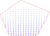
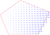
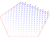
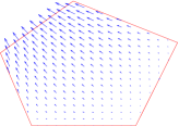
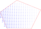
Figure 1. Basis $\{\mathbf{q}_{i}\}$ for $H(\mathrm{div})$ element on a random pentagon.

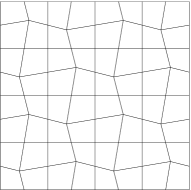
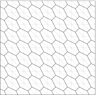
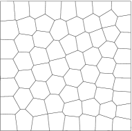
Figure 2. Meshes of size $8\times 8$. (1) A quadrilateral mesh. (2) A hexagonal mesh, with mostly hexagons and a few pentagons and quadrilaterals. It is generated as the dual mesh of an $8\times 8$ uniform triangular mesh, as shown in dotted lines. (3) Centroidal Voronoi tessellation consisting of $8\times 8$ cells (see [13] and references therein).

Consider the Poisson’s equation on $(0,1)\times(0,1)$ with Dirichlet boundary condition. We test this problem on three different types of meshes, as shown in Figure 2. Wachspress coordinates are used to define $\lambda_{i}$. The example problem is solved on a sequence of meshes, using the mixed finite element method with $\chi(\mathcal{M}\Lambda^{1}(T))$-$\mathbb{R}$ discretization. Denote by $\mathbf{p}$ and $u$ the exact flux and the exact primal solution, while by $\mathbf{p}_{h}$ and $u_{h}$ the corresponding numerical solutions. We first set the exact solution to be $u=\sin(\pi x)\sin(\pi y)$, which is smooth. Numerical results are reported in Tables 1-3, in which the ‘order’ is the value of $r$ in $O(h^{r})$ computed using the errors on two consecutive meshes. From the table we can see that $\|\mathbf{p}-\mathbf{p}_{h}\|_{L^{2}}$, $\|\mathrm{div}\mathbf{p}-\mathrm{div}\mathbf{p}_{h}\|_{L^{2}}$ and $\|u-u_{h}\|_{L^{2}}$ have at least $O(h)$ convergence, which agrees well with the theoretical prediction. We also point out that although the centroidal Voronoi tessellation in Figure 2 appears to contain very short edges, which may theoretically break the condition given in [19] for the assumption (3.4), the numerical results presented in Table 3 seem to be unaffected.

Table 1. Example problem with exact solution $u=\sin(\pi x)\sin(\pi y)$. Errors of the $\chi(\mathcal{M}\Lambda^{1}(T))$-$\mathbb{R}$ approximation on quadrilateral meshes as shown in Figure 2.

	$\|\mathbf{p}-\mathbf{p}_{h}\|_{L^{2}}$		$\|\mathrm{div}\mathbf{p}-\mathrm{div}\mathbf{p}_{h}\|_{L^{2}}$		$\|u-u_{h}\|_{L^{2}}$
Mesh Size	error	order	error	order	error	order
$4\times 4$	5.2843e-1		3.1580e+0		1.6184e-1
$8\times 8$	2.6040e-1	1.0210	1.6087e+0	0.9731	8.1764e-2	0.9850
$16\times 16$	1.2971e-1	1.0054	8.0813e-1	0.9932	4.0974e-2	0.9968
$32\times 32$	6.4810e-2	1.0010	4.0454e-1	0.9983	2.0498e-2	0.9992
$64\times 64$	3.2405e-2	1.0000	2.0233e-1	0.9996	1.0251e-2	0.9997
$128\times 128$	1.6204e-2	0.9999	1.0117e-1	0.9999	5.1255e-3	1.0000
$256\times 256$	8.1023e-3	0.9999	5.0587e-2	0.9999	2.5628e-3	1.0000
$512\times 512$	4.0513e-3	0.9999	2.5293e-2	1.0000	1.2814e-3	1.0000

Table 2. Example problem with exact solution $u=\sin(\pi x)\sin(\pi y)$. Errors of the $\chi(\mathcal{M}\Lambda^{1}(T))$-$\mathbb{R}$ approximation on hexagonal meshes as shown in Figure 2.

	$\|\mathbf{p}-\mathbf{p}_{h}\|_{L^{2}}$		$\|\mathrm{div}\mathbf{p}-\mathrm{div}\mathbf{p}_{h}\|_{L^{2}}$		$\|u-u_{h}\|_{L^{2}}$
Mesh Size	error	order	error	order	error	order
$4\times 4$	2.7502e-1		2.6008e+0		1.3488e-1
$8\times 8$	1.0994e-1	1.3228	1.4988e+0	0.7951	7.6665e-2	0.8150
$16\times 16$	4.5041e-2	1.2874	7.9379e-1	0.9170	4.0330e-2	0.9267
$32\times 32$	2.0013e-2	1.1703	4.0721e-1	0.9630	2.0646e-2	0.9660
$64\times 64$	9.4150e-3	1.0879	2.0608e-1	0.9826	1.0442e-2	0.9835
$128\times 128$	4.5673e-3	1.0436	1.0365e-1	0.9915	5.2510e-3	0.9917
$256\times 256$	2.2498e-3	1.0215	5.1973e-2	0.9959	2.6330e-3	0.9959
$512\times 512$	1.1166e-3	1.0107	2.6023e-2	0.9980	1.3184e-3	0.9979

Table 3. Example problem with exact solution $u=\sin(\pi x)\sin(\pi y)$. Errors of the $\chi(\mathcal{M}\Lambda^{1}(T))$-$\mathbb{R}$ approximation on centroidal Voronoi tessellations as shown in Figure 2.

	$\|\mathbf{p}-\mathbf{p}_{h}\|_{L^{2}}$		$\|\mathrm{div}\mathbf{p}-\mathrm{div}\mathbf{p}_{h}\|_{L^{2}}$		$\|u-u_{h}\|_{L^{2}}$
Mesh Size	error	order	error	order	error	order
$4\times 4$	4.5335e-1		3.1186e+0		1.6102e-1
$8\times 8$	1.8368e-1	1.3034	1.5915e+0	0.9705	8.1220e-2	0.9873
$16\times 16$	7.4684e-2	1.2983	7.7831e-1	1.0320	3.9513e-2	1.0395
$32\times 32$	2.9515e-2	1.3394	3.9116e-1	0.9926	1.9829e-2	0.9947
$64\times 64$	1.3361e-2	1.1434	1.9703e-1	0.9893	9.9831e-3	0.9901
$128\times 128$	6.3094e-3	1.0825	9.7955e-2	1.0082	4.9627e-3	1.0084
$256\times 256$	3.0048e-3	1.0702	4.8807e-2	1.0050	2.4726e-3	1.0051

It would be interesting to compare the numerical results on quadrilateral meshes given in Table 1, with the numerical results of the lowest order Raviart-Thomas element presented in [1]. The Raviart-Thomas element can be extended to convex quadrilaterals via the Piola transform associated to a bilinear isomorphism, but with a degeneration of approximation rate in $\|\mathrm{div}(\mathbf{p}-\mathbf{p}_{h})\|_{L^{2}}$ (see [1]). It is not hard to check that, on quadrilaterals that are not parallelograms, the space $\chi\left(\mathcal{M}\Lambda^{1}(T)\right)$ is indeed different from the polynomial-valued, lowest-order Raviart-Thomas element via Piola transform, because in this case $\chi\left(\mathcal{M}\Lambda^{1}(T)\right)$ consists of rational functions. Therefore, the $\chi\left(\mathcal{M}\Lambda^{1}(T)\right)$-$\mathbb{R}$ discretization will still provide optimal $O(h)$ convergence rate in $\|\mathrm{div}(\mathbf{p}-\mathbf{p}_{h})\|_{L^{2}}$, as shown in Table 1. In comparison, numerical results given in [1], using the lowest order Raviart-Thomas element via Piola transform, does not convergence in $\|\mathrm{div}\mathbf{p}-\mathrm{div}\mathbf{p}_{h}\|_{L^{2}}$ when the mesh consists of general quadrilaterals.

Table 4. Example problem with exact solution $u\in H^{3/2}$. Errors of the $\chi(\mathcal{M}\Lambda^{1}(T))$-$\mathbb{R}$ approximation on quadrilateral meshes as shown in Figure 2.

	$\|\mathbf{p}-\mathbf{p}_{h}\|_{L^{2}}$		$\|u-u_{h}\|_{L^{2}}$
Mesh Size	error	order	error	order
$4\times 4$	9.1202e-2		4.6653e-2
$8\times 8$	6.5317e-2	0.4816	2.3850e-2	0.9680
$16\times 16$	4.6480e-2	0.4909	1.2045e-2	0.9856
$32\times 32$	3.2970e-2	0.4955	6.0512e-3	0.9931
$64\times 64$	2.3350e-2	0.4977	3.0326e-3	0.9967
$128\times 128$	1.6524e-2	0.4989	1.5181e-3	0.9983
$256\times 256$	1.1689e-2	0.4994	7.5946e-4	0.9992
$512\times 512$	8.2669e-3	0.4997	3.7984e-4	0.9996

We also test a second example problem, under the same settings but with exact solution $u=\sqrt{\frac{1}{2}(\rho-x)}-\frac{1}{4}\rho^{2}$, where $\rho$ is the radius in polar coordinates. One can easily verify that $-\Delta u=1$ on $(0,1)\times(0,1)$, and moreover, $u\in H^{3/2}((0,1)^{2})$. Numerical results for the second example problem using the quadrilateral meshes are reported in Table 4. Note that $\|\mathrm{div}\mathbf{p}-\mathrm{div}\mathbf{p}_{h}\|_{L^{2}}$ is not included since for this test problem, one has $\mathrm{div}\mathbf{p}=\mathrm{div}\mathbf{p}_{h}\equiv-1$. From the table, we observe that $\|\mathbf{p}-\mathbf{p}_{h}\|_{L^{2}}$ is of approximately $O(h^{1/2})$, which is reasonable because $\mathbf{p}\in(H^{1/2})^{2}$, while $\|u-u_{h}\|_{L^{2}}\approx O(h)$ because $u$ is in $H^{3/2}$.

4. Construction in 3D

4.1. Definitions and properties

Let $T$ be a convex polyhedron satisfying Assumptions 1-2. Denote by $\mathbf{v}_{i}$, $i=1,\ldots,n$, the vertices of $T$. Then, for each pair of indices $\{i,j\}$, $1\leq i,j\leq n$, we have the Whitney $1$-form $W_{ij}$. Similarly, for each triplet of indices $\{i,j,k\}$, $1\leq i,j,k\leq n$, we have the Whitney $2$-form $W_{ijk}$. It is not hard to see that Whitney forms have the following properties:

$$W_{ii} =0,\qquad W_{ij}=-W_{ji},$$

$$W_{ijk} =0,\quad\textrm{if at least two of }i,j,k\textrm{ are identical},$$

$$W_{ijk} =W_{jki}=W_{kij}=-W_{ikj}=-W_{jki}=-W_{kji}.$$

Moreover, using the definition of Whitney forms, Equation (2.1) and elementary vector calculus identities, one has

(4.1) $$\mathrm{curl}\,W_{ij}=2\nabla\lambda_{i}\times\nabla\lambda_{j}=2\sum_{k=1}^{n}W_{ijk}.$$

We also state a result from [24]. Denote by $\boldsymbol{\tau}_{ij}=\mathbf{v}_{j}-\mathbf{v}_{i}$ for all $1\leq i,j\leq n$. For any constant vector $\mathbf{a}\in\mathbb{R}^{3}$, one has

(4.2) $$\frac{1}{2}\sum_{1\leq i,j\leq n}(\mathbf{a}\cdot\boldsymbol{\tau}_{ij})W_{ij} =\sum_{i<j}(\mathbf{a}\cdot\boldsymbol{\tau}_{ij})W_{ij}=\mathbf{a},$$

$$\frac{1}{2}\sum_{1\leq i,j\leq n}((\mathbf{a}\times\mathbf{v}_{i})\cdot\boldsymbol{\tau}_{ij})W_{ij} =\sum_{i<j}((\mathbf{a}\times\mathbf{v}_{i})\cdot\boldsymbol{\tau}_{ij})W_{ij}$$

$$=\sum_{i<j}((\mathbf{a}\times\mathbf{v}_{i})\cdot\mathbf{v}_{j})W_{ij}=\mathbf{a}\times\mathbf{x}.$$

The reason that Whitney forms are so important in the construction of $H(\mathrm{curl})$ and $H(\mathrm{div})$ spaces is that, they naturally satisfy certain conditions on edges/faces of $T$. Before summarizing these in lemmas, we first need to clarify the concept of ‘edges’. Denote by $e_{ij}$ the directed line segment pointing from $\mathbf{v}_{i}$ to $\mathbf{v}_{j}$, and by $|e_{ij}|$ its length . Notice that $e_{ij}$ may not be a natural edge of polyhedron $T$. Indeed, we classify all $e_{ij}$ into three disjoint categories:

1. $\mathcal{E}$ is the set of all $e_{ij}$ that coincides with a natural edge of $T$;

2. $\mathcal{E}_{F}$ is the set of all $e_{ij}$ lying on $\partial T$ but not in $\mathcal{E}$;

3. $\mathcal{E}_{I}$ is the set of all $e_{ij}$ in the interior of $T$, i.e., not lying on $\partial T$.

An illustration of these categories is given in Figure 3. We point out that each category actually contains both $e_{ij}$ and $e_{ji}$, for a given pair of indices $i$ and $j$. The union of all three categories covers all $e_{ij}$, for $1\leq i,j\leq n$. Notice that $\mathcal{E}_{F}$ and $\mathcal{E}_{I}$ can be empty for certain polyhedra. On each $e_{ij}$, denote by $\mathbf{t}_{ij}$ the unit tangential vector pointing from $\mathbf{v}_{i}$ to $\mathbf{v}_{j}$. We emphasize that only the $e_{ij}\in\mathcal{E}$ will be called an ‘edge’ of $T$, while the others are just called ‘directed line segments’.

Figure 3. Illustration of three categories: $e_{12}\in\mathcal{E}$, $e_{52}\in\mathcal{E}_{F}$, $e_{82}\in\mathcal{E}_{I}$.

Lemma 4.1.

Let $e_{kl}\in\mathcal{E}$. Then for all $1\leq i,j\leq n$, one has

$$W_{ij}\cdot\mathbf{t}_{kl}|_{e_{kl}}=\begin{cases}\frac{1}{|e_{ij}|}\quad&\textrm{if }e_{ij}=e_{kl},\\ -\frac{1}{|e_{ij}|}\quad&\textrm{if }e_{ij}=e_{lk},\\ 0&\textrm{otherwise}.\end{cases}$$

Proof.

The proof follows immediately from the definitions of $\lambda_{i}$, $W_{ij}$ and Assumption 1, which states that $\lambda_{i}$ is linear on all $e_{kl}\in\mathcal{E}$. ∎

Remark 4.2.

On $e_{kl}\in\mathcal{E}_{F}$ or $\mathcal{E}_{I}$, we do not have results similar to Lemma 4.1, since $\lambda_{i}$ may not even be linear on $e_{kl}$.

Next we define another important form on each $e_{ij}\in\mathcal{E}$. Denote by $\mathcal{F}_{ij}$ the set of two faces of polyhedron $T$ that share the edge $e_{ij}$, and by $\mathcal{V}_{ij}$ the set of all vertices on $\mathcal{F}_{ij}$. For a fixed index $1\leq i\leq n$, note that any $\boldsymbol{\tau}_{ik}$, for $e_{ik}\in\mathcal{E}_{I}$ can be written as a linear combination of all $\boldsymbol{\tau}_{ij}$, for $e_{ij}\in\mathcal{E}$. Such a linear combination is not uniquely defined if vertex $\mathbf{v}_{i}$ is connected to more than 3 edges of the polyhedron. Nevertheless, we can always fix a linear combination for each vertex $\mathbf{v}_{i}$, and denote this chosen one by

(4.3) $$\boldsymbol{\tau}_{ik}=\sum_{j,\,e_{ij}\in\mathcal{E}}C^{ik}_{ij}\boldsymbol{\tau}_{ij}.$$

Now, define

$$\tilde{W}_{ij} =W_{ij}+\frac{1}{2}\left(\sum_{\mathbf{v}_{k}\in\mathcal{V}_{ij},\,e_{ik}\in\mathcal{E}_{F}}W_{ik}-\sum_{\mathbf{v}_{k}\in\mathcal{V}_{ij},\,e_{jk}\in\mathcal{E}_{F}}W_{jk}\right)$$

$$\qquad+\frac{1}{2}\left(\sum_{k,\,e_{ik}\in\mathcal{E}_{I}}C^{ik}_{ij}W_{ik}-\sum_{k,\,e_{jk}\in\mathcal{E}_{I}}C^{jk}_{ji}W_{jk}\right).$$

In the above, one may view $W_{ij}+\frac{1}{2}\left(\sum_{\mathbf{v}_{k}\in\mathcal{V}_{ij},\,e_{ik}\in\mathcal{E}_{F}}W_{ik}-\sum_{\mathbf{v}_{k}\in\mathcal{V}_{ij},\,e_{jk}\in\mathcal{E}_{F}}W_{jk}\right)$ as the ‘surface’ component of $\tilde{W}_{ij}$ and $\frac{1}{2}\left(\sum_{k,\,e_{ik}\in\mathcal{E}_{I}}C^{ik}_{ij}W_{ik}-\sum_{k,\,e_{jk}\in\mathcal{E}_{I}}C^{jk}_{ji}W_{jk}\right)$ as the ‘interior’ component of $\tilde{W}_{ij}$. An illustration of the surface component of $\tilde{W}_{ij}$, which can also be written as $W_{ij}+\frac{1}{2}\left(\sum_{\mathbf{v}_{k}\in\mathcal{V}_{ij},\,e_{ik}\in\mathcal{E}_{F}}W_{ik}+\sum_{\mathbf{v}_{k}\in\mathcal{V}_{ij},\,e_{kj}\in\mathcal{E}_{F}}W_{kj}\right)$, is given in Figure 4. Note that if both faces sharing $e_{ij}$ are triangles, the surface component of $\tilde{W}_{ij}$ is just $W_{ij}$.

Figure 4. Illustration of surface component of $\tilde{W}_{ij}$ when $e_{ij}\in\mathcal{E}$ is shared by two faces of $T$ which are: (1) two triangles; (2) one triangle and one parallelogram; (3) two parallelograms. Here we conveniently use thick arrow to denote $W_{kl}$ and thin arrow to denote $\frac{1}{2}W_{kl}$ on any $e_{kl}$.

The vector function $\tilde{W}_{ij}$ has many nice properties. First, it is obvious that $\tilde{W}_{ij}=-\tilde{W}_{ji}$. Now, let us fix a direction for each edge of $T$. The collection of all edges in $\mathcal{E}$, with the prefixed direction, is denoted by $\mathcal{E}^{+}$. Similarly, one may denote the collection of all edges in $\mathcal{E}$ with direction opposite to the prefixed one as $\mathcal{E}^{-}$. The two sets $\mathcal{E}^{+}$ and $\mathcal{E}^{-}$ contain the same edges, but with opposite directions. For any two edges $e_{ij}$ and $e_{kl}$ in $\mathcal{E}^{+}$, denote by $\delta_{e_{ij},e_{kl}}$ the Kronecker delta whose value is $1$ if $e_{ij}=e_{kl}$ and $0$ otherwise. Then, we have the following lemmas:

Lemma 4.3.

The set $\{\tilde{W}_{ij},\textrm{ for }e_{ij}\in\mathcal{E}^{+}\}$ satisfy $\tilde{W}_{ij}\cdot\mathbf{t}_{kl}|_{e_{kl}}=\frac{1}{|e_{ij}|}\delta_{e_{ij},e_{kl}}$ for all $e_{kl}\in\mathcal{E}^{+}$, and hence is linearly independent.

Proof.

This follows immediately from the definition of $\tilde{W}_{ij}$, Lemma 4.1, and the fact that $\sum_{e_{ij}\in\mathcal{E}^{+}}c_{ij}\tilde{W}_{ij}=\mathbf{0}$ implies that $c_{kl}=|e_{kl}|\left(\sum_{e_{ij}\in\mathcal{E}^{+}}c_{ij}\tilde{W}_{ij}\right)\cdot\mathbf{t}_{kl}|_{e_{kl}}=0$ for all $e_{kl}\in\mathcal{E}^{+}$. ∎

Lemma 4.4.

It holds that $\mathcal{P}_{1}^{-}\Lambda^{1}(T)\subseteq span\{\tilde{W}_{ij},\textrm{ for }e_{ij}\in\mathcal{E}^{+}\}$.

Proof.

Let us first point out that $span\{\tilde{W}_{ij},\textrm{ for }e_{ij}\in\mathcal{E}^{+}\}=span\{\tilde{W}_{ij},\textrm{ for }e_{ij}\in\mathcal{E}\}$. By the definitions of $\tilde{W}_{ij}$ and $C^{ik}_{ij}$, Equation (4.2), Assumption 2, and the fact that $\mathbf{v}_{i}\times\boldsymbol{\tau}_{ij}=-\mathbf{v}_{j}\times\boldsymbol{\tau}_{ji}$, for any $\mathbf{a}\in\mathbb{R}^{3}$ one has

$$\sum_{e_{ij}\in\mathcal{E}} ((\mathbf{a}\times\mathbf{v}_{i})\cdot\boldsymbol{\tau}_{ij})\tilde{W}_{ij}=\sum_{e_{ij}\in\mathcal{E}}((\mathbf{a}\times\mathbf{v}_{i})\cdot\boldsymbol{\tau}_{ij})W_{ij}$$

$$+\frac{1}{2}\sum_{i=1}^{n}\sum_{k,\,e_{ik}\in\mathcal{E}_{F}}((\mathbf{a}\times\mathbf{v}_{i})\cdot\boldsymbol{\tau}_{ik})W_{ik}+\frac{1}{2}\sum_{j=1}^{n}\sum_{k,\,e_{jk}\in\mathcal{E}_{F}}((\mathbf{a}\times\mathbf{v}_{j})\cdot\boldsymbol{\tau}_{jk})W_{jk}$$

$$+\frac{1}{2}\sum_{i=1}^{n}\sum_{k,\,e_{ik}\in\mathcal{E}_{I}}((\mathbf{a}\times\mathbf{v}_{i})\cdot\boldsymbol{\tau}_{ik})W_{ik}+\frac{1}{2}\sum_{j=1}^{n}\sum_{k,\,e_{jk}\in\mathcal{E}_{I}}((\mathbf{a}\times\mathbf{v}_{j})\cdot\boldsymbol{\tau}_{jk})W_{jk}$$

$$=\sum_{i=1}^{n}\left(\sum_{k=1}^{n}((\mathbf{a}\times\mathbf{v}_{i})\cdot\boldsymbol{\tau}_{ik})W_{ik}\right)$$

$$=2\mathbf{a}\times\mathbf{x}.$$

This indicates that $\mathbf{a}\times\mathbf{x}\in span\{\tilde{W}_{ij},\textrm{ for }e_{ij}\in\mathcal{E}^{+}\}$. Similarly, one can prove that for any $\mathbf{b}\in\mathbb{R}^{3}$,

$$\sum_{e_{ij}\in\mathcal{E}}(\mathbf{b}\cdot\boldsymbol{\tau}_{ij})\tilde{W}_{ij}=2\mathbf{b}.$$

Recall that $\mathcal{P}_{1}^{-}\Lambda^{1}(T)=span\{\mathbf{a}\times\mathbf{x}+\mathbf{b},\textrm{ for all }\mathbf{a},\mathbf{b}\in\mathbb{R}^{3}\}$. This completes the proof of the lemma. ∎

Denote by $\mathcal{F}$ the set of all faces of $T$, and by $\mathbf{n}_{f}$ the unit outward normal vector on $f\in\mathcal{F}$ with respect to $T$. For each $f\in\mathcal{F}$, denote by $|f|$ its area and by $\partial f$ the oriented boundary of $f$ such that its orientation satisfies the right-hand rule with $\mathbf{n}_{f}$. If $e_{ij}$ lies on $\partial f$ and has the same direction as the orientation of $\partial f$, we say $e_{ij}\in\partial f$. If $e_{ij}$ lies on $\partial f$ and has the opposite direction as the orientation of $\partial f$, we say $e_{ij}\in-\partial f$.

Lemma 4.5.

Let $f\in\mathcal{F}$ and $e_{ij}\in\mathcal{E}$, then one has

$$\mathrm{curl}\tilde{W}_{ij}\cdot\mathbf{n}_{f}|_{f}=\begin{cases}\frac{1}{|f|}\quad&\textrm{if }e_{ij}\in\partial f,\\ -\frac{1}{|f|}\quad&\textrm{if }e_{ij}\in-\partial f,\\ 0\quad&\textrm{otherwise}.\end{cases}$$

Proof.

Notice that for any $f\in\mathcal{F}$ and $1\leq i,j\leq n$, by Equation (4.1), one has

$$\mathrm{curl}W_{ij}\cdot\mathbf{n}_{f}|_{f}=2(\nabla\lambda_{i}\times\nabla\lambda_{j})\cdot\mathbf{n}_{f}|_{f}=2(\nabla_{f}\lambda_{i}\times\nabla_{f}\lambda_{j})\cdot\mathbf{n}_{f}|_{f},$$

where $\nabla_{f}\lambda_{i}|_{f}$ denotes the tangential component of $\nabla\lambda_{i}$ on $f$. By Assumption 1, $\nabla_{f}\lambda_{i}|_{f}$ is non-zero only if $\mathbf{v}_{i}$ is a vertex on face $f$. It is then clear that $\mathrm{curl}W_{ij}\cdot\mathbf{n}_{f}|_{f}$ is non-zero only when both $\mathbf{v}_{i}$ and $\mathbf{v}_{j}$ are vertices of face $f$. Consequently, $\mathrm{curl}\tilde{W}_{ij}\cdot\mathbf{n}_{f}|_{f}$ is non-zero only when $e_{ij}\in\partial f$ or $-\partial f$.

For $f\in\mathcal{F}$, denote by $\mathcal{V}(f)$ the set of vertices on face $f$. Without loss of generality, assume $f$ lies on the $xy$-plane with outward normal $\mathbf{n}_{f}=[0,0,1]^{t}$, and denote by $\lambda_{k}^{(2)}$, for all $\mathbf{v}_{k}\in\mathcal{V}(f)$, the 2-dimensional barycentric coordinates on polygon $f$. By Assumption 1, the 3D coordinate $\lambda_{k}$, where $\mathbf{v}_{k}\in\mathcal{V}(f)$, degenerates to $\lambda^{(2)}_{k}$ on $f$. Consequently, $\nabla_{f}\lambda_{k}$ is equal to $\begin{bmatrix}\nabla^{(2)}\lambda^{(2)}_{k}\\ 0\end{bmatrix}$, where $\nabla^{(2)}$ stands for the 2-dimensional gradient on the $xy$-plane. Note we have for all $e_{kl}\in\partial f$ that

$$(\nabla_{f}\lambda_{k}\times\nabla_{f}\lambda_{l})\cdot\mathbf{n}_{f}|_{f}=\bigg{(}\begin{bmatrix}\nabla^{(2)}\lambda^{(2)}_{k}\\ 0\end{bmatrix}\times\begin{bmatrix}\nabla^{(2)}\lambda^{(2)}_{l}\\ 0\end{bmatrix}\bigg{)}\cdot\begin{bmatrix}0\\ 0\\ 1\end{bmatrix}=det[\nabla^{(2)}\lambda^{(2)}_{k}\;\nabla^{(2)}\lambda^{(2)}_{l}].$$

Consider the case $e_{ij}\in\partial f$. When $f$ is a triangle, it is clear that by Lemma 2.2

$$\mathrm{curl}\tilde{W}_{ij}\cdot\mathbf{n}_{f}|_{f}=\mathrm{curl}W_{ij}\cdot\mathbf{n}_{f}|_{f}=2(\nabla_{f}\lambda_{i}\times\nabla_{f}\lambda_{j})\cdot\mathbf{n}_{f}|_{f}=\frac{1}{|f|}.$$

When $f$ is a parallelogram, denote by $\mathbf{v}_{i}$, $\mathbf{v}_{j}$ $\mathbf{v}_{k}$ and $\mathbf{v}_{l}$ the vertices on $f$ such that $\partial f=\{e_{ij},e_{jk},e_{kl},e_{li}\}$. Then by the definition of $\tilde{W}_{ij}$ and Lemma 2.3,

$$(\mathrm{curl} \tilde{W}_{ij})\cdot\mathbf{n}_{f}|_{f}=\mathrm{curl}(W_{ij}+\frac{1}{2}W_{ik}+\frac{1}{2}W_{lj})\cdot\mathbf{n}_{f}|_{f}$$

$$=\mathrm{curl}\left(\frac{1}{2}(W_{ii}+W_{ij}+W_{ik}+W_{il})+\frac{1}{2}(W_{ij}+W_{jj}+W_{kj}+W_{lj})\right)\cdot\mathbf{n}_{f}|_{f}$$

$$\qquad-\frac{1}{2}\mathrm{curl}(W_{il}+W_{kj})\cdot\mathbf{n}_{f}|_{f}$$

$$=(\nabla_{f}\lambda_{i}\times\sum_{s\in\{i,j,k,l\}}\nabla_{f}\lambda_{s})\cdot\mathbf{n}_{f}|_{f}+\sum_{s\in\{i,j,k,l\}}\nabla_{f}\lambda_{s}\times\nabla_{f}\lambda_{j})\cdot\mathbf{n}_{f}|_{f}$$

$$\qquad+(\nabla_{f}\lambda_{l}\times\nabla_{f}\lambda_{i}+\nabla_{f}\lambda_{j}\times\nabla_{f}\lambda_{k})\cdot\mathbf{n}_{f}|_{f}$$

$$=0+0+\frac{1}{|f|}.$$

In the above we have used $W_{ii}=W_{jj}=0$ and $\sum_{s\in\{i,j,k,l\}}\nabla^{(2)}\lambda_{s}^{(2)}=\nabla^{(2)}1=\mathbf{0}$.

For $e_{ij}\in-\partial f$, one just needs to change the sign. This completes the proof of the lemma. ∎

Finally, on each $f\in\mathcal{F}$, define

$$\tilde{W}_{f}=\sum_{e_{ij}\in\partial f}\tilde{W}_{ij}.$$

By the definition and Lemma 4.5, we clearly have

(4.4) $$(\mathrm{curl}\,\tilde{W}_{f})\cdot\mathbf{n}_{f}|_{f}=\begin{cases}\frac{3}{|f|}\quad&\textrm{if }f\textrm{ is a triangle},\\ \frac{4}{|f|}\quad&\textrm{if }f\textrm{ is a parallelogram}.\end{cases}$$

Moreover, let $f^{\prime}\in\mathcal{F}$ be another face of $T$ that is different from $f$, then

(4.5) $$(\mathrm{curl}\,\tilde{W}_{f})\cdot\mathbf{n}_{f^{\prime}}|_{f^{\prime}}=\begin{cases}-\frac{1}{|f^{\prime}|}\quad&\textrm{if }f,f^{\prime}\textrm{ share an edge},\\ 0\quad&\textrm{if }f,f^{\prime}\textrm{ do not share edge}.\end{cases}$$

4.2. Discrete space and Basis function

Now we are able to construct spaces $\mathcal{M}\Lambda^{1}(T)$ and $\mathcal{M}\Lambda^{2}(T)$. It is very tempting to use $\tilde{W}_{ij}$, for all $e_{ij}\in\mathcal{E}^{+}$ as a set of basis for the $H(\mathrm{curl})$ finite element space $\mathcal{M}\Lambda^{1}(T)$. However, the biggest problem of doing so is that, we are not sure whether $\nabla\lambda_{i}\in span\{\tilde{W}_{ij},\textrm{ for }e_{ij}\in\mathcal{E}^{+}\}$ or not, and thus can not ensure the $\nabla\mathcal{M}\Lambda^{0}(T)\subset\mathcal{M}\Lambda^{1}(T)$ part in the sequence (1.5).

To ensure the exactness of sequence (1.5), similar to the 2D case, we will try

$$\mathcal{M}\Lambda^{1}(T) =\nabla\mathcal{M}\Lambda^{0}(T)\oplus\mathcal{H}=span\{\nabla\lambda_{i},\,i=1,\ldots,n\}\oplus\mathcal{H},$$

$$\mathcal{M}\Lambda^{2}(T) =\mathrm{curl}\,\mathcal{H}\oplus(\mathrm{div}^{\dagger})\mathbb{R},$$

where $\mathcal{H}$ is a space orthogonal to $span\{\nabla\lambda_{i},\,i=1,\ldots,n\}$. Again, in practice, it is very hard to construct orthogonal basis. Thus we relax the orthogonality requirement a little bit and replace $\oplus$ by $+$. Similar to (3.1), we construct the following:

(4.6) $$\mathcal{M}\Lambda^{1}(T) =span\{\nabla\lambda_{i},\,i=1,\ldots,n\}+span\{\tilde{W}_{f},\,f\in\mathcal{F}\},$$

(4.7) $$\mathcal{M}\Lambda^{2}(T) =\mathrm{curl}\,span\{\tilde{W}_{f},\,f\in\mathcal{F}\}+span\{\mathbf{x}-\mathbf{x}_{*}\}$$

$$=span\{\mathrm{curl}\,\tilde{W}_{f},\,f\in\mathcal{F}\}+span\{\mathbf{x}-\mathbf{x}_{*}\},$$

where $\mathbf{x}_{*}$ is a chosen point inside $T$. Of course this is just the construction. We still need to show that (1.5) is exact under this construction.

By definition, we have $\mathbb{R}\in\nabla\mathcal{M}\Lambda^{0}(T)$, $\nabla\mathcal{M}\Lambda^{0}(T)\subset\mathcal{M}\Lambda^{1}(T)$, $\mathrm{curl}\mathcal{M}\Lambda^{1}(T)\subset\mathcal{M}\Lambda^{2}(T)$ and $\mathrm{div}\mathcal{M}\Lambda^{2}(T)=\mathbb{R}$. Moreover, it is clear that $\mathrm{curl}\mathcal{M}\Lambda^{1}(T)\cap span\{\mathbf{x}-\mathbf{x}_{*}\}=\{\mathbf{0}\}$. These establish the exactness at the $\mathcal{M}\Lambda^{0}(T)$ and the $\mathcal{M}\Lambda^{2}(T)$ nodes. To show that (1.5) is exact at the $\mathcal{M}\Lambda^{1}(T)$ node, we only need to prove that no none-zero vector in $span\{\tilde{W}_{f},\,f\in\mathcal{F}\}$ is curl free. This can indeed be done by counting dimensions, i.e., we will prove that the dimensions of $\mathcal{M}\Lambda^{1}(T)$ and $\mathcal{M}\Lambda^{2}(T)$ are exactly $\#E$ and $\#F$, as indicated in (1.5). These dimensions are computed by explicitly constructing basis functions, as shown in the following two lemmas. We postpone the proof of these two lemmas to Appendix B.

Lemma 4.6.

There exists a computable basis $\{\mathbf{q}_{f},\textrm{ for }f\in\mathcal{F}\}$ for $\mathcal{M}\Lambda^{2}(T)$ defined in (4.7), such that on each $f^{\prime}\in\mathcal{F}$,

$$\mathbf{q}_{f}\cdot\mathbf{n}_{f^{\prime}}|_{f^{\prime}}=\begin{cases}1\quad&\textrm{if }f=f^{\prime},\\ 0&\textrm{otherwise}.\end{cases}$$

Therefore the dimension of $\mathcal{M}\Lambda^{2}(T)$ is equal to the number of faces of $T$.

Lemma 4.7.

There exists a computable basis $\{\mathbf{p}_{e},\textrm{ for }e\in\mathcal{E}^{+}\}$ for $\mathcal{M}\Lambda^{1}(T)$ defined in (4.6), such that on each $e^{\prime}\in\mathcal{E}^{+}$,

$$\mathbf{p}_{e}\cdot\mathbf{t}_{e^{\prime}}|_{e^{\prime}}=\begin{cases}1\quad&\textrm{if }e=e^{\prime},\\ 0&\textrm{otherwise}.\end{cases}$$

Therefore the dimension of $\mathcal{M}\Lambda^{1}(T)$ is equal to the number of edges of $T$.

Remark 4.8.

By the definitions of $\mathcal{M}\Lambda^{1}(T)$ and $\mathcal{M}\Lambda^{2}(T)$, lemmas 4.6-4.7, and by counting the dimensions, we know that (1.5) is an exact sequence.

Remark 4.9.

Lemma 4.6 indicates that for all $\mathbf{q}\in\mathcal{M}\Lambda^{2}(T)$, $\mathbf{q}\cdot\mathbf{n}$ is piecewise constant on the surface of $T$. Moreover, the normal components on faces of $T$ form a unisolvent set of degrees of freedom for $\mathcal{M}\Lambda^{2}(T)$, which allows one to build $H(\mathrm{div})$ conforming finite element space using $\mathcal{M}\Lambda^{2}(T)$.

Remark 4.10.

Similarly, Lemma 4.7 indicates that for all $\mathbf{q}\in\mathcal{M}\Lambda^{1}(T)$, $\mathbf{q}\cdot\mathbf{t}$ is piecewise constant on the skeleton of $T$, i.e., the collection of all edges in $\mathcal{E}$. Moreover, the tangential components on edges of $T$ form a unisolvent set of degrees of freedom for $\mathcal{M}\Lambda^{1}(T)$. However, this is not enough for building $H(\mathrm{curl})$ conforming finite element space, as $H(\mathrm{curl})$ conforming requires the tangential components on all faces, not only on edges, to be continuous across elements.

Next, we show that the basis $\mathbf{p}_{e}$ also provides tangential continuity across faces. For each $\mathbf{p}\in\mathcal{M}\Lambda^{1}(T)$, its value on a face $f\in\mathcal{F}$ can be split into two orthogonal parts

$$\mathbf{p}|_{f}=\mathcal{T}_{f}(\mathbf{p})+\mathcal{N}_{f}(\mathbf{p}),$$

where $\mathcal{T}_{f}(\mathbf{p})$ and $\mathcal{N}_{f}(\mathbf{p})$ are the vector projections of $\mathbf{p}|_{f}$ onto $f$ and its normal direction, respectively. We also denote by $\mathcal{T}_{\partial T}(\mathbf{p})$ the patching of $\mathcal{T}_{f}(\mathbf{p})$ over all $f\in\mathcal{F}$.

By the definition of $\mathcal{M}\Lambda^{1}(T)$ and $\tilde{W}_{f}$, it is clear that

$$\mathcal{M}\Lambda^{1}(T)\subseteq span\{\nabla\lambda_{i},\,i=1,\ldots,n\}+span\{\tilde{W}_{ij},\,e_{ij}\in\mathcal{E}\}.$$

But in general, we do not know whether $\nabla\lambda_{i}=-\sum_{j=1}^{n}W_{ij}$ is in $span\{\tilde{W}_{ij},\,e_{ij}\in\mathcal{E}\}$ or not. However, if only considering the tangential component, one has the following nice property:

Lemma 4.11.

Let $e_{ij}\in\mathcal{E}^{+}$ and $\mathbf{p}_{e_{ij}}$ be the basis function of $\mathcal{M}\Lambda^{1}(T)$ associated with edge $e_{ij}$. Then

$$\mathcal{T}_{\partial T}(\mathbf{p}_{e_{ij}})=\mathcal{T}_{\partial T}(|e_{ij}|\tilde{W}_{ij}).$$

Proof.

Clearly, $\mathcal{T}_{f}(W_{ij})$ is nonzero on $f$ only when both $\mathbf{v}_{i}$ and $\mathbf{v}_{j}$ lie on $f$. Note that Equation (3.3) is still true in 3D. Therefore, one has

$$\mathcal{T}_{\partial T}(\nabla\lambda_{i})=-\sum_{\begin{matrix}j\textrm{ such that}\\ e_{ij}\in\mathcal{E}\cup\mathcal{E}_{F}\end{matrix}}\mathcal{T}_{\partial T}(W_{ij})=-\sum_{\begin{matrix}j\textrm{ such that}\\ e_{ij}\in\mathcal{E}\end{matrix}}\mathcal{T}_{\partial T}(\tilde{W}_{ij}).$$

In the above we have used the definition of $\tilde{W}_{ij}$ to cancel out terms on $e_{kl}\in\mathcal{E}_{F}$ (if there exists any) that are not connected to vertex $\mathbf{v}_{i}$. Hence $\mathcal{T}_{\partial T}(\nabla\lambda_{i})\in span\{\mathcal{T}_{\partial T}(\tilde{W}_{ij}),\,e_{ij}\in\mathcal{E}\}$, which together with the definitions of $\tilde{W}_{f}$ and $\mathcal{M}\Lambda^{1}(T)$, further implies that

$$\mathcal{T}_{\partial T}(\mathcal{M}\Lambda^{1}(T)) \subseteq span\{\mathcal{T}_{\partial T}(\tilde{W}_{ij}),\,e_{ij}\in\mathcal{E}\}$$

$$=span\{\mathcal{T}_{\partial T}(\tilde{W}_{ij}),\,e_{ij}\in\mathcal{E}^{+}\}.$$

Therefore, by Lemma 4.3 and by comparing the tangential components on each edge, one must have $\mathcal{T}_{\partial T}(\mathbf{p}_{e_{ij}})=\mathcal{T}_{\partial T}(|e_{ij}|\tilde{W}_{ij})$ for all $e_{ij}\in\mathcal{E}^{+}$. This completes the proof of the lemma. ∎

Remark 4.12.

Lemma 4.11 tells us that the tangential component of each basis function $\mathbf{p}_{e_{ij}}$ on $\partial T$ is completely determined by the tangential component of $\tilde{W}_{ij}$. Let $T$ and $T^{\prime}$ be two polyhedra sharing a face $f$, and let $e_{ij}$ be an edge of the polygon $f$. Then, by the definition of $\tilde{W}_{ij}$ and Assumption 1, we know that $\mathbf{p}_{e_{ij}}$ has continuous tangential component across the face $f$. Thus one can build $H(\mathrm{curl})$ conforming finite element spaces using $\mathcal{M}\Lambda^{1}(T)$.

Remark 4.13.

If $\mathcal{E}_{I}=\emptyset$, then similar to the proof of Lemma 4.11, one can show $\nabla\lambda_{i}\in span\{\tilde{W}_{ij},\,e_{ij}\in\mathcal{E}\}$ and consequently $\mathbf{p}_{e_{ij}}=|e_{ij}|\tilde{W}_{ij}$. Examples of polyhedra with $\mathcal{E}_{I}=\emptyset$ include tetrahedra, pyramids and triangular prisms, but not rectangular boxes.

Next, we briefly show that $\mathcal{M}\Lambda^{k}(T)\subseteq\mathcal{W}\Lambda^{k}(T)$ for $k=1,2$. By Equation (3.3) and the definition of $\tilde{W}_{f}$, one immediately has $\mathcal{M}\Lambda^{1}(T)\subseteq\mathcal{W}\Lambda^{1}(T)$. Similarly, by Equation (4.1) and the definition of $\tilde{W}_{f}$, one gets $\mathrm{curl}\mathcal{M}\Lambda^{1}(T)\subseteq\mathcal{W}\Lambda^{2}(T)$. We also know from Equation (1.4) that $\mathbf{x}-\mathbf{x}_{*}\in\mathcal{W}\Lambda^{2}(T)$. Combining the above with the definition of $\mathcal{M}\Lambda^{2}(T)$ gives $\mathcal{M}\Lambda^{2}(T)\subseteq\mathcal{W}\Lambda^{2}(T)$.

Finally, to ensure the approximation property of $\mathcal{M}\Lambda^{k}(T)$, for $k=1,2$, we would like to have $\mathcal{P}_{1}^{-}\Lambda^{k}(T)\subseteq\mathcal{M}\Lambda^{k}(T)$. This is not easy to prove, and so far we do not even know whether it is in general true or not. Fortunately, we are able to prove this for two special types of polyhedra:

Type I:

Polyhedra with $\mathcal{E}_{I}=\emptyset$;

Type II:

Polyhedra with a center $\mathbf{x}_{c}$ such that for each vertex $\mathbf{v}_{i}$, $1\leq i\leq n$, one has

(4.8) $$(\mathbf{x}_{c}-\mathbf{v}_{i})\times\sum_{j,\,e_{ij}\in\mathcal{E}}\boldsymbol{\tau}_{ij}=0.$$

This is equivalent to say the barycenter of the point set $\{\mathbf{v}_{j},\textrm{ for all }e_{ij}\in\mathcal{E}\}$ lies in the line passing through $\mathbf{v}_{i}$ and $\mathbf{x}_{c}$.

The proof of the following Lemma will be given in Appendix C.

Lemma 4.14.

On Type I and II polyhedra, one has $\mathcal{P}_{1}^{-}\Lambda^{k}(T)\subseteq\mathcal{M}\Lambda^{k}(T)$ for $k=1,2$.

Remark 4.15.

Type I polyhedra include all tetrahedra, pyramids, and triangular prisms. Type II polyhedra include all parallelepipeds, all regular $n$-gon based bipyramids, the regular octahedron, the regular icosahedron, and some Catalan solids.

Remark 4.16.

From Lemma 4.14, we know that for Type I and II polyhedra, the definition of $\mathcal{M}\Lambda^{2}(T)$ is independent of the choice of $\mathbf{x}_{*}$, because $\mathbb{R}^{3}\subset\mathcal{P}_{1}^{-}\Lambda^{2}(T)$. But so far we do not know whether the definitions of $\mathcal{M}\Lambda^{1}(T)$ and $\mathcal{M}\Lambda^{2}(T)$ are independent of the linear combination given in Equation (4.3) or not.

Remark 4.17.

One may alternatively define an $H(\mathrm{curl})$ conforming finite element

$$\widetilde{\mathcal{M}\Lambda^{1}}(T)=span\{\tilde{W}_{ij},\textrm{ for }e_{ij}\in\mathcal{E}^{+}\},$$

which contains $\mathcal{P}_{1}^{-}\Lambda^{1}(T)$ according to Lemma 4.4 for all polyhedra satisfying Assumptions 1-2 (not restricted to Type I and II polyhedra). Moreover, by Remark 4.13, it is clear that $\widetilde{\mathcal{M}\Lambda^{1}}(T)=\mathcal{M}\Lambda^{1}(T)$ on Type I polyhedra. However, as mentioned in the beginning of this section, in general we do not know whether the alternative construction fits into a discrete exact sequence similar to (1.5) or not.

4.3. Examples

We show that our construction reproduces known $H(\mathrm{curl})$ and $H(\mathrm{div})$ elements on tetrahedra, rectangular boxes, pyramids, and triangular prisms. Then, we shall construct elements on a regular octahedron, which has never been done before.

In the construction, basis functions are computed according to the proof of lemmas 4.6 and 4.7, which is given in Appendix B. Wachspress coordinates are used to define $\lambda_{i}$. The computation can be done using any computer algebra system. The results are listed below:

1. On any tetrahedron, there exists a unique set of barycentric coordinates. One can indeed easily prove that $\mathcal{M}\Lambda^{k}(T)=\mathcal{W}\Lambda^{k}(T)=\mathcal{P}_{1}^{-}\Lambda^{k}(T)$ for $k=0,1,2$. No computation is needed.

2. On a rectangular box $(0,h_{1})\times(0,h_{2})\times(0,h_{3})$, by using the standard tensor product basis:

   $$\lambda_{1} =\frac{(h_{1}-x)(h_{2}-y)(h_{3}-z)}{h_{1}h_{2}h_{3}},\quad \lambda_{2} =\frac{x(h_{2}-y)(h_{3}-z)}{h_{1}h_{2}h_{3}},$$

   $$\lambda_{3} =\frac{xy(h_{3}-z)}{h_{1}h_{2}h_{3}},\quad \lambda_{4} =\frac{(h_{1}-x)y(h_{3}-z)}{h_{1}h_{2}h_{3}},$$

   $$\lambda_{5} =\frac{((h_{1}-x)(h_{2}-y)z}{h_{1}h_{2}h_{3}},\quad \lambda_{6} =\frac{x(h_{2}-y)z}{h_{1}h_{2}h_{3}},$$

   $$\lambda_{7} =\frac{xyz}{h_{1}h_{2}h_{3}},\quad \lambda_{8} =\frac{(h_{1}-x)yz}{h_{1}h_{2}h_{3}},$$

   Our construction gives

   $$\mathcal{M}\Lambda^{1}(T) =Q_{0,1,1}\times Q_{1,0,1}\times Q_{1,1,0},$$

   $$\mathcal{M}\Lambda^{2}(T) =Q_{1,0,0}\times Q_{0,1,0}\times Q_{0,0,1},$$

   where $Q_{I,J,K}=span\{x^{i}y^{j}z^{k},\,0\leq i\leq I,\,0\leq j\leq J,\,0\leq k\leq K\}$. These are identical to the lowest order Nédélec element defined in [36].

   Through the calculation, we also notice that on a rectangular box, the spaces $\mathcal{M}\Lambda^{1}(T)$ and $\mathcal{M}\Lambda^{2}(T)$ are much smaller than the spaces $\mathcal{W}\Lambda^{1}(T)$ and $\mathcal{W}\Lambda^{2}(T)$ constructed in [24]. For example, one can easily see that $W_{12}\in\mathcal{W}\Lambda^{1}(T)$ but not in $\mathcal{M}\Lambda^{1}(T)$. This indicates that there do exist redundant components in $\mathcal{W}\Lambda^{1}(T)$ and $\mathcal{W}\Lambda^{2}(T)$.

3. On a pyramid our construction is identical to the Whitney elements constructed by Grǎdinaru and Hiptmair in [26], if starting from the same $\mathcal{M}\Lambda^{0}(T)$ as in [26]. Since $\mathcal{E}_{I}=\emptyset$, one can use the simplification given in Remark 4.13, which coincides with the construction process in [26]. Thus we omit the details here.

4. On a triangular prism with base defined by $(0,0)$, $(1,0)$, $(0,1)$ and the vertical limits $0<z<1$, we use the following barycentric coordinates:

   $$\lambda_{1} =(1-x-y)(1-z),\qquad \lambda_{2} =x(1-z),\qquad \lambda_{3} =y(1-z),$$

   $$\lambda_{4} =(1-x-y)z,\qquad \lambda_{5} =xz,\qquad \lambda_{6} =yz.$$

   Our construction gives

   $$\mathcal{M}\Lambda^{1}(T) =\left\{\begin{bmatrix}(a_{1}-a_{3}y)+(a_{4}-a_{6}y)z\\ (a_{2}+a_{3}x)+(a_{5}+a_{6}x)z\\ a_{7}+a_{8}x+a_{9}z\end{bmatrix},\,a_{i}\in\mathbb{R}\textrm{ for }1\leq i\leq 9\right\},$$

   $$\mathcal{M}\Lambda^{2}(T) =\left\{\begin{bmatrix}a_{1}x+a_{2}\\ a_{1}y+a_{3}\\ a_{4}z+a_{5}\end{bmatrix},\,a_{i}\in\mathbb{R}\textrm{ for }1\leq i\leq 5\right\},$$

   which is identical to the lowest order elements on triangular prism constructed by Nédélec in [37].

5. Consider a regular octahedron, with vertices $\mathbf{v}_{1}:\>(0,0,-1)$, $\mathbf{v}_{2}:\>(1,0,0)$, $\mathbf{v}_{3}:\>(0,1,0)$, $\mathbf{v}_{4}:\>(-1,0,0)$, $\mathbf{v}_{5}:\>,(0,-1,0)$ and $\mathbf{v}_{6}:\>(0,0,1)$. The analytical form of basis functions would be to complicated to be enclosed in this paper, or to be analyzed directly. Here we draw the graph of two basis functions for $\mathcal{M}\Lambda^{2}(T)$ in Figure 5. In Matlab, we are also able to show that $\mathbb{R}^{3}\subset\mathcal{M}\Lambda^{2}(T)$ by computing certain linear combinations of the basis functions on a fine enough point grid, that reproduces constant vectors $[1,0,0]^{t}$, $[0,1,0]^{t}$ and $[0,0,1]^{t}$ on all grid points. This numerically verifies that $\mathbb{R}^{3}\subset\mathcal{M}\Lambda^{2}(T)$, which agrees with the theoretical result.

   

   

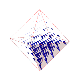
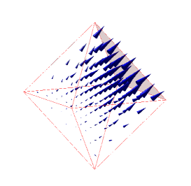
   Figure 5. Two basis functions for $\mathcal{M}\Lambda^{2}(T)$ on the regular octahedron. The normal component of the basis function is equal to $1$ on the shaded face and $0$ on all other faces.

We end this section with a brief discussion of elements on general hexahedra. Similar to the 2D quadrilateral case, the lowest order Raviart-Thomas element can be defined on hexahedra via Piola transform associated to a trilinear isomorphism, but requires asymptotically parallelepiped grid [6] in order to have good approximation rate. More results on the general hexahedral Nédélec-Raviart-Thomas elements can be found in the recent work [15] and references therein. In 3D, it is also possible for the image of the cube under a trilinear isomorphism to have non-planar faces. By working on the physical hexahedra directly, we can avoid this problem completely. However, a general hexahedron does not satisfy Assumption 2, and does not belong to either Type I or II. Nevertheless, a quick examination shows that $\widetilde{\mathcal{M}\Lambda^{1}}(T)$ from Remark 4.17 is still well-defined. Similar to the proof of Lemma 4.4 but requiring a more subtle treatment on $e_{kl}\in\mathcal{E}_{F}$, one can still show that $\widetilde{\mathcal{M}\Lambda^{1}}(T)$ contains $\mathcal{P}_{1}^{-}\Lambda^{1}(T)$ and consequently its curl contains $\mathbb{R}^{3}$. Therefore, $\widetilde{\mathcal{M}\Lambda^{1}}(T)$ may be used to build $H(\mathrm{curl})$ conforming finite element spaces on hexahedral meshes. In contrast, the situation for $\mathcal{M}\Lambda^{2}(T)$ is much more complicated, as we may not be able to keep the normal components on faces to be constants. Hence it remains a topic for future research.

Appendix A Adjacency matrices of a convex polyhedron

For a convex polyhedron $T$, we introduce a few integer-valued matrices related to the shape of the polyhedron. For convenience, let us temporarily index the edges in $\mathcal{E}^{+}$ by $e_{j}$, for $1\leq j\leq\#E$, and the faces in $\mathcal{F}$ by $f_{k}$, for $1\leq k\leq\#F$. Such kind of edge and face indices are only used in this section. In other parts of the paper, we do not index edges or faces of a polyhedron $T$ by a single integer, in order not to be confused with the integer indices for vertices.

Define matrices

$$A^{FtoE}:\>\mathbb{R}^{\#F}\to\mathbb{R}^{\#E},\quad \textrm{such that }A^{FtoE}_{ij}=\begin{cases}1\quad&\textrm{if }e_{i}\in\partial f_{j}\\ -1\quad&\textrm{if }e_{i}\in-\partial f_{j}\\ 0\quad&\textrm{otherwise}\end{cases},$$

$$A^{VtoE}:\>\mathbb{R}^{\#V}\to\mathbb{R}^{\#E},\quad \textrm{such that }A^{VtoE}_{ij}=\begin{cases}-1\quad&\textrm{if }e_{i}\textrm{ starts from }\mathbf{v}_{j}\\ 1\quad&\textrm{if }e_{i}\textrm{ ends at }\mathbf{v}_{j}\\ 0\quad&\textrm{otherwise}\end{cases}.$$

For each face $f_{i}\in\mathcal{F}$, denote by $n(f_{i})$ the number of edges in $f_{i}$. For each $\mathbf{v}_{i}\in\mathcal{V}$, denote by $n(\mathbf{v}_{i})$ the number of edges connected to $\mathbf{v}_{i}$. Define $M^{F}=(A^{FtoE})^{t}A^{FtoE}\in\mathbb{R}^{\#F\times\#F}$ and $M^{V}=(A^{VtoE})^{t}A^{VtoE}\in\mathbb{R}^{\#V\times\#V}$. It is not hard to see that the entries of $M^{F}$ and $M^{V}$ are

$$M^{F}_{ij}=\begin{cases}n(f_{i})\quad&\textrm{if }i=j,\\ -1\quad&\textrm{if }f_{i},\,f_{j}\textrm{ share an edge},\\ 0\quad&\textrm{otherwise},\end{cases}$$

and

$$M^{V}_{ij}=\begin{cases}n(\mathbf{v}_{i})\quad&\textrm{if }i=j,\\ -1\quad&\textrm{if }\mathbf{v}_{i},\,\mathbf{v}_{j}\textrm{ are connected by an edge},\\ 0\quad&\textrm{otherwise}.\end{cases}$$

To study the rank of $M^{F}$ and $M^{V}$, let us first state a well-known result:

Lemma A.1.

Let $M$ be an irreducible and (weakly) diagonally dominant square matrix, then $M$ either has full rank or a rank $1$ deficiency.

Proof.

For reader’s convenience, we provide a brief proof below. A square matrix is called irreducibly diagonally dominant if it is irreducible, weakly diagonally dominant but in at least one row is strictly diagonally dominant. Irreducibly diagonally dominant matrices are non-singular. Now, by changing only one entry in any chosen row of $M$, we can make it irreducibly diagonally dominant. Since changing one row of a matrix can at most modify its rank by $1$, therefore $M$ must either have full rank or a rank $1$ deficiency. ∎

Then, we have

Lemma A.2.

Matrix $M^{F}$ has rank $(\#F-1)$, and $Ker(M^{F})=span\{[1,1\ldots,1]^{t}\}$.

Proof.

By using the adjacency graph of the faces of $T$, it is not hard to see that $M^{F}$ is irreducible. Since the number of faces adjacent to each given face $f_{i}$ is equal to $n(f_{i})$, we know that $M^{F}$ is weakly diagonally dominant. By Lemma A.1, $M^{F}$ either has full rank or a rank $1$ deficiency. Indeed, $M$ has a rank $1$ deficiency, since one can explicitly compute that $[1,1\ldots,1]^{t}\in Ker(M^{F})$. This completes the proof of the lemma. ∎

Lemma A.3.

Matrix $M^{V}$ has rank $(\#V-1)$, and $Ker(M^{V})=span\{[1,1\ldots,1]^{t}\}$.

Proof.

The proof is similar to the proof of Lemma A.2. ∎

Finally, we mention another important property of the adjacency matrices:

Lemma A.4.

It holds that

(A.1) $$(A^{FtoE})^{t}A^{VtoE}=\mathbf{0}\quad\textrm{and}\quad(A^{VtoE})^{t}A^{FtoE}=\mathbf{0}.$$

Indeed, we have

$$Ker((A^{FtoE})^{t})=range(A^{VtoE})\quad\textrm{and}\quad Ker((A^{VtoE})^{t})=range(A^{FtoE}).$$

Proof.

By using the adjacency relations, it is elementary to prove (A.1). Consequently, one has

$$range(A^{VtoE})\subseteq Ker((A^{FtoE})^{t})\quad\textrm{and}\quad range(A^{FtoE})\subseteq Ker((A^{VtoE})^{t}).$$

Now, by lemmas A.2-A.3, we have $rank(A^{VtoE})=\#V-1$ and $rank(A^{FtoE})=\#F-1$. The lemma follows immediately from using the rank-nullity theorem and counting the dimensions. ∎

Appendix B Proof of lemmas 4.6 and 4.7

To prove Lemma 4.6, we first denote

$$\mathbf{q}_{f}=c_{f,0}(\mathbf{x}-\mathbf{x}_{*})+\sum_{\tilde{f}\in\mathcal{F}}c_{f,\tilde{f}}\mathrm{curl}\,\tilde{W}_{\tilde{f}},$$

and then show that there exists $\{c_{f,0},\,c_{f,\tilde{f}},\,\textrm{for }\tilde{f}\in\mathcal{F}\}$ such that $\mathbf{q}_{f}$ satisfies Lemma 4.6. Denote by $d_{f}$ the distance from $\mathbf{x}_{*}$ to face $f$, and by $|T_{f}|=\frac{1}{3}d_{f}|f|$ the volume of the pyramid with base $f$ and apex $\mathbf{x}_{*}$. For convenience, denote

$$\delta_{f,f^{\prime}}=\begin{cases}1\quad&\textrm{if }f=f^{\prime},\\ 0&\textrm{otherwise}.\end{cases}$$

For each $f^{\prime}\in\mathcal{F}$, denote by $\mathcal{F}(f^{\prime})$ the set of all faces in $\mathcal{F}$ that share an edge with $f^{\prime}$. Clearly, the number of faces in $\mathcal{F}(f^{\prime})$ is equal to the number of edges of polygon $f^{\prime}$, which is denote by $n(f^{\prime})$. Then, on each $f^{\prime}\in\mathcal{F}$, we want $\{c_{f,0},\,c_{f,\tilde{f}},\,\textrm{for }\tilde{f}\in\mathcal{F}\}$ to satisfy

(B.1) $$\delta_{f,f^{\prime}}=\mathbf{q}_{f}\cdot\mathbf{n}_{f^{\prime}}|_{f^{\prime}} =c_{f,0}(\mathbf{x}-\mathbf{x}_{*})\cdot\mathbf{n}_{f^{\prime}}|_{f^{\prime}}+\sum_{\tilde{f}\in\mathcal{F}}c_{f,\tilde{f}}\mathrm{curl}\,\tilde{W}_{\tilde{f}}\cdot\mathbf{n}_{f^{\prime}}|_{f^{\prime}}$$

$$=c_{f,0}d_{f^{\prime}}+c_{f,f^{\prime}}\frac{n(f^{\prime})}{|f^{\prime}|}-\sum_{\tilde{f}\in\mathcal{F}(f^{\prime})}\frac{c_{f,\tilde{f}}}{|f^{\prime}|},$$

where in the last step we have used equations (4.4)-(4.5). Multiplying both sides of (B.1) by $|f^{\prime}|$ and sum up over all $f^{\prime}\in\mathcal{F}$ gives

$$|f|=\sum_{f^{\prime}\in\mathcal{F}}c_{f,0}d_{f^{\prime}}|f^{\prime}|+0=3c_{f,0}|T|,$$

which implies

$$c_{f,0}=\frac{|f|}{3|T|}.$$

Now, Equation (B.1) can be rewritten into, for each $f^{\prime}\in\mathcal{F}$,

$$n(f^{\prime})c_{f,f^{\prime}}-\sum_{\tilde{f}\in\mathcal{F}(f^{\prime})}c_{f,\tilde{f}}=\delta_{f,f^{\prime}}|f^{\prime}|-\frac{|T_{f^{\prime}}|}{|T|}|f|.$$

This provides a linear system for solving $c_{f,\tilde{f}},\,\textrm{for all }\tilde{f}\in\mathcal{F}$, where the coefficient matrix is exactly $M^{F}$ defined in Appendix A. Note the right-hand side of the above linear system is obviously orthogonal to $Ker(M^{F})$, as

$$\sum_{f^{\prime}\in\mathcal{F}}\left(\delta_{f,f^{\prime}}|f^{\prime}|-\frac{|T_{f^{\prime}}|}{|T|}|f|\right)=0.$$

Therefore the linear system is solvable. This establishes the existence of $\mathbf{q}_{f}$ satisfying $\mathbf{q}_{f}\cdot\mathbf{n}_{f^{\prime}}|_{f^{\prime}}=\delta_{f,f^{\prime}}$. From the construction we also know that $\mathbf{q}_{f}$ is computable, with details given at the end of this section. Moreover, $\mathbf{q}_{f}$ is indeed uniquely defined since by setting $c_{f,\tilde{f}}=1$ for all $\tilde{f}\in\mathcal{F}$, i.e., by making the coefficients in $Ker(M^{F})$, one would get

$$\sum_{\tilde{f}\in\mathcal{F}}c_{f,\tilde{f}}\mathrm{curl}\,\tilde{W}_{\tilde{f}}=\mathrm{curl}\sum_{\tilde{f}\in\mathcal{F}}\tilde{W}_{\tilde{f}}=\mathrm{curl}\mathbf{0}=\mathbf{0},$$

where we have used the simple fact that $\sum_{f\in\mathcal{F}}\tilde{W}_{f}=\mathbf{0}$ according to the definition of $\tilde{W}_{f}$.

It is not hard to see that $\{\mathbf{q}_{f},\,\textrm{for }f\in\mathcal{F}\}$ is linearly independent. Again, by using $\sum_{f\in\mathcal{F}}\tilde{W}_{f}=\mathbf{0}$, we have

$$\dim\mathcal{M}\Lambda^{2}(T) \leq\dim\mathrm{curl}\left(span\{\tilde{W}_{f},\,f\in\mathcal{F}\}\right)+\dim span\{\mathbf{x}-\mathbf{x}_{*}\}$$

$$\leq\dim span\{\tilde{W}_{f},\,f\in\mathcal{F}\}+1$$

$$\leq(\#F-1)+1=\#F.$$

Combining the above, $\{\mathbf{q}_{f},\,\textrm{for }f\in\mathcal{F}\}$ must form a basis for $\mathcal{M}\Lambda^{2}(T)$ and consequently $\dim\mathcal{M}\Lambda^{2}(T)=\#F$. This completes the proof of Lemma 4.6.

Next we prove Lemma 4.7. The idea is similar to the proof of Lemma 4.6. We express

$$\mathbf{p}_{e}=\sum_{i=1}^{n}a_{e,i}\nabla\lambda_{i}+\sum_{f\in\mathcal{F}}b_{e,f}\tilde{W}_{f}.$$

Now, let $e^{\prime}\in\mathcal{E}^{+}$. Denote by $\mathbf{v}_{\alpha}$ and $\mathbf{v}_{\beta}$ the starting and ending vertices of $e^{\prime}$, and by $f_{l}$/$f_{r}$ the faces to the left/right of edge $e^{\prime}$, seeing from outside of $T$. Then, by Assumption 1, Lemma 4.3 and the definition of $\tilde{W}_{f}$, one has

$$\delta_{e,e^{\prime}} =\mathbf{p}_{e}\cdot\mathbf{t}_{e^{\prime}}|_{e^{\prime}}=\sum_{i=1}^{n}a_{e,i}\nabla\lambda_{i}\cdot\mathbf{t}_{e^{\prime}}|_{e^{\prime}}+\sum_{f\in\mathcal{F}}b_{e,f}\tilde{W}_{f}\cdot\mathbf{t}_{e^{\prime}}|_{e^{\prime}}$$

$$=\frac{-a_{e,\alpha}+a_{e,\beta}}{|e^{\prime}|}+\frac{b_{e,f_{l}}-b_{e,f_{r}}}{|e^{\prime}|},$$

which we further rewrite into

(B.2) $$-a_{e,\alpha}+a_{e,\beta}+b_{e,f_{l}}-b_{e,f_{r}}=\delta_{e,e^{\prime}}|e^{\prime}|.$$

The above equation holds on every $e^{\prime}\in\mathcal{E}^{+}$, and thus gives us a linear system with $\#E$ equations and $\#V+\#F=\#E+2$ unknowns. Denote by $A:\>\mathbb{R}^{\#E+2}\to\mathbb{R}^{\#E}$ the coefficient matrix of this linear system. It is not hard to see that, under proper ordering, one has

$$A=[A^{VtoE}\;A^{FtoE}],$$

where $A^{VtoE}$ and $A^{FtoE}$ are as defined in Appendix A.

By Lemma A.4, we have

$$A^{t}A=\begin{bmatrix}M^{V}&\mathbf{0}\\ \mathbf{0}&M^{F}\end{bmatrix}\in\mathbb{R}^{(\#E+2)\times(\#E+2)}.$$

Consequently, by lemmas A.2-A.3, we know that $rank(A)=rank(A^{t}A)=(\#V-1)+(\#F-1)=\#E$ and $Ker(A)$ is spanned by the following two vectors:

(B.3) $$[1,1,\ldots,1,0,0,\ldots,0]^{t},\quad\textrm{with }(\#V)\,1^{\prime}s\textrm{ and }(\#F)\,0^{\prime}s,$$

$$[0,0,\ldots,0,1,1,\ldots,1]^{t},\quad\textrm{with }(\#V)\,0^{\prime}s\textrm{ and }(\#F)\,1^{\prime}s.$$

Then, the linear system (B.2) is solvable. Moreover, we realize that $\mathbf{p}_{e}$ is indeed uniquely defined, as all coefficients in $Ker(A)$ only generate zero functions because $\sum_{i=1}^{n}\nabla\lambda_{i}=\mathbf{0}$ and $\sum_{f\in\mathcal{F}}\tilde{W}_{f}=\mathbf{0}$.

We can similarly show that $\{\mathbf{p}_{e},\,\textrm{for }e\in\mathcal{E}^{+}\}$ is linearly independent, and thus by counting dimensions, it form a basis for $\mathcal{M}\Lambda^{1}(T)$. This completes the proof of Lemma 4.7.

Finally, we briefly discuss how to compute the basis functions in practice. Using elementary linear algebra, it is not hard to see that:

1. To compute $\mathbf{q}_{f}$, one needs to solve a linear system $M^{F}\mathbf{u}=\mathbf{b}$, where $M^{F}\in\mathbb{R}^{\#F\times\#F}$ has a non-trivial kernel containing all constant vectors, and $\mathbf{b}\in Ker(M^{F})^{\perp}=Range(M^{F})$. Indeed, solving $M^{F}\mathbf{u}=\mathbf{b}$ is equivalent to solving a non-singular square system

   $$\begin{bmatrix}M^{F}&\mathbf{1}\\ \mathbf{1}^{t}&0\end{bmatrix}\begin{bmatrix}\mathbf{u}\\ 0\end{bmatrix}=\begin{bmatrix}\mathbf{b}\\ 0\end{bmatrix},$$

   where $\mathbf{1}$ denote a constant column vector with all entries equal to $1$.

2. To compute $\mathbf{q}_{e}$, one needs to solve a linear system $A\mathbf{u}=\mathbf{b}$, where $A=[A^{VtoE}\,A^{FtoE}]\in\mathbb{R}^{\#E\times(\#E+2)}$ has rank $\#E$ and kernel spanned by vectors in (B.3). Indeed, solving $A\mathbf{u}=\mathbf{b}$ is equivalent to solving a non-singular square system

   $$\begin{bmatrix}A^{VtoE}&A^{FtoE}\\ \mathbf{1}^{t}&\mathbf{0}^{t}\\ \mathbf{0}^{t}&\mathbf{1}^{t}\end{bmatrix}\mathbf{u}=\begin{bmatrix}\mathbf{b}\\ 0\\ 0\end{bmatrix}.$$

Appendix C Proof of Lemma 4.14

For Type I polyhedra, the proof is easy. By Remark 4.13, we have $\mathbf{p}_{e_{ij}}=|e_{ij}|\tilde{W}_{ij}$ on each $e_{ij}\in\mathcal{E}^{+}$. Thus by Lemma 4.4, one immediately gets $\mathcal{P}_{1}^{-}\Lambda^{1}(T)\subseteq\mathcal{M}\Lambda^{1}(T)$. This, together with the fact that $\mathrm{curl}(\mathbf{a}\times\mathbf{x})=2\mathbf{a}$ for all $\mathbf{a}\in\mathbb{R}^{3}$, implies that $\mathbb{R}^{3}\subset\mathcal{M}\Lambda^{2}(T)$. Finally, since $span\{\mathbf{x}-\mathbf{x}_{*}\}\subset\mathcal{M}\Lambda^{2}(T)$, we have $\mathcal{P}_{1}^{-}\Lambda^{2}(T)\subseteq\mathcal{M}\Lambda^{2}(T)$.

Now let us consider Type II polyhedra. From the proof of Lemma 4.4, one has

$$2\sum_{e_{ij}\in\mathcal{E}^{+}}((\mathbf{a}\times(\mathbf{v}_{i}-\mathbf{x}_{c}))\cdot\boldsymbol{\tau}_{ij})\tilde{W}_{ij}=\sum_{e_{ij}\in\mathcal{E}}((\mathbf{a}\times(\mathbf{v}_{i}-\mathbf{x}_{c}))\cdot\boldsymbol{\tau}_{ij})\tilde{W}_{ij}=2\mathbf{a}\times(\mathbf{x}-\mathbf{x}_{c}),$$

for all $\mathbf{a}\in\mathbb{R}^{3}$. If we can show that

(C.1) $$\sum_{e_{ij}\in\mathcal{E}^{+}}((\mathbf{a}\times(\mathbf{v}_{i}-\mathbf{x}_{c}))\cdot\boldsymbol{\tau}_{ij})\tilde{W}_{ij}=\sum_{f\in\mathcal{F}}C_{f}\tilde{W}_{f}\in\mathcal{M}\Lambda^{1}(T),$$

this together with the face that $\mathbb{R}^{3}\subset\nabla\mathcal{M}\Lambda^{0}(T)\subset\mathcal{M}\Lambda^{1}(T)$ will imply $\mathcal{P}_{1}^{-}\Lambda^{1}(T)\subseteq\mathcal{M}\Lambda^{1}(T)$. And consequently one will be able to prove that $\mathcal{P}_{1}^{-}\Lambda^{2}(T)\subseteq\mathcal{M}\Lambda^{2}(T)$. Next, we focus on prove the existence of a set of coefficients $\{C_{f},\textrm{ for }f\in\mathcal{F}\}$ that satisfies (C.1).

For each $e_{ij}\in\mathcal{E}^{+}$, denote by $f^{ij}_{l}$ and $f^{ij}_{r}$ the faces on the left and right side of $e_{ij}$ respectively, seeing from outside of $T$. Notice that the right-hand side of Equation (C.1) can further be written into $\sum_{e_{ij}\in\mathcal{E}^{+}}(C_{f^{ij}_{l}}-C_{f^{ij}_{r}})\tilde{W}_{ij}$. Thus it remains to prove that the system

(C.2) $$C_{f^{ij}_{l}}-C_{f^{ij}_{r}}=(\mathbf{a}\times(\mathbf{v}_{i}-\mathbf{x}_{c}))\cdot\boldsymbol{\tau}_{ij},\qquad\textrm{for all }e_{ij}\in\mathcal{E}^{+},$$

is solvable. The coefficient matrix of system (C.2) is exactly $A^{FtoE}$, as defined in Appendix A. Denote the right-hand side vector of system (C.2) by

$$\mathbf{b}=[(\mathbf{a}\times(\mathbf{v}_{i}-\mathbf{x}_{c}))\cdot\boldsymbol{\tau}_{ij}]_{e_{ij}\in\mathcal{E}^{+}}\in\mathbb{R}^{\#E}.$$

The linear system (C.2) is solvable only if

$$\mathbf{b}\in Range(A^{FtoE})=Ker((A^{FtoE})^{t})^{\perp}.$$

By Lemma A.4, we have $Ker((A^{FtoE})^{t})^{\perp}=range(A^{VtoE})^{\perp}=Ker((A^{VtoE})^{t})$. Therefore, System (C.2) is solvable as long as $(A^{VtoE})^{t}\mathbf{b}=\mathbf{0}$, which can be explicitly written as

(C.3) $$\sum_{j,\,e_{ij}\in\mathcal{E}^{+}}b_{ij}-\sum_{j,\,e_{ji}\in\mathcal{E}^{+}}b_{ji}=0,\qquad\textrm{for all }1\leq i\leq n,$$

where we conveniently denote by $b_{ij}$ the entry of vector $\mathbf{b}$ corresponding to $e_{ij}\in\mathcal{E}^{+}$. According to (C.2), $b_{ij}$ can be viewed as the jump of coefficient $C_{f}$ across the edge $e_{ij}$. Thus the constraints given by (C.3) are equivalent to say that, the summation of such jumps over all edges connecting to one given vertex should be $0$. By the definition of $\mathbf{b}$ and the fact that $\mathbf{v}_{i}\times\boldsymbol{\tau}_{ij}=\mathbf{v}_{j}\times\boldsymbol{\tau}_{ij}$, Equation (C.3) is equivalent to

$$\sum_{j,\,e_{ij}\in\mathcal{E}^{+}}(\mathbf{a}\times(\mathbf{v}_{i}-\mathbf{x}_{c}))\cdot\boldsymbol{\tau}_{ij}-\sum_{j,\,e_{ji}\in\mathcal{E}^{+}}(\mathbf{a}\times(\mathbf{v}_{j}-\mathbf{x}_{c}))\cdot\boldsymbol{\tau}_{ji}=\sum_{j,\,e_{ij}\in\mathcal{E}}(\mathbf{a}\times(\mathbf{v}_{i}-\mathbf{x}_{c}))\cdot\boldsymbol{\tau}_{ij}=0,$$

for all $1\leq i\leq n$, which is true on Type II polyhedra. In other words, we have shown that for Type II polyhedra, Equation (C.2) is solvable. This completes the proof of Lemma 4.14.

References

- [1] D. Arnold, D. Boffi, and R.S. Falk, Quadrilateral finite elements, SIAM J. Numer. Anal., 42 (2005), pp. 2429-2451.
- [2] D.N. Arnold, R.S. Falk and R. Winther, Finite element exterior calculus, homological techniques, and applications, Acta Numerica, (2006), pp. 1-155.
- [3] D.N. Arnold, R.S. Falk and R. Winther, Differential complexes and stability of finite element methods. I. The de Rham complex, Compatible Spatial Discretizations, The IMA Volumes in Mathematics and its Applications, Volume 142, pp. 23-46, Springer, New York, 2006.
- [4] D.N. Arnold, R.S. Falk and R. Winther, Geometric decompositions and local bases for spaces of finite element differential forms, Comput. Methods Appl. Mech. Engrg., 198 (2009), pp. 1660-1672.
- [5] D.N. Arnold, R.S. Falk and R. Winther, Finite element exterior calculus: from Hodge theory to numerical stability, Bull. Amer. Math. Soc. 47 (2010), pp. 281-354.
- [6] A. Bermúdez, P. Gamallo, M.R. Nogeiras and R. Rodríguez, Approximation properties of lowest-order hexahedral Raviart- Thomas elements, C. R. Acad. Sci. Paris, Ser. I, 340 (2005), pp. 687-692.
- [7] A. Bossavit, Whitney forms: a class of finite elements for three-dimensional computations in electromagnetism, IEE Proceedings A, 135 (1988), pp. 493-500.
- [8] A. Bossavit, A uniform rationale for Whitney forms on various supporting shapes, Math. & Comp. in Simulation, 80 (2010), pp. 1567-1577.
- [9] F. Brezzi and M. Fortin, Mixed and hybrid finite element methods, Springer, New York, 1991.
- [10] F. Brezzi, K. Lipnikov, and M. Shashkov, Convergence of the mimetic finite difference method for diffusion problems on polyhedral meshes, SIAM J. Numer. Anal., 43 (2005), pp. 1872-1896.
- [11] S.H. Christiansen, A construction of spaces of compatible differential forms on cellular complexes, Mathematical Models and Methods in Applied Sciences, 18 (2008), pp. 739-757.
- [12] P. Clément, Approximation by finite element functions using local regularization, RAIRO Analyse Numérique, 9 (1975), R-2, 77-84.
- [13] Q. Du, V. Faber, and M. Gunzburger, Centroidal Voronoi tessellations: Applications and algorithms, SIAM Rev., 41 (1999), pp. 637-676.
- [14] T. Euler, R. Schuhmann, and T. Weiland, Polygonal finite elements, IEEE Trans. Magnetics, 42 (2006), pp. 675-678.
- [15] R.S. Falk, P. Gatto, and P. Monk, Hexahedral and finite elements, ESAIM: M2AN, 45 (2011), pp. 115-143.
- [16] M.S. Floater, Mean value coordinates, Comp. Aided Geom. Design 20 (2003), pp. 19-27.
- [17] M.S. Floater, G. Kós, and M. Reimers, Mean value coordinates in 3D, Comp. Aided Geom. Design, 22 (2005), pp. 623-631.
- [18] M.S. Floater, K. Hormann, and G. Kós, A general construction of barycentric coordinates over convex polygons, Advances in Comp. Math., 24 (2006), pp. 311-331.
- [19] M.S. Floater, A. Gillette, and N. Sukumar, Gradient bounds for Wachspress coordinates on polytopes, SIAM J. Numer. Anal. 52 (2014), pp. 515-532.
- [20] M.S. Floater, Generalized barycentric coordinates and applications, Acta Numerica, (2015), doi:10.1017/S09624929.
- [21] A. Gillette and C. Bajaj, A generalization for stable mixed finite elements, Proceedings of the 14th ACM Symposium on Solid and Physical Modeling, pp. 41-50, 2010.
- [22] A. Gillette and C. Bajaj, Dual formulations of mixed finite element methods with applications, Comput. Aided Design, 43 (2011), pp. 1213-1221.
- [23] A. Gillette, A. Rand, and C. Bajaj, Error estimates for generalized barycentric coordinates, Adv. Comput. Math., 37 (2012), pp. 417-439.
- [24] A. Gillette, A. Rand, and C. Bajaj, Construction of scalar and vector finite element families on polygonal and polyhedral meshes, arXiv:1405.6978v1.
- [25] V. Grǎdinaru, Whitney elements on sparse grids, Dissertation, Universität Tübingen, 2002.
- [26] V. Grǎdinaru and R. Hiptmair, Whitney elements on pyramids, ETNA 8 (1999), pp. 154-168.
- [27] R. Herbin, Finite volume methods for diffusion convection equations on general meshes, in Finite volumes for complex applications, Problems and Perspectives, pp. 153-160, Hermes, 1996.
- [28] P. Joshi, M. Meyer, T. DeRose, B, Green, and T. Sanocki, Harmonic coordinates for character articulation, ACM Transactions on Graphics, 26 (2007), Article 71.
- [29] R. A. Klausen, A.F. Rasmussen, A.F. Stephansen, Velocity interpolation and streamline tracing on irregular geometries, Comput. Geosci., 16 (2012), pp. 261-276.
- [30] Y. Kuznetsov and S. Repin, Mixed finite element method on polygonal and polyhedral meshes, Numerical Mathematics and Advanced Applications, Proceedings of ENUMATH 2003, pp. 615-622, Springer-Verlag, Berlin Heidelberg, 2004.
- [31] Y. Kuznetsov, Mixed finite element methods on polyhedral meshes for diffusion equations, Partial Differential Equations: Modeling and Numerical Simulation, in Series Computational Methods in Applied Sciences, pp.27-41, Springer, Netherlands, 2008.
- [32] K. Lipnikov, G. Manzini, and M Shashkov, Mimetic finite difference method, J. Comp. Phys., 257 (2014), pp. 1163-1227.
- [33] G. Manzini, A. Russo and N. Sukumar, New perspectives on polygonal and polyhedral finite element methods, Math. Models Methods Appl. Sci., 24 (2014), pp. 1665-1699.
- [34] S. Martin, P. Kaufmann, M. Botsch, M. Wicke, and M. Gross, Polyhedral finite elements using harmonic basis functions, Computer Graphics Forum 27(5) [Proceedings SGP], 2008.
- [35] L. Mu, X. Wang, and Y. Wang, Shape regularity conditions for polygonal/polyhedral meshes, exemplified in a discontinuous Galerkin discretization, Numer. Meth. Part. Diff. Eq., 31 (2015), pp. 308-325.
- [36] J.C., Nédélec, Mixed finite element in , Numer. Math., 35 (1980), pp. 315-341.
- [37] J.C., Nédélec, A new family of mixed finite elements in , Numer. Math., 50 (1986), pp. 57-81.
- [38] A. Rand, A. Gillette and C. Bajaj, Interpolation error estimates for mean value coordinates over convex polygons, Adv. Comput. Math., 39 (2013), pp. 327-347.
- [39] R. Sibon, A vector identity for the Dirichlet tessellation, Mathematical Proceedings of the Cambridge Philosophical Society, 87 (1980), pp. 151-155.
- [40] N. Sukumar and A. Tabarraei, Conforming polygonal finite elements, Int. J. Numer. Meth. Engng., 61 (2004), pp. 2045-2066.
- [41] N. Sukumar and E.A., Malsch, Recent advances in the construction of polygonal finite element interpolants, Archives of Computational Methods in Engineering, 13 (2006), pp. 129-163.
- [42] C. Talischi, G.H. Paulino, and C. Le, Honeycomb Wachspress finite elements for structural topology optimization, Structural and Multidisciplinary Optimization, 37 (2009), pp. 569-583.
- [43] C. Talischi, G.H. Paulino, A. Pereira, and I.F.M. Menezes, Polygonal finite elements for topology optimization: A unifying paradigm, International Journal for Numerical Methods in Engineering, 82 (2010), pp. 671-698.
- [44] L. Beirão da Veiga, F. Brezzi, A. Cangiani, G. Manzini, L.D. Marini, and A. Russo, Basic principles of virtual element methods, Mathematical Models and Methods in Applied Sciences, 23 (2013), pp. 199-214.
- [45] E.L. Wachspress, A rational finite element basis, Academic Press, 1975.
- [46] E.L. Wachspress, Barycentric coordinates for polytopes, Comp. Aided Geom. Design, 61 (2011), pp. 3319-3321.
- [47] J. Wang and X. Ye, A weak Galerkin mixed finite element method for second order elliptic problems, Math. Comp., 83 (2014), pp. 2101-2126.
- [48] J. Warren, Barycentric coordinates for convex polytopes, Adv. in Comp. Math., 6 (1996), pp. 97-108.
- [49] J. Warren, On the uniqueness of barycentric coordinates, Topics in Algebraic Geometry and Geometric Modeling, Contemporary Mathematics VOL. 334 (2003), pp. 93-99.
- [50] H. Whitney, Geometric integration theory, Princeton University Press, Princeton, 1957.
- [51] M. Wicke, M. Botsch and M. Gross, A finite element method on convex polyhedra, Computer Graphics Forum 26(3), Proceedings Eurographics, 2007, pp. 255-364.