Non-equispaced B-spline wavelets
Version with detailed proofs

Abstract

This paper has three main contributions. The first is the construction of wavelet transforms from B-spline scaling functions defined on a grid of non-equispaced knots. The new construction extends the equispaced, biorthogonal, compactly supported Cohen-Daubechies-Feauveau wavelets. The new construction is based on the factorisation of wavelet transforms into lifting steps. The second and third contributions are new insights on how to use these and other wavelets in statistical applications. The second contribution is related to the bias of a wavelet representation. It is investigated how the fine scaling coefficients should be derived from the observations. In the context of equispaced data, it is common practice to simply take the observations as fine scale coefficients. It is argued in this paper that this is not acceptable for non-interpolating wavelets on non-equidistant data. Finally, the third contribution is the study of the variance in a non-orthogonal wavelet transform in a new framework, replacing the numerical condition as a measure for non-orthogonality. By controlling the variances of the reconstruction from the wavelet coefficients, the new framework allows us to design wavelet transforms on irregular point sets with a focus on their use for smoothing or other applications in statistics.

Keywords

B-spline; wavelet; Cohen-Daubechies-Feauveau; penalised splines; non-equispaced; non-equidistant; lifting

AMS classification

42C40; 65T60; 65D07; 41A15; 65D10

1 Introduction

Ever since the early days of wavelet research, spline wavelets have enjoyed special attention in the community. Spline wavelets combine the benefits from a sparse multiscale approach using wavelets and the well known properties of splines, including the closed form expressions, the numerous recursion relations, the polynomial based regularity of the basis functions (Unser, 1997).

Splines (de Boor, 2001), formally defined by the recursion as in (2) below, are piecewise polynomials of a certain degree, with continuity constraints in the knots that connect the polynomial pieces. The position of these knots and the degrees of the polynomial pieces are key parameters in the numerous methods in computer aided geometric design and computer graphics that are based on splines. Splines are also a popular tool in numerical analysis, for instance in interpolation. Compared to full polynomial interpolation, spline interpolation is far less sensitive to numerical instabilities that lead to oscillations. The good numerical condition is linked to the fact that any spline function can be decomposed into a basis of compactly supported piecewise polynomials, so-called B-splines. In statistics, the coefficients of the B-spline decomposition can be estimated in a nonparametric regression context. The estimator typically minimizes the residual sum of squares, penalized by the roughness of the regression curve (Green and Silverman, 1994; Eubank, 1999). The spline wavelet smoothing, as discussed in Section 5 of this paper, can be considered as an extension of these smoothing splines towards sparsity oriented penalties and corresponding nonlinear smoothing based on thresholding. While smoothing splines have their knots on the locations of the observations, P-splines (Ruppert et al., 2003) allow a flexible choice of knots. An important advantage of any spline, whether it be an interpolating, smoothing or P-spline, is that it is known by an explicit expression. The main merit of a closed-form expression is that all information about the smoothness of the function, typically expressed by the Lipschitz regularity, is readily available for use in smoothing algorithms. The spline wavelets on irregular knots constructed in this paper are splines, and thus share this benefit. This is in contrast to most other wavelets, especially those on irregular point sets. The smoothness of these wavelets depends on the limit of an infinitely iterated refinement or subdivision scheme (Daubechies et al., 1999b), which can be hard to analyse, even for straightforward refinement schemes such as for Deslauries-Dubuc interpolating wavelets (Deslauriers and Dubuc, 1987, 1989; Donoho and Yu, 1999; Sweldens and Schröder, 1996).

The combination of splines and wavelets is, however, not trivial. One of the problems is that splines do not provide a naturally orthogonal basis. On the other hand, orthogonality is much appreciated in wavelet theory, because wavelet transforms operate scale after scale. In the inverse transform, i.e., in the reconstruction of a function from its wavelet coefficients, this scale to scale process amounts to the refinement or subdivision, mentioned above. Although the smoothness of the reconstruction in a spline basis does not depend on this refinement scheme, other properties do. These properties include the numerical condition of the transform as well as the bias and the variance in statistical estimation. The assumption of orthogonality facilitates the analysis of these properties throughout the subdivision scheme. Initial spline wavelet constructions were orthogonal (Battle, 1987; Lemarié, 1988). The price to pay for the orthogonality was that the basis functions did not have a compact support, and related to this, that transformation matrices were full, not sparse, matrices.

The condition of orthogonality can be relaxed if the basis functions within one scale are allowed to be non-orthogonal, while the wavelets at different scales are still kept orthogonal (Chui and Wang, 1992; Unser et al., 1992, 1993). This construction leads to a semi-orthogonal spline basis. Since the non-orthogonality occurs only within each scale, this has little impact on the asymptotic analysis of the refinement process. Moreover, semi-orthogonal wavelet bases can be constructed from non-orthogonal spline bases, such as B-splines. The B-splines and the resulting wavelets have compact support. As a consequence, the reconstruction of data from a decomposition in these bases uses a sparse matrix. Sparse matrices and compact supports lead to faster algorithms, but also contribute to better control over manipulations on the wavelet coefficients. A manipulation of a coefficient, such as a thresholding or shrinkage operation, has only a local effect.

Unfortunately, the forward transform of observations into the semi-orthogonal wavelet basis still requires the application of a full, non-sparse, matrix. This is because in general the inverse of a sparse matrix is not sparse. Sparse inverses are possible in a wide range of fast wavelet transforms, but the combination of the semi-orthogonality and the spline properties cannot be obtained within a sparse forward transform. As a consequence, every fine scale observation has at least some contribution to each wavelet coefficient. It would be better if not only a wavelet coefficient had local impact on the reconstruction of the observations but also, at the same time, the coefficient got its value from a limited number of observations. The latter, dual, form of compact support is possible in the framework of bi-orthogonal spline wavelets. The construction by Cohen, Daubechies, and Feauveau (1992) of a multiresolution analysis starting from B-splines has led to non-orthogonal wavelets with sparse decomposition and reconstruction matrices.

The Cohen-Daubechies-Feauveau wavelets are defined on equispaced knots. This is because the classical multiresolution theory starts from scaling bases whose basis functions are all dilations and translations of a single father function. This construction is not possible on irregular knots. B-splines, on the other hand, are easily defined on non-equispaced knots. This paper extends the construction by Cohen, Daubechies and Feauveau towards these non-equispaced B-splines. For the construction of wavelet transforms on non-equispaced knots, sometimes termed second generation wavelets (Daubechies et al., 1999a; Sweldens, 1998), this paper adopts the lifting scheme (Sweldens, 1996). The lifting scheme provides for every refinement operation in a wavelet transform a factorisation into simple steps within the scale of that refinement. The key contribution of this paper is to identify the lifting steps that are necessary in the factorisation of a B-spline refinement on non-equidistant knots.

Section 2 summarizes results from the literature that are necessary for the main contribution in Section 3.1. First, Section 2.1 defines the notion of multiscale grids. Then, Section 2.2 gives a definition of B-splines together with their properties for further use. Section 2.3 proposes to use a refinement equation as a definition for B-splines. In order to fill in coefficients in the equation, it needs to be factored into elementary operations. The result is a slight generalisation of the well known factorisation of equidistant wavelet transforms (Daubechies and Sweldens, 1998). Finally, Section 3.3 further investigates the role of the factorisation in wavelet transforms. The main contribution in Section 3.1 fills in the lifting steps that constitute a B-spline refinement. Section 3.4 gives an expression for all possible wavelets that fit within the B-spline refinement scheme. The first part of this paper, about the construction of non-equispaced B-spline wavelets is concluded by the short Section 3.5 on the non-decimated B-spline wavelet transform.

Other work on lifting for spline or B-spline wavelets, such as (Bertram, 2004; Chern, 1999; Fahmy, 2008; Li et al., 2005; Prestin and Quak, 2005; Xiang et al., 2007) is situated on equidistant knots or is focused on specific cases, such as Powell-Sabin spline wavelets (Vanraes et al., 2004). B-spline wavelets on non-equispaced knots have been studied for specific applications and with particular lifting schemes (Pan and Yao, 2009; Lyche et al., 2001). It should be noted that B-splines on non-equispaced knots are often termed non-uniform B-splines. This term is avoided in this paper, as in statistical sense, a uniform set of knots could be interpreted as a set of random, uniformly distributed knots, which are of course almost surely non-equidistant.

The second part of the paper consists of the Sections 4 and 5. It concentrates on the use of the B-spline wavelets from the first part in statistics. In statistical applications, B-spline wavelets are used, for instance, in a soft threshold scheme for noise reduction. Given that a soft threshold comes from an $\ell_{1}$ regularised least squares approximation of the input, this application is an example of a penalised spline method. The discussions in Sections 4 and 5 are quite general, and therefore applicable to other non-equispaced wavelets as well.

The discussion in Section 4 is related to the bias in a B-spline wavelet smoothing. It investigates how to proceed from observations to fine scaling coefficients. It is argued that in a situation with non-equispaced data, this step should be taken with care, in order to avoid to commit what some authors call the “wavelet crime” (Strang and Nguyen, 1996).

While Section 4 deals with bias, Section 5 is about the variance in a second generation wavelet transform. Assuming that the observations are independent, the variance of the transformed data is best understood if the transform is orthogonal. As the construction by Cohen, Daubechies and Feauveau, extended in this paper towards non-equidistant knots, has somehow less attention for orthogonality, this may cause major problems with estimators suffering from large variance effects (Vanraes et al., 2002; Van Aerschot et al., 2006; Jansen et al., 2009). Although the large variance is due to the transform being non-orthogonal, the classical numerical condition number is not a satisfactory quantification of the statistical problem. Therefore this paper proposes a multiscale variance propagation number, based on the singular values of the linear projection onto the coarse scale B-spline basis. From there, an alternative B-spline wavelet transform is developed. The alternative is closely related to the Cohen-Daubechies-Feauveau construction, but it keeps the variance propagation under control.

2 B-splines and multiresolution

This section reviews definitions and well established results on B-splines, multiscale representations and the lifting scheme.

2.1 Multilevel grids

Let $K_{n}=\{x_{k}|k=0,\ldots,n-1\}$ be a set of knots on which we will define B-splines. B-splines of order $\widetilde{p}$ are basis functions spanning all piecewise polynomials of degree $\widetilde{p}-1$ with continuous $\widetilde{p}-2$ derivatives in the knots. In this paper, the B-spline basis will be constructed through a process known as refinement or subdivision. For this process to work, we first have to define coarse scale versions of the grid of knots. We thus identify the input set of knots as the fine scale grid, formalised as $x_{J,k}=x_{k}$. The index $J$ refers to the highest or finest scale. From there, we define grids $\{x_{j,k}|k=0,\ldots,n_{j}-1\}$ at coarser scales $j$, where $j=L,L+1,\ldots,J-1$, $L$ being the lowest or coarsest scale. Obviously $n_{j}<n$ stands for the number of points at scale $j$. Denoting $\Delta_{j,k}=x_{j,k+1}-x_{j,k}$, and $\Delta_{j}=\sup_{k=0,\ldots,n_{j}-2}\Delta_{j,k}$, we call the grid at scale $j$ regular if $\Delta_{j,k}$ does not depend on $k$, i.e., $\Delta_{j,k}=\Delta_{j}$. The focus in this paper lies on irregular grids.

Definition 1

(multilevel grid) The sequence of grids constitutes a multilevel grid if the following conditions are met:

1. The sequence $n_{j}$ is strictly increasing.

2. There exist constants $R\in\mathbbm{R}$ and $\beta>0$ so that maximum gap at scale $j$ is bounded as follows

   $$\Delta_{j}\leq Rn_{j}^{-\beta}.$$ (1)

Condition (1) is a slightly stricter version of the definition adopted in (Daubechies et al., 2001), where in the context of binary or dyadic refinement, i.e., $n_{j}=2^{j}$, it is imposed that $\sum_{j=L}^{\infty}\Delta_{j}<\infty$. The condition can be understood by considering a sequence of functions $x_{j}:[0,1]\to\mathbbm{R}:u\mapsto x_{j}(u)$ for which $x_{j,k}=x_{j}(k/(n_{j}-1))$. The divided differences of $x_{j}(u)$ in the knots $k/(n_{j}-1)$ are then $\Delta_{j,k}(n_{j}-1)$. The divided differences must not or at most very slowly converge to a locally infinite derivative, in order not to leave any coarse scale gaps in a grid at fine scale.

A multilevel grid is nested if $x_{j+1,k}\in\{x_{j,k}|k=0,\ldots,n_{j}-1\}.$ In particular, the multilevel grid is two-nested if at each level, the grid is a binary refinement of the previous, coarser level, that is, if $x_{j+1,2k}=x_{j,k}$. This paper works with two-nested multilevel grids only.

2.2 B-splines at a fixed scale

Throughout this paper, $\varphi_{j,k}^{\left[\widetilde{p}\right]}(x)$ will stand for the B-spline of order $\widetilde{p}$ defined on the knots $x_{j,i}$. There exist several recursion expressions for the construction of B-splines. This paper will use the following formula (Qu and Gregory, 1992; Daubechies et al., 2001, page 497) as definition.

Definition 2

(B-splines) The B-splines of order 1 defined on the knots $x_{j,i}$ are the characteristic functions $\varphi_{j,k}^{\left[0\right]}(x)=\chi_{j,k}(x)$, where $\chi_{j,k}(x)=1\Leftrightarrow x\in[x_{j,k},x_{j,k+1})$ and $\chi_{j,k}(x)=0$ otherwise. B-splines of order 1 are also known as B-splines of degree 0.

B-splines of order $\widetilde{p}$, i.e., degree $\widetilde{p}-1$, for $\widetilde{p}>0$, are defined recursively as

$$\varphi_{j,k}^{\left[\widetilde{p}\right]}(x) = {x-x_{j,k-\left\lfloor\widetilde{p}/2\right\rfloor}\over x_{j,k+\left\lceil\widetilde{p}/2\right\rceil-1}-x_{j,k-\left\lfloor\widetilde{p}/2\right\rfloor}}\varphi_{j,k-1+\mathrm{rem}(\widetilde{p}/2)}^{\left[\widetilde{p}-1\right]}(x)$$ (2)

$$+ {x_{j,k+\left\lceil\widetilde{p}/2\right\rceil}-x\over x_{j,k+\left\lceil\widetilde{p}/2\right\rceil}-x_{j,k-\left\lfloor\widetilde{p}/2\right\rfloor+1}}\varphi_{j,k+\mathrm{rem}(\widetilde{p}/2)}^{\left[\widetilde{p}-1\right]}(x).$$

In this equation $\mathrm{rem}(p/q)=p-q\left\lfloor p/q\right\rfloor$ denotes the remainder from an integer division.

Later on in this paper, the construction through recursion will be replaced by a construction through refinement. On a finite set of knots, i.e., when $k\in\{0,\ldots,n_{j}-1\}$, both constructions are equivalent if we follow the convention in (2) that the left and right end points are multiple knots. More precisely, whenever a knot index in (2) is outside $\{0,\ldots,n_{j}-1\}$, then we take $x_{j,l}=x_{j,0}$ for $l<0$ and $x_{j,r}=x_{j,n_{j}-1}$ for $r>n_{j}-1$. Definition 2 associates with every knot $x_{j,k}$ a B-spline function $\varphi_{j,k}^{\left[\widetilde{p}\right]}(x)$. The function turns out to be centered around the corresponding knot, as can be seen from the following result.

Theorem 1

(piecewise polynomials on bounded intervals) For $k\in\{\left\lfloor\widetilde{p}/2\right\rfloor,\ldots,n-1-\left\lceil\widetilde{p}/2\right\rceil\}$ the function $\varphi_{j,k}^{\left[\widetilde{p}\right]}(x)$ is zero outside the interval $[x_{j,l_{k}},x_{j,r_{k}})$, where $l_{k}=k-\left\lfloor\widetilde{p}/2\right\rfloor$ and $r_{k}=k+\left\lceil\widetilde{p}/2\right\rceil$. Inside this interval, $\varphi_{j,k}^{\left[\widetilde{p}\right]}(x)$ is a polynomial of degree $\widetilde{p}-1$ between two knots $x_{j,k}$ and $x_{j,k+1}$, while in the knots, the function and its first $\widetilde{p}-2$ derivatives are continuous.

The proof follows by induction, using Definition 2.

Theorem 1 should be amended for functions $\varphi_{j,k}^{\left[\widetilde{p}\right]}$ near the boundaries, i.e., for $k$ close to 0 or $n_{j}-1$. The specification is postponed to the moment where the functions have been redefined using refinement instead of recursion. We first concentrate on the interior interval, defined by

$$I_{j}=\{x\in[x_{j,0},x_{j,n_{j}-1})|\forall k=0,\ldots,n_{j}-1:\varphi_{j,k}^{\left[\widetilde{p}\right]}(x)\neq 0\Rightarrow l_{k}\geq 0\mbox{ and }r_{k}\leq n_{j}-1\},$$ (3)

with $l_{k}$ and $r_{k}$ as defined in Theorem 1. It is straightforward to check that

$$I_{j}=\left[x_{j,\widetilde{p}-1},x_{j,n_{j}-\widetilde{p}}\right].$$ (4)

From Theorem 1, it is obvious that the set of B-splines $\left\{\varphi_{j,k}^{\left[\widetilde{p}\right]}\right\}$ generates piecewise polynomials. Conversely, it can be verified that any piecewise polynomial on the interior interval $I_{j}$ can be decomposed as a linear combination of B-splines.

Theorem 2

(B-spline basis) Let $f_{j}(x)$ be a function which is polynomial on each interval $[x_{j,k},x_{j,k+1})$ for which $\{x_{j,k},x_{j,k+1}\}\subset I_{j}$ and which has $p-2$ continuous derivatives in the knots $x_{j,k}\in I_{j}$. Then there exist constants $a_{j,k}$ so that for all $x\in I_{j}$,

$$f_{j}(x)=\sum_{k=\left\lfloor\widetilde{p}/2\right\rfloor}^{n_{j}-1-\left\lceil\widetilde{p}/2\right\rceil}a_{j,k}\,\varphi_{j,k}^{\left[\widetilde{p}\right]}(x)$$ (5)

Proof. See Appendix B.1.

Remark 1

Most references in literature would adopt the symbol $N_{j,k}^{\left[\widetilde{p}\right]}(x)$ for a shifted version of this basis, namely

$$\varphi_{j,k}^{\left[\widetilde{p}\right]}(x)=N_{j,k-\left\lfloor\widetilde{p}/2\right\rfloor}^{\left[\widetilde{p}\right]}(x).$$

The notation with $N_{j,k}^{\left[\widetilde{p}\right]}(x)$ leads to more elegant expressions for the recursion of B-splines, but it does not correspond to the common practice in wavelet literature where a basis function $\varphi_{j,k}(x)$ is centered around the point $x_{j,k}$.

The forthcoming discussions will use expressions for the derivatives of spline functions.

Lemma 1

The derivative of a B-spline is given by

$${d\over dx}\varphi_{j,k}^{\left[\widetilde{p}\right]}(x)=(\widetilde{p}-1)\left[{\varphi_{j,k-1+\mathrm{rem}(\widetilde{p}/2)}^{\left[\widetilde{p}-1\right]}(x)\over x_{j,k+\left\lceil\widetilde{p}/2\right\rceil-1}-x_{j,k-\left\lfloor\widetilde{p}/2\right\rfloor}}-{\varphi_{j,k+\mathrm{rem}(\widetilde{p}/2)}^{\left[\widetilde{p}-1\right]}(x)\over x_{j,k+\left\lceil\widetilde{p}/2\right\rceil}-x_{j,k-\left\lfloor\widetilde{p}/2\right\rfloor+1}}\right].$$ (6)

Lemma 6 can be proven by induction on $\widetilde{p}$. The computations are facilitated by working on the shifted index in $N_{j,k}^{\left[\widetilde{p}\right]}(x)$.

As a consequence of Lemma 6, a linear combination of the B-splines

$$f_{j}(x)=\sum_{k\in\mathbbm{Z}}s_{j,k}^{\left[\widetilde{p}\right]}\varphi_{j,k}^{\left[\widetilde{p}\right]}(x),$$ (7)

has a derivative equal to

$$f_{j}^{\prime}(x)=(\widetilde{p}-1)\sum_{k\in\mathbbm{Z}}{s_{j,k}^{\left[\widetilde{p}\right]}-s_{j,k-1}^{\left[\widetilde{p}\right]}\over x_{j,k+\left\lceil\widetilde{p}/2\right\rceil-1}-x_{j,k-\left\lfloor\widetilde{p}/2\right\rfloor}}\varphi_{j,k-\widetilde{r}^{\prime}}^{\left[\widetilde{p}-1\right]}(x),$$ (8)

where $\widetilde{r}^{\prime}=1-\mathrm{rem}(\widetilde{p}/2)$.

In the search for a refinement relation for B-splines, an important role will be played by the decomposition of the power functions $x^{q}$ of degrees $q=0,\ldots,\widetilde{p}-1$. For $q=0$, Definition 2 allows us to conclude that the basis functions are normalised so that

$$\forall x\in I_{j}:\sum_{k=0}^{n_{j}-1}\varphi_{j,k}^{\left[\widetilde{p}\right]}(x)=1,$$ (9)

for any order $\widetilde{p}$. This property is referred to as the partition of unity. For general $q<\widetilde{p}$, the expansion of $x^{q}$ in a B-spline basis can be established according to the following result, which is closely related to Marsden’s identity (Lee, 1996).

Theorem 3

(power coefficients) For $q=0,1,\ldots,\widetilde{p}-1$, there exist coefficients $\widetilde{x}_{j,k}^{\left[\widetilde{p},q\right]}$, so that for $x\in I_{j}$,

$$x^{q}=\sum_{k\in\mathbbm{Z}}\widetilde{x}_{j,k}^{\left[\widetilde{p},q\right]}\varphi_{j,k}^{\left[\widetilde{p}\right]}(x).$$ (10)

1. For $q=0$, these coefficients are one, according to the partition of unity.

2. For $q=1,\ldots,\widetilde{p}-1$, the coefficients can be found by the recursion

   $$\widetilde{x}_{j,k}^{\left[\widetilde{p},q\right]}=\widetilde{x}_{j,k-1}^{\left[\widetilde{p},q\right]}+{q\over\widetilde{p}-1}\,\widetilde{x}_{j,k-\widetilde{r}^{\prime}}^{\left[\widetilde{p}-1,q-1\right]}\,\left(x_{j,k+\left\lceil\widetilde{p}/2\right\rceil-1}-x_{j,k-\left\lfloor\widetilde{p}/2\right\rfloor}\right),$$ (11)

   where $\widetilde{r}^{\prime}=1-\mathrm{rem}(\widetilde{p}/2)$, as in (8).

3. In particular, for $q=1$, these coefficients satisfy

   $$\widetilde{x}_{j,k}^{\left[\widetilde{p},1\right]}={1\over\widetilde{p}-1}\sum_{i=1-\left\lfloor\widetilde{p}/2\right\rfloor}^{\left\lceil\widetilde{p}/2\right\rceil-1}x_{j,k+i}.$$ (12)

4. For $q=\widetilde{p}-1$, this becomes

   $$\widetilde{x}_{j,k}^{\left[\widetilde{p},\widetilde{p}-1\right]}=\prod_{i=1-\left\lfloor\widetilde{p}/2\right\rfloor}^{\left\lceil\widetilde{p}/2\right\rceil-1}x_{j,k+i}.$$ (13)

Proof. See Appendix B.2.

Remark 2

Section 3.1 will be based on a general reading of (11), which describes the transition from $\widetilde{x}_{j,k-1}^{\left[\widetilde{p},q\right]}$ to $\widetilde{x}_{j,k}^{\left[\widetilde{p},q\right]}$. Since the results in Theorem 3 do not depend on the ordering of the knots, the same formula as in (11) can also be used to recompute the coefficients $\widetilde{x}_{j,k-1}^{\left[\widetilde{p},q\right]}$ when one knot is taken out from the grid and replaced by another. In (11) the knot $x_{j,k-\left\lfloor\widetilde{p}/2\right\rfloor}$ is replaced by $x_{j,k+\left\lceil\widetilde{p}/2\right\rceil-1}$, while the factor $\widetilde{x}_{j,k-\widetilde{r}^{\prime}}^{\left[\widetilde{p}-1,q-1\right]}$ depends only on knots that are left untouched.

Expression (11) is an example of a formula that is simplified by working in the shifted basis $N_{j,k}^{\left[\widetilde{p}\right]}(x)$. Putting $t_{j,k}=x_{j,k+\left\lfloor\widetilde{p}/2\right\rfloor}$, and $\widetilde{t}_{j,k}^{\left[\widetilde{p},q\right]}=\widetilde{x}_{j,k+\left\lfloor\widetilde{p}/2\right\rfloor}^{\left[\widetilde{p},q\right]},$ we get

$$\widetilde{t}_{j,k}^{\left[\widetilde{p},q\right]}=\widetilde{t}_{j,k-1}^{\left[\widetilde{p},q\right]}+{q\over\widetilde{p}-1}\,\widetilde{t}_{j,k}^{\left[\widetilde{p}-1,q-1\right]}\,\left(t_{j,k+\widetilde{p}-1}-t_{j,k}\right).$$ (14)

The following theorem states that no other basis reproduces polynomials with functions that have a support between $\widetilde{p}+1$ knots.

Theorem 4

(uniqueness by power coefficients) Let $x_{j,k}$ for $k=0,\ldots,n_{j}-1$ be the knots $x_{j,k}$ at level $j$, and let $\varphi_{j,k}^{\left[\widetilde{p}\right]}(x)$ be a set of basis functions associated to these knots. If the support of $\varphi_{j,k}^{\left[\widetilde{p}\right]}(x)$ equals $S_{j,k}=[x_{j,l_{k}},x_{j,r_{k}})$, with $l_{k}$ and $r_{k}$ as in Theorem 1, and if the coefficients $\widetilde{x}_{j,k}^{\left[\widetilde{p},q\right]}$ in the decompositions (10), for all $x\in I_{j}$ and for all $q\in\{0,1,\ldots,\widetilde{p}-1\}$, are given by the values in Theorem 3, then $\varphi_{j,k}^{\left[\widetilde{p}\right]}(x)$ must be the B-splines of order $\widetilde{p}$ defined on the given knots.

Proof. See Appendix B.3. Theorem 4 motivates the use of the power function coefficients $\widetilde{x}_{j,m}^{\left[\widetilde{p},q\right]}$ as a defining property in the design of a refinement scheme for B-splines.

2.3 B-spline refinement schemes

In this section, we consider B-spline functions at different scales, i.e., with different indices $j$. The first result states that a construction through refinement must exist, see Qu and Gregory (1992, (26), page 497); Daubechies et al. (2001, (26), page 497).

Theorem 5

(existence of B-spline refinement) On a nested multilevel grid, B-spline basis functions at scale $j$ are refinable, i.e., there exists a refinement matrix $H_{j}^{\left[\widetilde{p}\right]}$ so that, for all $x\in I_{j}$,

$$\varphi_{j,k}^{\left[\widetilde{p}\right]}(x)=\sum_{\ell=0}^{n_{j+1}}H_{j,\ell,k}^{\left[\widetilde{p}\right]}\,\varphi_{j+1,\ell}^{\left[\widetilde{p}\right]}(x).$$ (15)

Proof. This is an immediate consequence of Theorems 1 and 5. A B-spline on a grid at level $j$ is a piecewise polynomial with knots in $x_{j,k}$. Since these knots are also knots at scale $j+1$, the B-spline is also a piecewise polynomial at scale $j+1$, and so it can be written as a linear combination of the B-spline basis at that scale. $\Box$
Equation (15) is an instance of a two-scale equation, also known as a refinement equation. The general form of the refinement equation, without superscripts for the order of the B-splines, is

$$\varphi_{j,k}(x)=\sum_{\ell=0}^{n_{j+1}}H_{j,\ell,k}\varphi_{j+1,\ell}(x).$$ (16)

The refinement equation can also be condensed into a matrix form

$$\Phi_{j}(x)=\Phi_{j+1}(x)H_{j},$$ (17)

where

$$\Phi_{j}(x)=[\varphi_{j,0}(x)\,\varphi_{j,1}(x)\,\ldots\,\varphi_{j,n_{j}-1}(x)]$$ (18)

is a row of scaling basis functions.

In the first instance, a refinement equation should be read as the definition of the scaling functions from the refinement matrices $H_{j}$. A numerical solution of the equation thus allows us to evaluate the scaling functions, in particular the B-spline functions. Secondly, the refinement equation will be the basis for the construction of B-spline wavelets, as explained in Section 3.4. This motivates the search for the spline refinement matrix $H_{j}^{\left[\widetilde{p}\right]}$.

A refinement matrix $H_{j}$ is often band-limited, as follows from the next lemma, valid for general refinable scaling functions.

Lemma 2

(band-limited refinement matrices) Let $\varphi_{j,k}(x)$, for $j=0,\ldots,n_{j}-1$ be a set of scaling functions, with refinement equation (16). Let $S_{j,k}$ denote the support of $\varphi_{j,k}(x)$, then an entry $H_{j,\ell,k}$ may be different from zero only if $S_{j+1,\ell}\subset S_{j,k}$.

Proof. Suppose $H_{j,\ell,k}$ would be nonzero for a fine scaling function outside the support of the coarse scaling function, then obviously, that coarse scaling function would take a nonzero value outside its support. $\Box$

For the B-spline basis, Theorem 2 translates as follows.

Corollary 1

The columns of the matrix $H_{j}^{\left[\widetilde{p}\right]}$ in (15) can have at most $\widetilde{p}+1$ nonzero elements. In particular

$$H_{j,\ell,k}^{\left[\widetilde{p}\right]}\neq 0\Rightarrow 2k-\left\lfloor\widetilde{p}/2\right\rfloor\leq\ell\leq 2k+\left\lceil\widetilde{p}/2\right\rceil.$$ (19)

Proof. The support of a B-spline $\varphi_{j,k}^{\left[\widetilde{p}\right]}(x)$ is $S_{j,k}=[x_{j,k-\left\lfloor\widetilde{p}/2\right\rfloor},x_{j,k+\left\lceil\widetilde{p}/2\right\rceil}]$. We have

$$S_{j+1,\ell}\subset S_{j,k} \Leftrightarrow [x_{j+1,\ell-\left\lfloor\widetilde{p}/2\right\rfloor},x_{j+1,\ell+\left\lceil\widetilde{p}/2\right\rceil}]\subset[x_{j,k-\left\lfloor\widetilde{p}/2\right\rfloor},x_{j,k+\left\lceil\widetilde{p}/2\right\rceil}]$$

$$\Leftrightarrow [x_{j+1,\ell-\left\lfloor\widetilde{p}/2\right\rfloor},x_{j+1,\ell+\left\lceil\widetilde{p}/2\right\rceil}]\subset[x_{j+1,2k-2\left\lfloor\widetilde{p}/2\right\rfloor},x_{j+1,2k+2\left\lceil\widetilde{p}/2\right\rceil}]$$

$$\Leftrightarrow \left\{\begin{array}[]{l}\ell-\left\lfloor\widetilde{p}/2\right\rfloor\geq 2k-2\left\lfloor\widetilde{p}/2\right\rfloor\mbox{ and}\\ \ell+\left\lceil\widetilde{p}/2\right\rceil\leq 2k+2\left\lceil\widetilde{p}/2\right\rceil\end{array}\right.$$

$$\Leftrightarrow \ell\in\{2k-\left\lfloor\widetilde{p}/2\right\rfloor,\ldots,2k+\left\lceil\widetilde{p}/2\right\rceil\}.$$

As $\#\{2k-\left\lfloor\widetilde{p}/2\right\rfloor,\ldots,2k+\left\lceil\widetilde{p}/2\right\rceil\}=\left\lceil\widetilde{p}/2\right\rceil+\left\lfloor\widetilde{p}/2\right\rfloor+1=\widetilde{p}+1$, the number of nonzero elements in column $k$ is bounded by $\widetilde{p}+1$. $\Box$
The maximum number of nonzero elements in each column is known as the bandwidth of the matrix, see Definition 3 below.

2.4 Factorisation of the refinement matrix

The objective is of course to identify the nonzero entries of $H_{j}^{\left[\widetilde{p}\right]}$. The strategy followed in this paper is based on a factorisation that can be applied to any band-limited refinement matrix $H_{j}$. The factorisation starts from a partition of the rows of the matrix into an even and an odd subset, leading to submatrices $H_{j,e}$ and $H_{j,o}$ and so that the refinement equation (17) can be written as

$$\Phi_{j}(x)=\Phi_{j+1,e}(x)H_{j,e}+\Phi_{j+1,o}(x)H_{j,o}.$$ (21)

Remark 3

The matrix $H_{j,e}$ is a squared matrix, because in the nested refinement, the even subset of knots at scale $j+1$ are exactly the knots at scale $j$.

These submatrices can then be factored in an iterative way, alternating between two sorts of factorisation steps. The alternation is the matrix equivalent of Euclid’s algorithm for finding the greatest common divider (Daubechies and Sweldens, 1998). The superscript $[s]$ in the theorem refers to the factorisation step. It should not be confused with the superscript $\left[\widetilde{p}\right]$ referring to the order of a B-spline. In Section 3.1, both $s$ and $\widetilde{p}$ will appear in single superscripts. The subsequent result uses the following definition for bandwidth of a rectangular matrix.

Definition 3

(bandwidth of a refinement matrix) Let $A$ be an $m\times n$ matrix, where in each column $j=1,\ldots,n$, there exists a row $i_{1}(j)$ so that

$$A_{i,j}\neq 0\Rightarrow i_{1}(j)\leq i\leq i_{1}(j)+b-1,$$ (22)

with $b$ independent from $j$, then the bandwidth of this matrix is $b$.

Theorem 6

(factorisation into lifting steps) Given a refinement matrix $H_{j}^{[s]}$ and the submatrices $H_{j,e}^{[s]}$ and $H_{j,o}^{[s]}$ containing its even and odd rows respectively. If $H_{j,e}^{[s]}$ has a larger bandwidth than $H_{j,o}^{[s]}$, then we can always find a lower bidiagonal matrix $U_{j}^{[s+1]}$ and a matrix $H_{j,e}^{[s+1]}$ with smaller bandwidth than that of $H_{j,o}^{[s]}$ so that

$$H_{j,e}^{[s]}=H_{j,e}^{[s+1]}-U_{j}^{[s+1]}H_{j,o}^{[s]},$$ (23)

If $H_{j,o}^{[s]}$ has a larger bandwidth than $H_{j,e}^{[s]}$, then we can always find an upper bidiagonal matrix $P_{j}^{[s+1]}$ and a matrix $H_{j,o}^{[s+1]}$ with smaller bandwidth than that of $H_{j,e}^{[s]}$ so that

$$H_{j,o}^{[s]}=H_{j,o}^{[s+1]}+P_{j}^{[s+1]}H_{j,e}^{[s]},$$ (24)

If $H_{j,e}^{[s]}$ and $H_{j,o}^{[s]}$ have the same bandwidth, then both (23) and (24) are possible.

Proof. See Appendix C.

The matrices $P_{j}^{[s+1]}$ are known as dual lifting steps or prediction steps, where both terms refer to an interpretation beyond the scope of this paper (Sweldens, 1998). As a matter of fact, the interpretation as a prediction is even not applicable in the context of this paper. The matrices $U_{j}^{[s+1]}$ are primal lifting steps or update steps.

The next sections explain how the factorisation into lifting steps can be used in the design of a multiscale decomposition of a B-spline basis on irregular knots.

3 Non-equispaced B-spline wavelet transforms

3.1 Main contribution: the design of B-spline lifting steps

Theorem 4 allows us to develop a lifting scheme for B-splines resting on an analysis of power function coefficients only. We will impose that if $s_{j+1,k}=\widetilde{x}_{j+1,k}^{\left[\widetilde{p},q\right]}$, then $d_{j,k}$ must be zero, while $s_{j,k}=\widetilde{x}_{j,k}^{\left[\widetilde{p},q\right]}$. In principle, the development of this condition can proceed directly on the band matrix $H_{j}^{\left[\widetilde{p}\right]}$, without having to use the lifting factorisation. Solving the corresponding linear system seems, however, not to yield a simple formula.

The lifting factorisation of $H_{j}^{\left[\widetilde{p}\right]}$ is found in a relatively straightforward way, because all lifting steps are essentially the same sort of operation, described in the following proposition. The successive lifting steps differ from each other only in the subsets of knots that are involved in the operation. As a consequence, we formulate the operation for an arbitrary subset of knots. The elements of the subsets are denoted by $t_{j,i}$. Obviously, all $t_{j,i}$ coincide with a knot from the $x_{k}$, but the $t_{j,i}$ may be unordered and the subset may contain coinciding values $t_{j,i^{\prime}}=t_{j,i}$. The proposition constructs a recursion (14) on the selected knots $t_{j,i}$. The recursion (14) has originally been stated for $t_{j,i}$ that are shifted sorted knots, but nothing prevents us from using it for more general sets of $t_{j,i}$.

Proposition 1

(lifting step for B-spline power coefficients) Given an order $\widetilde{p}$, let $K_{j,k}=\{t_{j,k},\ldots,t_{j,k+\widetilde{p}}\}$ an unsorted set of knots. Define the coefficient $\widetilde{t}_{j,k}^{\left[\widetilde{p},q\right]}$ by the recursion in (14), using the knots $\{t_{j,k+1},\ldots,t_{j,k+\widetilde{p}-1}\}$. Define the coefficients $\widetilde{t}_{j,k-1}^{\left[\widetilde{p},q\right]}$ and $\widetilde{t}_{j,k+1}^{\left[\widetilde{p},q\right]}$ by the same recursion, but using $\{t_{j,k},\ldots,t_{j,k+\widetilde{p}-2}\}$ and $\{t_{j,k+2},\ldots,t_{j,k+\widetilde{p}}\}$ respectively.

Define the lifting parameters

$$L_{j,k,k-1}={t_{j,k+\widetilde{p}}-t_{j,k+\widetilde{p}-1}\over t_{j,k+\widetilde{p}}-t_{j,k}}\,\,\,\mbox{ and }\,\,\,L_{j,k,k+1}={t_{j,k+1}-t_{j,k}\over t_{j,k+\widetilde{p}}-t_{j,k}}.$$ (25)

Then the lifted coefficient $\widetilde{t}_{j,k}^{\left[\widetilde{p},q,L1\right]}=\widetilde{t}_{j,k}^{\left[\widetilde{p},q\right]}-L_{j,k,k-1}\widetilde{t}_{j,k-1}^{\left[\widetilde{p},q\right]}-L_{j,k,k+1}\widetilde{t}_{j,k+1}^{\left[\widetilde{p},q\right]}$ equals, for all values of $q=0,\ldots,\widetilde{p}-1$,

$$\widetilde{t}_{j,k}^{\left[\widetilde{p},q,L1\right]}={t_{j,k+\widetilde{p}-1}-t_{j,k+1}\over t_{j,k+\widetilde{p}}-t_{j,k}}\,\widetilde{t}_{j,k}^{\left[\widetilde{p},q,L1b\right]},$$ (26)

where $\widetilde{t}_{j,k}^{\left[\widetilde{p},q,L1b\right]}$ is the coefficient defined by the recursion in (14), using the knots
$\{t_{j,k},t_{j,k+2},\ldots,t_{j,k+\widetilde{p}-2},t_{j,k+\widetilde{p}}\}$.

In other words, a lifting step with only two parameters, has a common effect on all $\widetilde{p}$ power coefficients: it takes out the knots $t_{j,k+1}$ and $t_{j,k+\widetilde{p}-1}$ to replace them by $t_{j,k}$ and $t_{j,k+\widetilde{p}}$. The lifting step has thus a similar effect as the recursive formula (14). The difference between lifting and recursion is that the recursion uses coefficients of different power functions in B-splines of different degree, while lifting is based on coefficients of a single function in a single basis. Moreover, the lifting formula is the same for all power functions in that basis.

The proof of this theorem is based on the recursion of (14). As it is rather technical, it can be found in Appendix D.

The lifting operation presented in Theorem 1 lies at the heart of the linear transform that maps fine scale power coefficients $\widetilde{x}_{j+1,k}^{\left[\widetilde{p},q\right]}$ onto coarse scale versions $\widetilde{x}_{j,k}^{\left[\widetilde{p},q\right]}$ along with zero detail coefficients . We adopt the symbol $\widetilde{x}_{j,k}^{\left[\widetilde{p},q\right]}$ in contrast to $\widetilde{t}_{j,k}^{\left[\widetilde{p},q\right]}$ to emphasise that we are working now on the sorted knots $x_{j,k}$. The update lifting steps $U_{j}^{[s]}$ take care of coarse scaling coefficients, starting from the even fine scale coefficients. Each update step takes out two odd indexed, fine scale knots $x_{j+1,2k\pm(2m+1)}$ from the intermediate scaling coefficients and adds two coarse scale knots $x_{j,k\pm t}=x_{j+1,2k\pm 2t}$ that are outside the fine scale range. The indices $m$ and $t$ depend on the lifting step $s$, as developed in Proposition 2. In a similar way, the prediction lifting steps $P_{j}^{[s]}$ take care of the detail coefficients, operating on the odd fine scaling coefficients. A prediction step takes out two odd indexed, fine scale knots $x_{j+1,2k\pm 2m+1}$ from the definition of the intermediate coefficient, replacing it by two new coarse scale knots.

The final prediction step has a special role. It is supposed to take out the last remaining odd knot twice. That is, $m=0$, so that $x_{j+1,2k+2m+1}=x_{j+1,2k-2m+1}$. In terms of the unsorted knots $t_{j,k}$ in Proposition 1, the knots are numbered so that $t_{j,k+\widetilde{p}-1}=t_{j,k+1}$. The outcome of the lifted power coefficient in (1) is then zero, as requested. The preceeding prediction steps should therefore be such that one odd knot is left over for the final step. Depending on the number of odd knots in the beginning, this may imply that the first prediction step takes out only one odd knot. In that case, the first prediction step is a diagonal instead of a bidiagonal matrix. Whether a prediction matrix has one or two nonzero (off-)diagonals is controlled by the variable $\widetilde{t}$, defined in Proposition 2. Similar considerations hold for the update steps, for which the variable $\widetilde{u}$ controls the number of nonzero diagonals. All together, we arrive at the following lifting scheme for B-splines.

Proposition 2

(Main result: lifting scheme for B-splines) Suppose that $\bm{s}_{j+1,k}$ are scaling coefficients at scale $j+1$ defined on the knots $\bm{x}_{j+1,k}$. Then consider a lifting scheme with $u$ update steps and $u+r$ prediction steps, where integer $u$ and boolean value $r$ are given by $u=\left\lfloor(\widetilde{p}+1)/4\right\rfloor,$ and $r=\left\lceil\widetilde{p}/2\right\rceil-2u,$ for a given integer $\widetilde{p}$. Furthermore, let $\widetilde{r}=\widetilde{p}-2\left\lfloor\widetilde{p}/2\right\rfloor$ be a boolean indicating the parity of $\widetilde{p}$. For every $s\in\{1-r,\ldots,u\}$, define the values $m=u-s$, $t=r+2s-1$, $\widetilde{u}=\widetilde{r}\cdot\min(r+s,2)$, $\widetilde{t}=\widetilde{r}\cdot\min(1+s,2)$.

Then construct the following lifting scheme. First, define the even and odd factors, for $s\in\{1,\ldots,u\}$, and for $s\in\{1-r,\ldots,u\}$, respectively,

$$c_{j+1,k}^{[0]} = 1$$ (27)

$$c_{j+1,2k}^{[s]} = c_{j+1,2k}^{[s-1]}\cdot{x_{j+1,2k+2m+1}-x_{j+1,2k-2m-1}\over x_{j+1,2k+2m+2t}-x_{j+1,2k-2m-2t+\widetilde{u}}}$$ (28)

$$c_{j+1,2k+1}^{[r+s]} = c_{j+1,2k+1}^{[r+s-1]}\cdot{x_{j+1,2k+2m+1}-x_{j+1,2k-2m+1}\over x_{j+1,2k+2m+2t+2}-x_{j+1,2k-2m-2t+\widetilde{t}}}.$$ (29)

Second, for $s\in\{1,\ldots,u\}$, define an update matrix $U_{j}^{[s]}$ as a lower bidiagonal matrix with entries

$$U_{j,k,k}^{[s]} = -{c_{j+1,2k}^{[s-1]}\over c_{j+1,2k+1}^{[r+s-1]}}\cdot{x_{j+1,2k-2m-1}-x_{j+1,2k-2m-2t+\widetilde{u}}\over x_{j+1,2k+2m+2t}-x_{j+1,2k-2m-2t+\widetilde{u}}}$$ (30)

$$U_{j,k,k-1}^{[s]} = -{c_{j+1,2k}^{[s-1]}\over c_{j+1,2k-1}^{[r+s-1]}}\cdot{x_{j+1,2k+2m+2t}-x_{j+1,2k+2m+1}\over x_{j+1,2k+2m+2t}-x_{j+1,2k-2m-2t+\widetilde{u}}}.$$ (31)

Set the corresponding lifted even coefficients

$$s_{j+1,2k}^{[s]}=s_{j+1,2k}^{[s-1]}+U_{j,k,k-1}^{[s]}s_{j+1,2k-1}^{[r+s-1]}+U_{j,k,k}^{[s]}s_{j+1,2k+1}^{[r+s-1]}.$$ (32)

Third, for $s\in\{1-r,\ldots,u\}$, define a prediction matrix $P_{j}^{[r+s]}$ as an upper bidiagonal matrix with entries

$$P_{j,k,k}^{[r+s]} = {c_{j+1,2k+1}^{[r+s-1]}\over c_{j+1,2k}^{[s]}}\cdot{x_{j+1,2k+2m+2t+2}-x_{j+1,2k+2m+1}\over x_{j+1,2k+2m+2t+2}-x_{j+1,2k-2m-2t+\widetilde{t}}}$$ (33)

$$P_{j,k,k+1}^{[r+s]} = {c_{j+1,2k+1}^{[r+s-1]}\over c_{j+1,2k+2}^{[s]}}\cdot{x_{j+1,2k-2m+1}-x_{j+1,2k-2m-2t+\widetilde{t}}\over x_{j+1,2k+2m+2t+2}-x_{j+1,2k-2m-2t+\widetilde{t}}}.$$ (34)

Set the corresponding lifted odd coefficients

$$s_{j+1,2k+1}^{[r+s]}=s_{j+1,2k+1}^{[r+s-1]}-P_{j,k,k}^{[r+s]}s_{j+1,2k}^{[s]}-P_{j,k,k+1}^{[r+s]}s_{j+1,2k+2}^{[s]}.$$ (35)

Finally, define the diagonal rescaling matrix $D_{j}$ as

$$D_{j,k,k}=c_{j+1,2k}^{[u]},$$ (36)

and the scaling and detail coefficients at scale $j$ as

$$s_{j,k} = D_{j,k,k}^{-1}s_{j+1,2k}^{[u]}$$ (37)

$$d_{j,k} = s_{j+1,2k+1}^{[r+u]}.$$ (38)

Then, the power coefficients in a B-spline basis at scale $j+1$, defined in Theorem 3, and denoted as $s_{j+1,k}=\widetilde{x}_{j+1,k}^{\left[\widetilde{p},q\right]}$, are transformed by this lifting schemes into coarse scaling coefficients $s_{j,k}=\widetilde{x}_{j,k}^{\left[\widetilde{p},q\right]}$ plus detail coefficients $d_{j,k}=0$. Consequently, by Theorem 4, the refinement equation associated to this lifting scheme has the B-splines of order $\widetilde{p}$ on the non-equidistant knots $x_{j,k}$ as its solution.

Remark 4

The lifting scheme for B-splines should thus be understood as a gradual coarsening of fine scale representation of polynomials. This is unlike some other lifting constructions, where lifting steps are designed as a way to improve, i.e., “lift higher” existing wavelet transforms, by gradually adding more properties. In the B-spline case, one could for instance, try to lift a linear B-spline into a cubic B-spline. Such a construction is, however, impossible with a single lifting step.

3.2 Examples of B-spline lifting schemes

This section develops concrete examples of Proposition 2.

3.2.1 The Haar scaling functions

The simplest case of a B-spline basis is that of B-splines of order one, i.e., degree zero. The basis functions are characteristic functions on the intervals between two knots. This is the Haar scaling basis defined on these knots.

As $\widetilde{p}=1$, we find $u=0$, meaning that the lifting scheme has zero update steps. There will be one prediction step because $r=1$. This single prediction step is defined by (33) and (34) with indices $s=0$, $t=0$, $m=0$, and $r+s-1=0$. From (27), it follows that all factors $c_{j+1,\ell}^{[0]}$ are equal to one in this prediction. We also find $\widetilde{r}=1$, and so, $\widetilde{t}=1$, meaning that the prediction will be a diagonal matrix. This is confirmed by substitution of all the indices in (33) and (34). We find that $P_{j,k,k}^{[1]}=1$ and $P_{j,k,k+1}^{[1]}=0$. We also find that $D_{j,k,k}=c_{j+1,2k}^{[0]}=1$.

This lifting scheme defines the refinement equation and hence the Haar scaling functions, in a way developed in Section 3.3. It does not yet fix the Haar wavelet basis. There are several options for these basis functions, including the classical Haar basis $\psi_{j,k}(x)=\varphi_{j+1,2k+1}(x)-\varphi_{j+1,2k}(x)$, but also the Unbalanced Haar basis (Girardi and Sweldens, 1997). Each option can be realised by one additional update step, as explained in Section 3.4.

3.2.2 The linear B-spline scaling functions

Linear splines reproduce constant and linear functions, hence $\widetilde{p}=2$. We find that $u=0$, so the lifting scheme for the refinement equation has again no update step. As before, there is one prediction step, and also the indices $s=0$, $t=0$, $m=0$, and $r+s-1=0$ remain the same as in the Haar case, again leading to the conclusion that the factors $c_{j+1,\ell}^{[0]}$ are equal to one. In contrast to the Haar case, we now have $\widetilde{r}=0$, and from there, $\widetilde{t}=0$. The effect of this is that the prediction is now a bidiagonal matrix, with elements $P_{j,k,k}^{[1]}=(x_{j+1,2k+2}-x_{j+1,2k+1})/(x_{j+1,2k+2}-x_{j+1,2k})$ and $P_{j,k,k+1}^{[1]}=(x_{j+1,2k+1}-x_{j+1,2k})/(x_{j+1,2k+2}-x_{j+1,2k})$. We find again $D_{j,k,k}=c_{j+1,2k}^{[0]}=1$.

This matrix can be interpreted as a linear interpolation in the odd covariate values. Therefore, the constant and linear splines have refinement schemes consisting of, respectively, constant and linear polynomial interpolation in a single prediction step. Higher order splines cannot be associated with higher order polynomial interpolation, as illustrated by the next example.

3.2.3 The cubic B-spline scaling functions

For cubic B-splines, we set $\widetilde{p}=4$, from which it follows that $u=1$, meaning that we have one update step. There will be one prediction step, as $r=0$, so the lifting scheme starts with the update. The index $s\in\{1-r,\ldots,u\}=\{1\}$ takes only one value, and so do the indices $t=1$, $m=0$, and $r+s-1=0$. Furthermore $\widetilde{r}=0$, from which it follows that $\widetilde{t}=0=\widetilde{u}$, meaning that both the update and the prediction are bidiagonal matrices. For the update, we find $U_{j,k,k}^{[1]}=-(x_{j+1,2k-1}-x_{j+1,2k-2})/(x_{j+1,2k+2}-x_{j+1,2k-2})$ and $U_{j,k,k-1}^{[1]}=-(x_{j+1,2k+2}-x_{j+1,2k+1})/(x_{j+1,2k+2}-x_{j+1,2k-2})$. The subsequent prediction is given by $P_{j,k,k}^{[1]}=(x_{j+1,2k+4}-x_{j+1,2k+1})/(x_{j+1,2k+4}-x_{j+1,2k-2})$ and $P_{j,k,k+1}^{[1]}=(x_{j+1,2k+1}-x_{j+1,2k-2})/(x_{j+1,2k+4}-x_{j+1,2k-2})$. The diagonal elements of the final rescaling become $D_{j,k,k}=c_{j+1,2k}^{[1]}=(x_{j+1,2k+1}-x_{j+1,2k-1})/(x_{j+1,2k+2}-x_{j+1,2k-2}).$

3.3 From the factorisation to a multiscale transform

The two-scale equation (17) containing the matrix $H_{j}$ in Section 2.3 concentrated on the refinement of coarse scale functions $f_{j}(x)$ or coarse scale basis functions $\Phi_{j}(x)$. The argument used for the design of $H_{j}$ in Proposition 2 went the other way, starting from the finer scale $j+1$, and imposing that fine scale power coefficients are projected onto coarse scale power projections. This section will reassemble the matrix $H_{j}$ from the lifting factorisation that resulted from Proposition 2. In the first instance, the argument runs again from fine to coarse scale. Let $f_{j+1}(x)=\Phi_{j+1}(x)\bm{s}_{j+1}$, then this function can be projected onto the basis $\Phi_{j}(x)$. Even if power coefficients are projected onto power coefficients, the projection is not unique, orthogonal projection being just one of the possibilities. The reassembly of the refinement matrix $H_{j}$ from its factorisation, discussed in this section, induces one particular projection. Section 3.4 will explain how to realise any other projection using one further lifting step.

A projection onto $\Phi_{j}(x)$ is characterised by a complementary basis $\Psi_{j}(x)$, termed the wavelet basis, for which

$$\Phi_{j+1}(x)\bm{s}_{j+1}=\Phi_{j}(x)\bm{s}_{j}+\Psi_{j}(x)\bm{d}_{j}.$$ (39)

The expression (39) is a basis transformation that can be interpreted in two directions. From left to right, it represents the projection, where the actual calculation of $\bm{s}_{j}$ and $\bm{d}_{j}$ still has to be developed. In the other direction it describes the reconstruction of the fine scale data from the coarse projection $\Phi_{j}(x)\bm{s}_{j}$ and the residual $\Psi_{j}(x)\bm{d}_{j}$. The reconstruction includes the refinement given in the equation (17). Indeed, take for the vectors $\bm{s}_{j}$ and $\bm{d}_{j}$ a column of the matrices $I_{n_{j}}$ and $O_{n_{j}}$, the identity and zero matrices of size $n_{j}\times n_{j}$. Then the the vector $\bm{s}_{j+1}$ must be the corresponding column of $H_{j}$. In a similar way one can take for $\bm{s}_{j}$ a zero column and for $\bm{d}_{j}$ a canonical vector. The vector $\bm{s}_{j+1}$ is then the column of the matrix $G_{j}$ in the wavelet equation

$$\Psi_{j}(x)=\Phi_{j+1}(x)G_{j}.$$ (40)

Substitution of the two-scale and wavelet equations (17) and (40) into (39) amounts to

$$\bm{s}_{j+1}=H_{j}\bm{s}_{j}+G_{j}\bm{d}_{j}.$$ (41)

The projection of $f_{j+1}(x)$ is found from the inverse of (41). This inverse can be represented by the matrices

$$\bm{s}_{j} = \widetilde{H}_{j}^{T}\bm{s}_{j+1},$$ (42)

$$\bm{d}_{j} = \widetilde{G}_{j}^{T}\bm{s}_{j+1}.$$ (43)

The matrices $\widetilde{H}_{j}$ and $\widetilde{G}_{j}$ can be found from the inversion of (41), which is formulated as the perfect reconstruction property

$$H_{j}\widetilde{H}_{j}^{T}+G_{j}\widetilde{G}_{j}^{T}=I_{n_{j+1}}.$$ (44)

The residual coefficients $\bm{d}_{j}$ are known as detail or wavelet coefficients at scale $j$. The coarse scaling coefficients $\bm{s}_{j}$ can further be processed into detail and scaling coefficients at scale $j-1$ and so on. The multiscale transform from coefficients $\bm{s}_{J}$ at finest scale $J$ into details at successive scales and scaling coefficients at a final, coarse scale $\bm{s}_{L}$ is the forward wavelet transform or wavelet analysis. It is carried out by repeated application of (42) and (43). Likewise, (41) is one step in the inverse wavelet transform or wavelet synthesis.

The forward transform matrix is denoted as $\widetilde{W}$. It maps the fine scaling vector $\bm{s}_{J}$ onto the vector of coarse scaling coefficients and multiscale details. Denoting the latter vector as $\bm{w}_{L}$ in the definition $\bm{w}_{L}^{T}=\left[\begin{array}[]{cccc}\bm{s}_{L}^{T}&\bm{d}_{L}^{T}&\ldots&\bm{d}_{J-1}^{T}\end{array}\right],$ the forward wavelet transform is formalized as

$$\bm{w}_{L}=\widetilde{W}\bm{s}_{J}.$$ (45)

The inverse wavelet transform matrix is denoted by $W=\widetilde{W}^{-1}$.

The following theorem states that the lifting factorisation of a refinement matrix $H_{j}$ can be used to find in a straightforward way a matrix $G_{j}^{[0]}$, so that $H_{j}$ and $G_{j}^{[0]}$ constitute one step of an inverse wavelet transform. Moreover, the forward transform matrices $\widetilde{H}_{j}^{[0]T}$ and $\widetilde{G}_{j}^{T}$ follow immediately as well, i.e., without any explicit non-diagonal matrix inversion. The superscripts in $G_{j}^{[0]}$ and $\widetilde{H}_{j}^{[0]T}$ refer to the fact that these matrices follow in a natural way from the lifting factorisation of $H_{j}$. Other matrices $G_{j}$ and $\widetilde{H}_{j}^{T}$ may appear in a perfect reconstruction scheme (44) with $H_{j}$ as well. Theorem 55 will provide a lifting construction for all possible $G_{j}$ and $\widetilde{H}_{j}^{T}$, given a refinement matrix $H_{j}$. This construction does not affect $\widetilde{G}_{j}^{T}$, which is the reason for not writing a superscript in that matrix.

Theorem 7

(wavelet transform from lifting factorisation) If we can write $H_{j,e}^{[s]}=H_{j,e}^{[s+1]}-U_{j}^{[s+1]}H_{j,o}^{[s]}$, as in (23), with $H_{j,e}^{[s+1]}=D_{j}$ an invertible matrix, then we can construct a wavelet transform containing $H_{j}^{[s]}$ as refinement matrix. In particular, we let $P_{j}^{[s+1]}=H_{j,o}^{[s]}D_{j}^{-1}$, and take as forward transform

$$\bm{s}_{j} = D_{j}^{-1}(\bm{s}_{j+1,e}+U_{j}^{[s+1]}\bm{s}_{j+1,o}),$$ (46)

$$\bm{d}_{j} = \bm{s}_{j+1,o}-P_{j}^{[s+1]}D_{j}\bm{s}_{j}.$$ (47)

The synthesis or inverse transform consists of

$$\bm{s}_{j+1,o} = \bm{d}_{j}+P_{j}^{[s+1]}D_{j}\bm{s}_{j},$$ (48)

$$\bm{s}_{j+1,e} = D_{j}\bm{s}_{j}-U_{j}^{[s+1]}\bm{s}_{j+1,o}.$$ (49)

Proof. From the inverse transform, we can check that $H_{j,o}^{[s]}=P_{j}^{[s+1]}D_{j}$, while $\bm{s}_{j+1,e}=D_{j}\bm{s}_{j}-U_{j}^{[s+1]}(\bm{d}_{j}+P_{j}^{[s+1]}D_{j}\bm{s}_{j})$, meaning that $H_{j,e}^{[s]}=D_{j}-U_{j}^{[s+1]}P_{j}^{[s+1]}D_{j}=H_{j,e}^{[s+1]}-U_{j}^{[s+1]}H_{j,o}^{[s]}$. $\Box$

The factorisation behind the transform is thus

$$\left[\begin{array}[]{l}H_{j,e}^{[s]}\\ H_{j,o}^{[s]}\end{array}\right]=\left[\begin{array}[]{ll}I_{n_{j}}&-U_{j}^{[s+1]}\\ 0&I_{n_{j}^{\prime}}\end{array}\right]\left[\begin{array}[]{ll}I_{n_{j}}&0\\ P_{j}^{[s+1]}&I_{n_{j}^{\prime}}\end{array}\right]\left[\begin{array}[]{l}D_{j}\\ 0\end{array}\right],$$

where $n_{j}^{\prime}=n_{j+1}-n_{j}$.

In principle, Theorem 7 is applicable to any factorisation (23). In practice, it becomes interesting as soon as $D_{j}$ is a diagonal matrix. Then the band structure for both forward and inverse transform is under immediate control, as inverting the transform requires no matrix inversion, except for the trivial case of a diagonal matrix.

Let $H_{j}$ be a general refinement matrix, so that $H_{j,e}$ has a larger bandwidth than $H_{j,o}$, then a full factorisation is given by

$$H_{j}=\left[\begin{array}[]{l}H_{j,e}\\ H_{j,o}\end{array}\right]=\left(\prod_{s=1}^{u}\left[\begin{array}[]{ll}I_{n_{j}}&-U_{j}^{[s]}\\ 0&I_{n_{j}^{\prime}}\end{array}\right]\left[\begin{array}[]{ll}I_{n_{j}}&0\\ P_{j}^{[s]}&I_{n_{j}^{\prime}}\end{array}\right]\right)\left[\begin{array}[]{l}D_{j}\\ 0\end{array}\right],$$ (50)

where $u$ is the number of update steps. The refinement matrix can be expanded into a full, invertible two-scale transform by adding independent columns to the last factor, thus defining a detail matrix $G_{j}^{[0]}=\left[\begin{array}[]{ll}G_{j,e}^{[0]}&G_{j,o}^{[0]}\end{array}\right]$ in the following factorisation

$$\left[\begin{array}[]{ll}H_{j}&G_{j}^{[0]}\end{array}\right]=\left[\begin{array}[]{ll}H_{j,e}&G_{j,e}^{[0]}\\ H_{j,o}&G_{j,o}^{[0]}\end{array}\right]=\left(\prod_{s=1}^{u}\left[\begin{array}[]{ll}I_{n_{j}}&-U_{j}^{[s]}\\ 0&I_{n_{j}^{\prime}}\end{array}\right]\left[\begin{array}[]{ll}I_{n_{j}}&0\\ P_{j}^{[s]}&I_{n_{j}^{\prime}}\end{array}\right]\right)\left[\begin{array}[]{ll}D_{j}&0\\ 0&I_{n_{j}^{\prime}}\end{array}\right].$$ (51)

This is an inverse transform, i.e., the synthesis of fine scale coefficients. The corresponding forward transform or analysis is denoted with the matrices $\widetilde{H}_{j}^{[0]}$ and $G_{j}$ and its factorisation follows immediately from the inversion of (51), i.e.,

$$\left[\begin{array}[]{l}\widetilde{H}_{j}^{[0]T}\\ \widetilde{G}_{j}^{T}\end{array}\right]=\left[\begin{array}[]{ll}H_{j}&G_{j}^{[0]}\end{array}\right]^{-1}=\left[\begin{array}[]{ll}D_{j}^{-1}&0\\ 0&I_{n_{j}^{\prime}}\end{array}\right]\left(\prod_{s=0}^{u-1}\left[\begin{array}[]{ll}I_{n_{j}}&0\\ -P_{j}^{[q-s]}&I_{n_{j}^{\prime}}\end{array}\right]\left[\begin{array}[]{ll}I_{n_{j}}&U_{j}^{[q-s]}\\ 0&I_{n_{j}^{\prime}}\end{array}\right]\right).$$ (52)

For completeness, if $H_{j,o}$ has a larger bandwidth than $H_{j,e}$, then the full factorisation of the refinement matrix is

$$H_{j}=\left[\begin{array}[]{l}H_{j,e}\\ H_{j,o}\end{array}\right]=\left[\begin{array}[]{ll}I_{n_{j}}&0\\ P_{j}^{[0]}&I_{n_{j}^{\prime}}\end{array}\right]\left(\prod_{s=1}^{u}\left[\begin{array}[]{ll}I_{n_{j}}&-U_{j}^{[s]}\\ 0&I_{n_{j}^{\prime}}\end{array}\right]\left[\begin{array}[]{ll}I_{n_{j}}&0\\ P_{j}^{[s]}&I_{n_{j}^{\prime}}\end{array}\right]\right)\left[\begin{array}[]{l}D_{j}\\ 0\end{array}\right].$$ (53)

The other matrices in the perfect reconstruction scheme (44) follow from this factorisation in a similar way as in (51) and (52).

In any case, the last step in the factorisation must be a prediction step. Indeed, as follows from Theorem 7 and its interpretation, the factorisation may stop as soon as $H_{j,e}^{[s+1]}$ is a diagonal matrix. A diagonal matrix is not required for the last $H_{j,o}^{[s+1]}$.

Theorem 7 also implies to the following corollary (Daubechies and Sweldens, 1998).

Corollary 2

A matrix $H_{j}$ can only qualify for a wavelet transform if all columns in $H_{j,e}$ and $H_{j,o}$ are pairwise coprime.

Indeed, if the evens on a column form a vector which is a multiple of the odds, then $D_{j}$ will contain a zero diagonal element in that column, making it a singular matrix.

3.4 Fast B-spline wavelet transforms

So far, we have concentrated on finding the matrix $H_{j}$ in the two-scale equation (17) for a B-spline scaling basis $\Phi_{j}$. The actual goal is, however, the design of a wavelet transform associated to the B-spline basis. In particular, we want to choose an appropriate wavelet basis $\Psi_{j}$ in (39). From the wavelet equation (40) it is clear that properties of $\Psi_{j}(x)$ can be realised through an appropriate design of $G_{j}$. The design of lifting steps (51) in Section 3.3 has produced a matrix $G_{j}^{[0]}$ as a side effect, but it is unlikely that this matrix realises the exact properties we have in mind. In particular, all elements in $-U_{j}^{[s]}$ and $P_{j}^{[s]}$ are positive or zero, leading to the conclusion that $G_{j}^{[0]}$ contains only non-negative entries. The functions in $\Psi_{j}^{[0]}(x)=\Phi_{j+1}(x)G_{j}^{[0]}$, being linear combinations of non-negative functions with a non-negative coefficients, cannot possibly have zero integrals. Therefore, in a strict sense, these detail basis functions cannot be termed wavelets.

The following theorem (Daubechies and Sweldens, 1998) states that all possible matrices $G_{j}$ can found one from the other by a single update lifting step.

Theorem 8

(final update step) Let $\bm{s}_{j+1}=H_{j}\bm{s}_{j}+G_{j}\bm{d}_{j}$ be a fine scale reconstruction with two-scale matrix $H_{j}$ and detail matrix $G_{j}$, and let $\bm{s}_{j+1}=H_{j}\bm{s}_{j}^{[0]}+G_{j}^{[0]}\bm{d}$ be an alternative scheme involving the same two-scale matrix and the same detail coefficients. Both pairs $(H_{j},G_{j})$ and $(H_{j},G_{j}^{[0]})$ belong to a perfect reconstruction (44) quadruple of matrices. Then there exists un update operation $U_{j}$ so that

$$G_{j}=G_{j}^{[0]}-H_{j}U_{j}.$$ (54)

As a consequence, the updated scaling coefficients $\bm{s}_{j}$ can be found from $\bm{s}_{j}^{[0]}$ and $\bm{d}_{j}$:

$$\bm{s}_{j}^{[1]}=\bm{s}_{j}^{[0]}+U_{j}\bm{d}_{j}.$$ (55)

Proof. The proof is straightforward by the construction

$$U_{j}=\widetilde{H}_{j}^{T}G_{j}^{[0]}.$$ (56)

Perfect reconstruction and Definition (56), amount to

$$\left[\begin{array}[]{l}\widetilde{H}_{j}^{T}\\ \widetilde{G}_{j}^{T}\end{array}\right]\left[\begin{array}[]{ll}H_{j}&G_{j}^{[0]}\end{array}\right]=\left[\begin{array}[]{ll}I_{j+1,e}&U_{j}\\ 0&I_{j+1,o}\end{array}\right],\mbox{ and to }\left[\begin{array}[]{l}\widetilde{H}_{j}^{T}\\ \widetilde{G}_{j}^{T}\end{array}\right]\left[\begin{array}[]{ll}H_{j}&G_{j}\end{array}\right]=\left[\begin{array}[]{ll}I_{j+1,e}&0\\ 0&I_{j+1,o}\end{array}\right].$$

These two expressions can be combined into

$$\left[\begin{array}[]{l}\widetilde{H}_{j}^{T}\\ \widetilde{G}_{j}^{T}\end{array}\right]\left[\begin{array}[]{ll}H_{j}&G_{j}^{[0]}\end{array}\right]-\left[\begin{array}[]{ll}I_{j+1,e}&U_{j}\\ 0&I_{j+1,o}\end{array}\right]\left[\begin{array}[]{l}\widetilde{H}_{j}^{T}\\ \widetilde{G}_{j}^{T}\end{array}\right]\left[\begin{array}[]{ll}H_{j}&G_{j}\end{array}\right]=\left[\begin{array}[]{ll}0&0\\ 0&0\end{array}\right],$$

which includes (54). $\Box$

In the factored wavelet transforms of (51) and (52) the operation $U_{j}$ occurs at the end of the forward transform. Formally, this adds

$$\left[\begin{array}[]{ll}H_{j,e}&G_{j,e}\\ H_{j,o}&G_{j,o}\end{array}\right]=\left[\begin{array}[]{ll}H_{j,e}&G_{j,e}^{[0]}\\ H_{j,o}&G_{j,o}^{[0]}\end{array}\right]\left[\begin{array}[]{ll}I_{n_{j}}&-U_{j}\\ 0&I_{n_{j}^{\prime}}\end{array}\right]$$ (57)

to (51) and, obviously,

$$\left[\begin{array}[]{ll}H_{j,e}&G_{j,e}\\ H_{j,o}&G_{j,o}\end{array}\right]^{-1}=\left[\begin{array}[]{ll}I_{n_{j}}&U_{j}\\ 0&I_{n_{j}^{\prime}}\end{array}\right]\left[\begin{array}[]{ll}H_{j,e}&G_{j,e}^{[0]}\\ H_{j,o}&G_{j,o}^{[0]}\end{array}\right]^{-1}$$ (58)

to (52)

Unlike the lifting steps in Section 3.3, the matrix $U_{j}$ can have more than two non-zeros in each of its columns.

Given a matrix $G_{j}^{[0]}$, for instance from the factoring in Sections 3.3 and 3.1, the design of the final wavelet matrix $G_{j}$ proceeds through the design of the final update $U_{j}$. A typical design property is to impose vanishing moments, that is $\int_{-\infty}^{\infty}\psi_{j,k}(x)x^{m}=0$ for all $j$ and $k$ and for $m=0,\ldots,p$. Define the moment vectors of $\Phi_{j}(x)$ and $\Psi_{j}(x)$ as

$$M_{j;m} = \int_{-\infty}^{\infty}\Phi_{j}^{T}(x)x^{m}dx,$$ (59)

$$O_{j,m} = \int_{-\infty}^{\infty}\Psi_{j}^{T}(x)x^{m}dx,$$ (60)

and let $M_{j}^{(p)}=\left[\begin{array}[]{cccc}M_{j;0}&M_{j;1}&\ldots&M_{j;p-1}\end{array}\right],$ and similarly for $O_{j}^{(p)}$. As $\Psi_{j}^{[0]}(x)=\Phi_{j+1}(x)G_{j}^{[0]}$, the preliminary moments can be computed throughout the lifting scheme culminating into the expression $O_{j}^{(p)[0]}=G_{j}^{[0]T}M_{j+1}^{(p)}$. Similarly we find $M_{j}^{(p)}=H_{j}^{T}M_{j+1}^{(p)}$. As the final update defines the basis function $\Psi_{j}(x)=\Phi_{j+1}(x)G_{j}=\Psi_{j}^{[0]}(x)-\Phi_{j}(x)U_{j}$, we have $O_{j}=O_{j}^{(p)[0]}-U_{j}^{T}M_{j}^{(p)}$. Imposing that $O_{j}=[0]$ amounts to the equation

$$O_{j}^{(p)[0]}=U_{j}^{T}M_{j}^{(p)}.$$ (61)

For a wavelet in the strict sense of the definition, we need to impose the vanishing moment condition for $p=1$. Higher vanishing moments are often not so useful in statistical applications, and if they turn out to be beneficial, then often it is a better idea to optimise for the wanted benefits in a more explicit way. In particular, for use in statistics, it is better to explicitly impose that the transform is as close as possible to being orthogonal. All this is further developed in Section 5.

3.5 The non-decimated B-spline wavelet transform

The non-decimated wavelet transform is a redundant data decomposition that has $n$ wavelet coefficients at each scale, where $n$ is the size of the input vector. Moreover, if the elements of the input vector is shifted, then the coefficients at each scale are shifted in the same way. This is the translation invariance property. Translation invariance is impossible in a decimated transform. Indeed, the decimation takes place in the the even-odd partitioning. As evens and odds play different roles in the subsequent lifting steps, a shift in the input vector leads to a different role for each input element, and thus a different outcome. The fact that shifted inputs lead to outcomes with different values may, for obvious reasons, complicate the analysis or processing of the wavelet coefficients.

Each step in the non-decimated transform starts from $n$ scaling coefficients at scale $j+1$ and produces $n$ scaling coefficients at scale $j$ together with $n$ wavelet coefficients. At the finest scale, i.e., for $j=J-1$, the decimated scaling coefficients fill up $\left\lceil n/2\right\rceil$ values of the non-decimated expansion, while $\left\lfloor n/2\right\rfloor$ values of the non-decimated wavelet coefficients at scale $J-1$ come from the decimated transform. In order to complete the other half of the coefficients, the same transform is carried out switching the roles of evens and odds. This can be realised by defining the shifted knots $x_{J,k}^{[1]}=x_{J,k-1}$, while we set $x_{J,k}^{[0]}=x_{J,k}=x_{k}$ for the original vector of knots. After the first step, the shifted vector of knots has generated an alternative decimated set of knots, which contains the evens of the shifted vector, that is, the odds of the original vector. We denote the new vector at scale $J-1$ by $x_{J-1,k}^{[2]}=x_{J,2k}^{[1]}=x_{J,2k+1}=x_{2k+1}$, while the original decimated vector is now denoted as $x_{J-1,k}^{[0]}=x_{J,2k}^{[0]}=x_{J,2k}=x_{2k}$. Both vectors can be shifted for use in the second step, thereby defining two more vectors $x_{J-1,k}^{[1]}=x_{J-1,k-1}^{[0]}=x_{J,2k-2}^{[0]}$ and $x_{J-1,k}^{[3]}=x_{J-1,k-1}^{[2]}=x_{J,2k-2}^{[1]}$. All four vectors are used in the second step, leading us to scale $J-2$. In general, the non-decimated transform at scale $j$ consists of $2^{J-j}$ decimated transforms, each defined by a vector of knots $x_{j,k}^{[2a+b]}=x_{j+1,2k-2b}^{[a]}=x_{(k-b)2^{J-j}+\mathrm{rem}(a,2^{J-j+1})}$.

4 The experimental approximation error of a spline wavelet decomposition

The following subsections discuss the accuracy of approximation in a B-spline wavelet basis on irregular knots. The importance of the approximation error in statistical applications lies in the fact that approximation error is a source of estimation bias. From the discussion below, it turns out that the common practice in wavelet based noise reduction to take observations as fine scaling coefficients can not be adopted when the observations are not equidistant.

4.1 Linear approximation error in a homogeneous dyadic refinement

Let $f(x)$ be a smooth function on $[0,1]$, i.e., a function with at least $\widetilde{p}$ continuous and bounded derivatives, or a function which is uniformly Lipschitz-$\alpha$ continuous, with $\alpha\geq\widetilde{p}$, as defined in (Mallat, 2001, Definition 6.1). This function can be approximated by a linear combination $f_{J}(x)$ of the B-spline scaling functions at level $J$ defined on the equidistant knots $x_{J,k}=k2^{-J}$, leading to an expansion as in (7), substituting $j$ by $J$. As in Section 3.3, index $J$ refers to the finest scale, this is the scale at which the observations take place. It can be proven that both the pointwise approximation error $f(x)-f_{J}(x)$ (Sweldens and Piessens, 1994, (3.5) and (3.9)) and the mean squared error $\|f(x)-f_{J}(x)\|$ (Strang and Nguyen, 1996, Theorem 7.5, page 230) are of the order $\mathcal{O}\left(2^{-J\widetilde{p}}\right)$. The approximation $f_{J}(x)$ is not unique. It can, for instance, be defined in accordance to a subsequent wavelet decomposition that is applied to the approximation. In principle, the wavelet transform of the approximation does not interact with the construction of the approximation at finest scale. Nevertheless, each wavelet system $\psi_{j,k}(x)$ fixes a dual scaling basis $\widetilde{\varphi}_{J,k}(x)$ which can be used to define a projection $f_{J}(x)=\sum_{k=0}^{2^{J}-1}\left\langle f(x),\widetilde{\varphi}_{J,k}(x)\right\rangle\varphi_{J,k}(x).$ Alternatively, if $\varphi_{J,k}(x)$ does not form an orthogonal basis, then $f_{J}(x)$ can also be the orthogonal projection onto the basis $\varphi_{J,k}(x)$. Suggesting yet another possibility, similar approximation results are also available for interpolating splines on regular point sets (Dubeau and J. Savoie, 1995). In all these cases, we conclude that a resolution of $2^{-J}$ is enough to obtain an accuracy of $2^{-J\widetilde{p}}$, thanks to the smoothness of the function $f(x)$. To the best of my knowledge, nearly no such results exist for irregular knots. One of the difficulties is that little is known about the dual functions $\widetilde{\varphi}_{J,k}(x)$. On regular knots, all these functions are translations and dilation of a single dual father function, allowing us in a fairly easy way to establish a general upper bound for the approximation error.

The accuracy of order $2^{-J\widetilde{p}}$ for resolution $2^{-J}$ does not hold for the approximation obtained by taking function values as scaling coefficients, i.e.,

$$\overline{f}_{J}(x)=\sum_{k=0}^{2^{J}-1}f(x_{J,k})\varphi_{J,k}(x).$$ (62)

Instead, it can be proven (Sweldens and Piessens, 1994, Theorem 2.4) that $\overline{f}_{J}(x)$ is within an $L_{2}$-distance $\mathcal{O}\left(2^{-J\widetilde{p}}\right)$ from the blurred function

$$\overline{\overline{f}}_{J}(x)=\sum_{k=0}^{2^{J}-1}\varphi_{J,0}(x_{J,k})f(x-x_{J,k}),$$ (63)

whose approximation error, it its turn, is of the order $\|\overline{\overline{f}}_{J}(x)-f(x)\|_{2}=\mathcal{O}(2^{-J})$, at least if the $\varphi_{J,k}(x)$ are normalised so that $\sum_{k=0}^{2^{J}-1}\varphi_{J,k}(x)=1.$ The blurring effect thus neutralises all benefits from the $\widetilde{p}$ vanishing moments for linear approximation of smooth function by a refinable basis. This phenomenon is known as the wavelet crime (Strang and Nguyen, 1996). If, however, the scaling functions are interpolating in the sense that $\varphi_{0,0}(k)=0$ unless $k=0$, then the approximation accuracy is restored. This is the case for the wavelets that follow from the Deslauries-Dubuc refinement scheme (Deslauriers and Dubuc, 1987, 1989; Donoho and Yu, 1999; Sweldens and Schröder, 1996), and the advantage is preserved if the Deslauries-Dubuc refinement takes place on a non-equidistant point set. Although Deslauries-Dubuc refinement may suffer in other aspects from non-equidistance, the immediate use of function values at the input is an important benefit for this scheme. As an alternative for interpolating scaling functions, one can impose that the projection coefficients are close to the function values, i.e., $\left\langle f(x),\widetilde{\varphi}_{J,k}(x)\right\rangle=f(x_{J,k})+\mathcal{O}\left(2^{-J\widetilde{p}}\right).$ This is realised by imposing that $\left\langle x^{q},\widetilde{\varphi}_{J,k}(x)\right\rangle=0$ for $q\in\{1,\ldots,\widetilde{p}-1\}$. If the basis is orthogonal, then $\widetilde{\varphi}_{J,k}(x)=\varphi_{J,k}(x)$, and the development of the condition leads to the class of coiflets (Daubechies, 1993).

4.2 Nonlinear approximation, compression and thresholding

When $f(x)$ contains jumps, cusps, or other singularities, any approximation as in (7) may have a local error of order $\mathcal{O}(1)$ near the singularities. More precisely, if the interval $[x_{J,k},x_{J,k+1}]$ contains a singularity, then for any point $x\in[x_{J,k},x_{J,k+1}]$, the pointwise approximation error is $|f_{J}(x)-f(x)|=\mathcal{O}(1)$. As the location of the singularity is only known up to the resolution of the observation, the local error contributes to the total $L_{2}$-error at a rate equal to the resolution of the observation, no matter how accurately the smooth parts in between are approximated. Therefore, when $f(x)$ is piecewise smooth, then the resolution of observations, $J$, is often taken much finer than necessary for the application. Next, a wavelet decomposition is applied and all fine scale detail coefficients up to a level $L$ are omitted, except for those that correspond to the singularities (typically the large ones). Taking $J>L\widetilde{p}$ ensures that the error in catching the singularities does not exceed the error from the smooth part approximation.

In this nonlinear thresholding scheme, the error from using function values as scaling coefficients at scale $2^{-J}$ has to be compared to the smooth approximation error of $2^{-L\widetilde{p}}$. Setting $J>L\widetilde{p}$ thus also ensures that function values as finest scaling coefficients poses no problem, at least if the thresholding in between causes no additional error. In particular, if $f(x)$ is a polynomial, then all wavelet coefficients of a proper approximation $f_{J}(x)$ are zero. In that case, the detail coefficients of $\overline{f}_{J}(x)$ are also zero, because of the following result (Mallat, 2001, Theorem 7.4, p.241).

Theorem 9

Let $\varphi(x)$ be a father scaling function. Then for all $q\in\{0,1,\ldots,\widetilde{p}-1\},$ the function

$$\overline{v}^{\left[\widetilde{p},q\right]}(x)=\sum_{k\in\mathbbm{Z}}k^{q}\varphi(x-k),$$

is a polynomial of degree $q$ if and only if for all $q\in\{0,1,\ldots,\widetilde{p}-1\},$ there exist a sequence of coefficients $\widetilde{x}_{k}^{[\widetilde{p},q]}$ so that

$$x^{q}=\sum_{k\in\mathbbm{Z}}\widetilde{x}_{k}^{\left[\widetilde{p},q\right]}\varphi(x-k).$$

This result has the following interpretation: if the basis consists of translations of a single father function along equispaced knots, and if the basis reproduces polynomials up to degree $\widetilde{p}-1$, then the coefficients for the decomposition of that polynomial can be found as the evaluation of another polynomial in the knots. Conversely, if the function values of any polynomial used as coefficients lead to a polynomial, then all polynomials can be reproduced within this basis.

Replacing the scaling coefficients of a polynomial by the function values thus defines a new polynomial, whose detail coefficients are also zero, at least if the scaling functions have $\widetilde{p}$ vanishing moments to reproduce polynomials up to degree $\widetilde{p}-1$. Thresholding up to level $L$ introduces then no additional error. This motivates the $\widetilde{p}$ vanishing moments in compression and denoising, even if at the finest scale, they are not exploited when function values are plugged in as scaling coefficients. As a conclusion, on an equidistant set of knots, and in a nonlinear wavelet method, the wavelet crime can be forgiven.

4.3 Nonlinear approximation on non-equidistant knots

In an approximation using non-interpolating scaling functions, such as B-splines, on a non-equidistant set of knots, the wavelet crime is unforgivable. It has two unpleasant effects that do not occur in the equispaced case. First, the approximation error may propagate towards the coarser levels. Indeed, Theorem 9 is not applicable. From (12), it can be seen that the coefficients representing the identity function on the grid of knots cannot be retrieved as the evaluation of a polynomial in the knots. Conversely, when we take the knot values $x_{J,k}$ as scaling coefficients, they will not be recognised as coming from a smooth function. We can write $x_{J,k}=\widetilde{x}_{J,k}^{\left[\widetilde{p},1\right]}+\varepsilon_{J,k},$ where the error term $\varepsilon_{J,k}$ depends on the configuration of the knots. Thresholding the detail coefficients that follow from such errors $\varepsilon_{J,k}$ may have an error reducing effect. Depending on the positions of the knots, it may also lead to an increase of the approximation error up to the order of $\mathcal{O}(\Delta_{L})$, thereby undoing all benefits from $\varphi_{j,k}(x)$ having $\widetilde{p}$ vanishing moments. The second unpleasant effect of taking function values as scaling coefficients is a visual one: it leads to a decrease in smoothness of the reconstruction at the fine level. Indeed, the approximation $\overline{f}_{J}(x)$, reflects the irregular spacing of the knots $x_{J,k}$, in a way similar to a decomposition and reconstruction that would ignore the non-equidistant locations, assuming that $x_{J,k}=k/2^{J}$.

Therefore, before carrying out the actual wavelet analysis, we need to find a vector of scaling coefficients $\bm{s}_{J}$ for which $f(x)=\Phi_{J}^{\left[\widetilde{p}\right]}(x)\bm{s}_{J}$. As we are given the function values $f(x_{J,k})$ for $k=0,\ldots,n-1$, we have to solve the set of equations $f(x_{J,k})=\sum_{l=0}^{n-1}s_{J,l}\varphi_{J,l}^{\left[\widetilde{p}\right]}(x_{J,k})$. In matrix notation, this is $\bm{f}_{J}=\bm{\Phi}_{J}\bm{s}_{J},$ where $\bm{f}_{J}=[\ldots,f(x_{J,k}),\ldots]$ is the vector of observations and where the matrix $\bm{\Phi}_{J}$ has entries $\bm{\Phi}_{J;k,l}=\varphi_{J,l}^{\left[\widetilde{p}\right]}(x_{J,k})$. For the sake of readability, the superscripts are omitted in the notation of the matrix. The evaluations $\varphi_{J,l}^{\left[\widetilde{p}\right]}(x_{J,k})$ are carried out using the recursion (2) in Definition 2. All B-splines are zero in the first and last knots, i.e., $\varphi_{J,l}^{\left[\widetilde{p}\right]}(x_{J,k})=0$ for $k\in\{0,n-1\}$, and for all $l\in\{0,\ldots,n-1\}$. So, the first and last row in $\bm{\Phi}_{J}$ contain zeros only, and no vector $\bm{s}_{J}$ can reconstruct the values $f(x_{J,0})$ and $f(x_{J,n-1})$. In order to be able to reconstruct $f(x_{J,0})$ and $f(x_{J,n-1})$, we add two artificial knots left and right from the interval $[x_{J,0},x_{J,n-1}]$. By adding the two columns for the additional corresponding B-splines, but not the zero rows for these new end knots, we get an $n\times(n+2)$ matrix $\overline{\bm{\Phi}}_{J}$ and a vector $\overline{\bm{s}}_{J}$ of length $(n+2)$. The system $\overline{\bm{\Phi}}_{J}\overline{\bm{s}}_{J}=\bm{f}_{J}$ being indeterminate system, we look for a solution that behaves well if $\bm{f}_{J}$ is observed with noise. For reasons of superposition, the transformation $\overline{\bm{s}}_{J}=S_{J}\bm{f}_{J}$ should be linear. There is no need for a noise reducing effect in the transformation, since we want to keep the noise reduction for subsequent wavelet analysis, which is much better equipped for the task, especially when $\bm{f}_{J}$ has singularities. On the other hand, independent, homoscedastic noise should stay more or less homoscedastic. Therefore, the matrix $S_{J}$ should be as close as possible to the identity matrix. In particular, its singular values should be close to 1. This would motivate to take $S_{J}=\overline{\bm{\Phi}}_{J}^{T}(\overline{\bm{\Phi}}_{J}\overline{\bm{\Phi}}_{J}^{T})^{-1}$. Simulation studies show, however, that even in this optimal case, the singular values are much too large for use in practice. Moreover, the outcome $\overline{\bm{s}}_{J}$ would be an exact solution of the indeterminate system, but not necessarily the solution that the subsequent wavelet analysis expects. In particular, suppose that $\bm{f}_{J}$ comes from a polynomial of degree less that $\widetilde{p}$, then the wavelet detail coefficients should be zero. This happens only if the operation $S_{J}$ would deliver the right power coefficients, as given in Theorem 3. There is no guarantee that this would happen. For these two reasons, no exact solution of the system $\overline{\bm{\Phi}}_{J}\overline{\bm{s}}_{J}=\bm{f}_{J}$ is satisfactory for use in practice.

An approximative solution can be found using some sort of regularisation. Tikhonov regularisation would minimise $\|\overline{\bm{\Phi}}_{J}\overline{\bm{s}}_{J}-\bm{f}_{J}\|_{2}^{2}+\alpha\|\overline{\bm{s}}_{J}\|_{2}^{2}$, for some appropriate value of $\alpha$. As the objective is to control but not to reduce the noise variance, the value of $\alpha$ would be smaller than in ridge regression. While the regularisation controls the variance effectively, there is no control at all on the propagation of approximation error, i.e., the bias, through the subsequent wavelet decomposition. The same remark holds for other general regularisation methods, such as the Landweber iteration scheme for ill posed linear inverse problems (Landweber, 1951; Daubechies et al., 2004).

A good compromise for $S_{J}$ should not be too restrictive, i.e., it should not impose the perfect reconstruction $\overline{\bm{\Phi}}_{J}S_{J}\bm{f}_{J}=\bm{f}_{J}$ for any vector $\bm{f}_{J}$. Instead, we focus on the power functions. Let $\bm{X}^{[\widetilde{p}]}$ denote the matrix with entries $(\bm{X}^{[\widetilde{p}]})_{k,q+1}=x_{J,k}^{q}$ for $q=0,\ldots,\widetilde{p}-1$ and let $\widetilde{\bm{X}}^{[\widetilde{p}]}$ the matrix with the corresponding coefficients in the fine scale B-spline basis, i.e., $(\widetilde{\bm{X}}^{[\widetilde{p}]})_{k,q}=\widetilde{x}_{J,k}^{\left[\widetilde{p},q\right]}.$ Then imposing

$$S_{J}\bm{X}^{[\widetilde{p}]}=\widetilde{\bm{X}}^{[\widetilde{p}]},$$ (64)

ensures that all polynomials of degree less than $\widetilde{p}$ are represented exactly and with the coefficients that are recognised by the subsequent wavelet transform as coming from a polynomial. Expression (64) formulates $\widetilde{p}$ conditions for each row $k$ of $S_{J}$. Let $\partial k$ denote the set of indices $l$ for which we choose $S_{J;k,l}\neq 0$, then taking $\#\partial k\geq\widetilde{p}+1$, allows us to satisfy these constraints, leaving one or a few free parameters to control the variance of the scaling coefficients. In particular, an objective can be to take $S_{J}$ as close as possible to the identical transform, extended with two zero columns for the two additional knots at the end points of the interval. We minimise the Frobenius norm $\|S_{J}-\overline{I}_{J}\|_{F}$, where $\overline{I}_{J}=\left[\begin{array}[]{ccc}\bm{0}_{n}&I_{n_{J}}&\bm{0}_{n}\end{array}\right].$ On the level of the $k$th row, this amounts to the constraint optimisation problem

$$\min_{S_{J;k,\partial k}}\|S_{J;k,\partial k}-\delta_{k+1,\partial k}\|_{2}^{2},$$ (65)

subject to

$$\sum_{l\in\partial k}S_{J,k,l}x_{J,l}^{q}=\widetilde{x}_{j,k}^{\left[\widetilde{p},q\right]},$$ (66)

for $q=0,\ldots,\widetilde{p}-1$.

5 Estimation in a B-spline wavelet basis

The spline wavelets proposed by Cohen, Daubechies, and Feauveau (1992) devote all free parameters in $G_{j}$ to vanishing moments $p$. This corresponds to a lifting scheme where the final update step is found by the system in (61). Imposing one primal vanishing moment, i.e., (61) with $p=1$, is necessary to have wavelets in the strict sense of the word, basis functions that fluctuate around zero so that their integral is zero. Basis functions with zero integral are indispensable for the representation of square-integrable functions. Indeed, when the basis functions have nonzero integrals, there exist nontrivial approximations of the zero function that converge in quadratic norm (Jansen and Oonincx, 2005, page 93). Basis functions with nonzero integrals are useful on subspaces of the square-integrable functions, defined by additional smoothness conditions. These conditions exclude functions with jumps, which are typically the functions of interest in a wavelet analysis.

On the other hand, the experiment in Figure 1 illustrates that using all free parameters for a maximum number of primal vanishing moments may not be the best choice in a context of function estimation. This holds in particular on non-equispaced data, irrespective of the wavelet family. For spline wavelets, it holds also for data observed in equidistant points. The experiment suggests that specific design criteria are necessary for wavelets in statistical applications.

The experiment starts from $n_{J}=1000$ fine scaling coefficients that are independently and identically distributed random variables with zero mean $\bm{\varepsilon}_{J}$. Using $\widetilde{W}$ from (45), define the transformed random vector $\bm{\eta}_{L}=\widetilde{W}\bm{\varepsilon}_{J}$. The wavelet coefficient vector $\bm{\eta}_{L}$ consists of coarse scaling coefficients plus detail coefficients at each scale, $\bm{\eta}_{L}^{T}=\left[\begin{array}[]{cccc}\bm{\varepsilon}_{L}^{T}&\bm{\delta}_{L}^{T}&\ldots&\bm{\delta}_{J-1}^{T}\end{array}\right].$ Let $D_{L}$ be the linear diagonal selection operation that keeps the coarse scaling coefficients and discards all detail coefficients, i.e., $D_{L}\bm{\eta}_{L}=\left[\begin{array}[]{cccc}\bm{\varepsilon}_{L}^{T}&\bm{0}_{L}^{T}&\ldots&\bm{0}_{J-1}^{T},\end{array}\right]^{T}$ and consider the reconstruction $WD_{L}\bm{\eta}_{L}^{J}=(WD_{L}\widetilde{W})\bm{\varepsilon}_{J}=(WD_{L}D_{L}\widetilde{W})\bm{\varepsilon}_{J}=(W_{L}\widetilde{W}_{L})\bm{\varepsilon}_{J}$. Here $\widetilde{W}_{L}=D_{L}\widetilde{W}$ and $W_{L}=WD_{L}$. Note that

$$W_{L}=\prod_{i=1}^{J-L}H_{J-i}=H_{J-1}H_{J-2}\ldots H_{L+1}H_{L},$$ (67)

while

$$\widetilde{W}_{L}=\prod_{j=L}^{J-1}\widetilde{H}_{j}^{T}.$$ (68)

Since all its steps are linear operations, the reconstruction $(W_{L}\widetilde{W}_{L})\bm{\varepsilon}_{J}$ is unbiased. All observed errors are due to the variance of the reconstruction. Each plot in Figure 1 compares a non-orthogonal projection $\mathrm{P}_{L}=W_{L}\widetilde{W}_{L}$ with the orthogonal $\mathrm{P}_{L\perp}=W_{L}(W_{L}^{T}W_{L})^{-1}W_{L}^{T}$. The projection matrices $\mathrm{P}_{L}$ should not be confused with the prediction matrices $P_{j}^{[s]}$ in Sections 2.3, 3.3, and 3.1. The non-orthogonal projection is constructed level by level, where in each level the lifting factorisation of the cubic B-spline basis is completed with a final update matrix $U_{j}$ that has one nonzero off-diagonal next to a nonzero diagonal. All nonzero elements in $U_{j}$ are filled in by imposing two primal vanishing moments, i.e., $O_{j,m}=\bm{0}_{j}$ for intermediate scales and for $m\in\{0,1\}$, where $O_{j,m}$ is defined by (60).

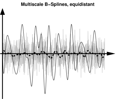
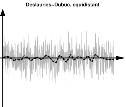
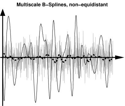
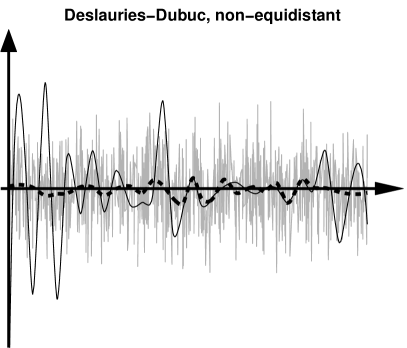
Figure 1: Noise reduction using linear diagonal selection in a multiscale cubic B-spline basis and in a Deslauries-Dubuc scheme with multiscale cubic interpolation: reconstruction with all detail coefficients replaced by zero. Equidistant and non-equidistant observations. In grey line the observations, in black solid line the reconstructions from projections with two primal vanishing moments, in thick black dashed line the reconstructions from the orthogonal projections onto the B-spline or Deslauries-Dubuc bases.

The reconstruction from the Deslauries-Dubuc projection with two vanishing moments shows a large variance on the non-equidistant data, but not on the equidistant equivalent. Reconstruction from a projection with two vanishing moments onto a B-spline basis shows a large variance in both the equidistant and non-equidistant cases. Moreover, further experiments reveal that the variance increases when the B-spline wavelet transform involves more scales. In the Deslauries-Dubuc scheme, there appears to be no such multiscale deterioration. Large variances in that scheme are rather isolated, although possibly devastating, effects from local irregularities in the non-equidistant grid of observations.

Although the large variances are clearly an effect of the non-orthogonality of the transform, the classical numerical condition number sheds no light on the problem. Indeed, on an equispaced, dyadic grid of $n_{J}=2048$ knots, the condition number of the forward Cohen-Daubechies-Feauveau cubic B-spline wavelet with two primal vanishing moments turned out to be $71.9$, and this number is fairly independent from $n_{J}$. On the other hand the condition number of a cubic Deslauries-Dubuc scheme with also two primal vanishing moments is dependent on $n_{J}$ and for $n_{J}=2048$ it equals $203.7$. Nevertheless, the Deslauries-Dubuc scheme on equispaced data shows no problems with large variances. The numerical condition of the wavelet transform is therefore not an adequate description of the non-orthogonality of the transform for statistical applications. The same conclusion holds for the Riesz constants Mallat (2001) in a biorthogonal transformation.

As in B-spline wavelet transforms the increasing variances across scales occur also on equidistant data sets, it is possible to describe them using Fourier transforms. Given a vector after projection $\bm{\varepsilon}_{L}=\mathrm{P}_{L}\bm{\varepsilon}$, define its Fourier transform $Y(\omega)={1\over n}\sum_{\ell=1}^{n}\varepsilon_{L,i}e^{-\ell i\omega}$. By carefully checking the effect of sub- and up-sampling on the Fourier transform, it is fairly straightforward to prove that for $\varepsilon$ uncorrelated and homoscedastic, it holds that

$$E\left|Y(\omega)\right|^{2}={1\over 2^{2(J-L)}}\prod_{j=L}^{J-1}\left|H(2^{j}\omega)\right|\cdot\left(\sum_{k=0}^{2^{J-L}-1}\prod_{j=L}^{J-1}\left|\widetilde{H}(2^{j}(\omega+k\pi/2^{J-L-1}))\right|\right).$$ (69)

In this expression $H(\omega)$ represents the Fourier transform of one row of the one step matrix $H_{j}$. In the equidistant settings, all $H_{j}$ coincide with a single Toeplitz matrix, for which one row suffices to characterise the complete multiscale transform. Obviously, the same definition holds for $\widetilde{H}(\omega)$.

The Fourier analysis cannot be applied to non-equidistant observations, and so it cannot be used to find the best $\widetilde{H}_{j}$ for a given sequence of $H_{j}$. Still under the assumption that the covariance matrix of $\bm{\varepsilon}$ is $\Sigma_{\bm{\varepsilon}}=\sigma^{2}I$, we find that the covariance matrix after projection equals $\Sigma_{\mathrm{P}_{L}\bm{\varepsilon}}=\sigma^{2}\mathrm{P}_{L}\mathrm{P}_{L}^{T}$. Since $\mathrm{P}_{L}\mathrm{P}_{L\perp}=\mathrm{P}_{L\perp}$, and $\mathrm{P}_{L\perp}$ is symmetric and idempotent, it holds that $\mathrm{P}_{L}\mathrm{P}_{L}^{T}-\mathrm{P}_{L\perp}\mathrm{P}_{L\perp}^{T}=\mathrm{P}_{L}(I-\mathrm{P}_{L\perp})\mathrm{P}_{L}^{T}$. The matrix $I-\mathrm{P}_{L\perp}$ is positive semi-definite, so all diagonal elements of $\mathrm{P}_{L}\mathrm{P}_{L}^{T}-\mathrm{P}_{L\perp}\mathrm{P}_{L\perp}^{T}$ must be non-negative, which reads as $\mathrm{var}(\mathrm{P}_{L}\bm{\varepsilon})\geq\mathrm{var}(\mathrm{P}_{L\perp}\bm{\varepsilon})$, this vector inequality holding componentwise. This conclusion is confirmed by the observation in Figure 1. As a result, the variance propagation of a wavelet decomposition applied to uncorrelated homoscedastic observations is described by the nonzero eigenvalues of $\mathrm{P}_{L}\mathrm{P}_{L}^{T}$, i.e., the nonzero singular values of $\mathrm{P}_{L}$. As a summary, define the multiscale variance propagation as follows

Definition 4

(multiscale variance propagation) Given a wavelet transform defined by the sequences of forward and inverse refinement matrices $H_{j}$ and $\widetilde{H}_{j}$, where $j=L,\ldots,J-1$. Let $W_{L}$ and $\widetilde{W}_{L}$ be defined as in (67) and (68), and let $\mathrm{P}_{L}=W_{L}\widetilde{W}_{L}$. Then the multiscale variance propagation equals

$$\kappa_{F}(W_{L},\widetilde{W}_{L})={\|\bm{\sigma}(\mathrm{P}_{L})\|_{2}/\sqrt{n_{L}}}=\|\mathrm{P}_{L}\|_{F}/\sqrt{n_{L}},$$ (70)

where $\bm{\sigma}(\mathrm{P}_{L})$ is the vector of singular values of $\mathrm{P}_{L}$, while $n_{L}$ is the number of columns in $W_{L}$, which is also the number of nonzero singular values of $\mathrm{P}_{L}$. The notation $\|\mathrm{P}_{L}\|_{F}$ stands for the Frobenius norm of $\mathrm{P}_{L}$, whereas $\|\bm{\sigma}(\mathrm{P}_{L})\|_{2}=\sqrt{\bm{\sigma}(\mathrm{P}_{L})^{T}\bm{\sigma}(\mathrm{P}_{L})}$ is the classical Euclidean vector norm.

As an alternative for (70), the multiscale variance propagation can also be defined as

$$\kappa_{2}(W_{L},\widetilde{W}_{L})=\max(\bm{\sigma}(\mathrm{P}_{L}))=\|\mathrm{P}_{L}\|_{2},$$ (71)

where $\|\mathrm{P}_{L}\|_{2}$ denotes the matrix norm induced from the Euclidean vector norm, which is equal to the largest singular value of the matrix.

Using the perfect reconstruction property that $\widetilde{W}_{L}W_{L}=I_{n_{L}}$, it can be proven that all singular values of $\mathrm{P}_{L}=W_{L}\widetilde{W}_{L}$ must be either zero or greater than one. As a consequence, it holds that $\kappa_{F}(W_{L},\widetilde{W}_{L})\geq 1$, and $\kappa_{F}(W_{L},\widetilde{W}_{L})=1$ if and only if $\mathrm{P}_{L}$ is an orthogonal projection.

Given the refinement and detail matrices $\widetilde{H}_{L}^{[0]}$ and $\widetilde{G}_{L}$ that result from the factorisation in Section 2.3, we want to design a sparse update matrix $U_{L}$ that minimises the Frobenius norm of $\mathrm{P}_{L}$, under the constraint that it also preserves a few, say $p$, primal vanishing moments. The index $L$ refers here to the coarsest scale up to the current stage in the design, but $L$ may turn out to be an intermediate scale in the eventual transform.

We first fix which elements of $U_{L}$ will be nonzero. The number of non-zeros must be large enough to cover the $p$ vanishing moments and allow a further optimisation. For a given element $U_{L;r,s}$ this means that we either choose it to be zero, or we optimise its value. We therefore compute the derivative of the Frobenius norm with respect to $U_{L;r,s}$. Since $W_{L}\widetilde{W}_{L}=W_{L}(\widetilde{H}_{L}^{[0]T}+U_{L}\widetilde{G}_{L}^{T})\widetilde{W}_{L+1},$ we find that

$${\partial(W_{L}\widetilde{W}_{L})_{i,j}\over\partial U_{L;r,s}}={\partial(W_{L}U_{L}\widetilde{G}_{L}^{T}\widetilde{W}_{L+1})_{i,j}\over\partial U_{L;r,s}}=W_{L;i,r}(\widetilde{G}_{L}^{T}\widetilde{W}_{L+1})_{s,j}.$$

This we use in

$${\partial\|W_{L}\widetilde{W}_{L}\|_{F}^{2}\over\partial U_{L;r,s}} = {\partial\sum_{i=1}^{n}\sum_{j=1}^{n}(W_{L}\widetilde{W}_{L})_{i,j}^{2}\over\partial U_{L;r,s}}=\sum_{i=1}^{n}\sum_{j=1}^{n}2(W_{L}\widetilde{W}_{L})_{i,j}{\partial(W_{L}\widetilde{W}_{L})_{i,j}\over\partial U_{L;r,s}}$$

$$= 2\sum_{i=1}^{n}\sum_{j=1}^{n}W_{L;i,r}(W_{L}\widetilde{W}_{L})_{i,j}(\widetilde{G}_{L}^{T}\widetilde{W}_{L+1})_{s,j}=\left(W_{L}^{T}W_{L}\widetilde{W}_{L}(\widetilde{G}_{L}^{T}\widetilde{W}_{L+1})^{T}\right)_{r,s}.$$

In this expression, the matrix $\widetilde{W}_{L}=(\widetilde{H}_{L}^{[0]T}+U_{L}\widetilde{G}_{L}^{T})\widetilde{W}_{L+1}$ depends on the update matrix $U_{L}$ that we want to optimise.

Most applications require at least one primal vanishing moment. Therefore, the moment equation (61) is imposed as a constraint in the optimisation process. Using a vector of Lagrange multipliers for each moment, the objective function $K_{L}(U_{L},\bm{\lambda}_{L;m})$ can be written as

$$K_{L}(U_{L},\bm{\lambda}_{L;m})=\|W_{L}\widetilde{W}_{L}\|_{F}^{2}+\sum_{m=0}^{p-1}\bm{\lambda}_{L;m}^{T}(O_{L;m}-U_{L}^{T}M_{L;m}).$$

Given a choice $\mathcal{I}_{L}=\{(r,s)\in\{1,\ldots,n_{L}\}\times\{1,\ldots,n_{L+1}-n_{L}\}|U_{L;r,s}\neq 0$, the $n_{U_{L}}=\#\mathcal{I}_{L}$ equations for the optimisation follow from ${\partial K_{L}\over\partial U_{L;r,s}}=0,$

$$\left(W_{L}^{T}W_{L}U_{L}\widetilde{G}_{L}^{T}\widetilde{W}_{L+1}\widetilde{W}_{L+1}^{T}\widetilde{G}_{L}^{T}\right)_{r,s}=-\left(W_{L}^{T}W_{L}\widetilde{H}_{L}^{[0]T}\widetilde{W}_{L+1}\widetilde{W}_{L+1}^{T}\widetilde{G}_{L}^{T}\right)_{r,s}+\sum_{m=0}^{p-1}\lambda_{L;m;s}M_{L;m;r}.$$ (72)

These equations are completed by $(n_{L+1}-n_{L})p$ moment equations (61).

The set of non-zeros in $U_{L}$ is fixed by the user before the optimisation is carried out. For obvious reasons, its cardinality $n_{U_{L}}$ should be large enough to cope with the moment constraints, i.e., $n_{U_{L}}\geq(n_{L+1}-n_{L})p$. The easiest option is to let $\mathcal{I}_{L}$ be the collection of $\nu$ main and side diagonals. The diagonals have lengths equal to $n_{L+1}-n_{L},n_{L}-1,n_{L+1}-n_{L}-1,n_{L}-2,n_{L+1}-n_{L}-2,\ldots$, summing up to $n_{U_{L}}=\left\lfloor\nu/2\right\rfloor n_{L}+\left\lceil\nu/2\right\rceil(n_{L+1}-n_{L})-\left\lfloor\nu/2\right\rfloor\left\lceil\nu/2\right\rceil$. Since $n_{L+1}-n_{L}$ is the number of odds at scale $j+1$, we have $n_{L+1}-n_{L}\in\{n_{L}-1,n_{L}\}$, and so $n_{U_{L}}=\nu(n_{L+1}-n_{L})-\left\lfloor\nu/2\right\rfloor\left\lceil\nu/2\right\rceil+r_{L}\left\lfloor\nu/2\right\rfloor$, where $r_{L}=2n_{L}-n_{L+1}\in\{0,1\}$. It follows that $n_{U_{L}}\geq(n_{L+1}-n_{L})p$ is not possible for $\nu$ equal to $p$, unless $p=1$. In other words, due to boundary effects, $p$ vanishing moments require more than $p$ diagonals in the final update.

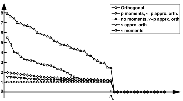
Figure 2: Singular values in descending order for projections $W_{L}\widetilde{W}_{L}$ onto a coarse scale B-spline basis, using several forward transforms $\widetilde{W}_{L}$. In all examples, $\nu=4$ and $p=2$. The orthogonal $\widetilde{W}_{L}$ has no band structure. All other $\widetilde{W}_{L}$ are quadri-diagonal, except for the upper curve, marked with the $\Delta$ signs, which corresponds to a bidiagonal $\widetilde{W}_{L}$.

As an example, depicted in Figure 2, we compute the singular values of the projections $W_{L}\widetilde{W}_{L}$ using cubic B-splines, for the analysis of data that are defined on $n_{J}=1000$ fine scale knots. The fine scale knots were drawn independently from each other from a uniform distribution on $[0,1]$. After $J-L=5$ resolution steps, the coarse scale has a resolution of $n_{L}=32$. Therefore, the matrices $W_{L}$ and $\widetilde{W}_{L}^{T}$ have 1000 rows and 32 columns, from where we know that $\mathrm{rank}(W_{L}\widetilde{W}_{L})=n_{L}=32$. Figure 2 plots the first 53 singular values of the projections in descending order. It is no surprise that the 33rd and beyond are all zero. It is no surprise either that for the orthogonal projection, i.e., for $\widetilde{W}_{L}=(W_{L}^{T}W_{L})^{-1}W_{L}^{T}$, all 32 non-zeros are equal to one. The orthogonal projection matrix $\widetilde{W}_{L}$ is not sparse in the strict sense, although the off-diagonal elements show rapid decay. Therefore, the fully orthogonal projection can be well approximated by a band-limited matrix, using the system of equations in (72). Figure 2 examines the quality of the approximations, showing that a bidiagonal matrix is probably too sparse: even if all free parameters are spent in the optimisation of the singular values, the largest value is close to 8. Three other alternatives for the orthogonal projection use four diagonals. One option is to spend all free parameters on primal vanishing moments. The corresponding wavelets $\psi_{L,k}(x)$ all have four vanishing moments, except those near the boundaries of the interval. The singular values are, however, not controlled, the maximum being close to 6 in this case. The situation may deteriorate quickly in other settings. When all free entries in $U_{L}$ are spent on the minimisation of the singular values, the fourth order approximation is ready for use in statistical applications. But even when two vanishing moments are imposed in combination with a minimisation of the singular values, these values are kept low enough for use in statistical applications. Other experiments, not shown here, confirm that imposing one or two vanishing moments in a scheme that otherwise concentrates on the singular values, is performing nearly as well in terms of singular values, as a scheme that has its entire focus on these singular values.

As a summary for this section, wavelet transforms for use in statistical estimation should be as close as possible to being orthogonal, because reconstructions from non-orthogonal decompositions may suffer from variance blow up. Orthogonality puts, however, serious limitations on the design of a wavelet transform. As an example, orthogonal spline wavelets with compact support do not exist. The numerical notions of condition number and Riesz constants in a biorthogonal transform are not sufficiently adequate for the description of the variance propagation. The design of the wavelet transform proposed in this section therefore focusses directly on the variance and it does so by looking at the combined effect of decomposition and reconstruction.

6 Conclusion and outlook

The first contribution of this paper has been to extend the construction of the Cohen-Daubechies-Feauveau B-spline wavelets towards the case of non-equidistant knots. The new construction is based on the factorisation of two-scale or refinement equations into lifting steps. An interesting topic for further research is to investigate the same methodology for other spline wavelets.

The second contribution has been the design of a numerical method to find fine scaling coefficients from function values, in a way that performs well when the function is observed with noise. Future research could improve the method by making it adaptive to jumps or other singularities. In the neighbourhood of jumps, the benefit from a perfect reconstruction of power functions is limited, so a local relaxation of these conditions may yield sharper reconstructions.

Finally, the third contribution has been a modification of the Cohen-Daubechies-Feauveau wavelet transform for specific use in statistical applications, making sure to control the propagation of the variance on the wavelet coefficients at successive scales. The focus on the variance propagation in the design of the transform allows us to relax the stringent orthogonality condition and to construct a basis of compactly supported spline wavelets in which non-linear processing leads to a reconstruction with a well controlled bias-variance balance.

Acknowledgement

Research support by the IAP research network grant nr. P7/06 of the Belgian government (Belgian Science Policy) is gratefully acknowledged.

Appendices

Appendix A Available software - reproducible research

All transforms presented in this article have been implemented in the latest version of ThreshLab, a Matlab®software package available for download from
http://homepages.ulb.ac.be/~majansen/software/threshlab.html.

The forward and inverse B-spline wavelet transforms are carried out by the routines FWT_2Gspline.m and IWT_2Gspline.m. Several alternatives for the retrieval of appropriate fine scaling coefficients from noisy observations, explained in Section 4, are implemented in finescaleBsplinecoefs.m. The use of this routine is illustrated in illustratefinescalecoefs.m.

In particular, the experiment in Figure 1 is set up in the routine illustratevarianceprojection.m. The singular value plots in Figure 2 have been generated using illustrate_updateLSapprxprimmom.m.

Appendix B Proofs for Theorems 5,3, and 4

The proofs are given for the sake of self-containment. The results are well-known in literature.

B.1 Proof of Theorem 5

The summation in (5) contains $n_{j}-\left\lceil\widetilde{p}/2\right\rceil-\left\lfloor\widetilde{p}/2\right\rfloor=n_{j}-\widetilde{p}$ B-spline functions. All B-splines have mutually unequal supports, and are thus linearly independent. On the other hand, $I_{j}$ consists of $n_{j}-2\widetilde{p}+1$ subintervals $[x_{j,k},x_{j,k+1})$, with $\widetilde{p}$ degrees of freedom on each of them. The continuous derivatives in each interior knot consume $(n_{j}-2\widetilde{p})\times(\widetilde{p}-1)$ of these degrees of freedom, leaving us with a vector space of dimension $n_{j}-\widetilde{p}$. $\Box$

B.2 Proof of Theorem 3

1. Expression (11) follows from (8), applied for $f_{j}(x)=x^{q}$. The left hand side of (8) can then be written as

   $$qx^{q-1}=q\sum_{k\in\mathbbm{Z}}\widetilde{x}_{j,k-\widetilde{r}^{\prime}}^{\left[\widetilde{p}-1,q-1\right]}\varphi_{j,k-\widetilde{r}^{\prime}}^{\left[\widetilde{p}-1\right]}(x),$$

   whereas the right hand side becomes

   $$qx^{q-1}=(\widetilde{p}-1)\sum_{k\in\mathbbm{Z}}{\widetilde{x}_{j,k}^{\left[\widetilde{p},q\right]}-\widetilde{x}_{j,k-1}^{\left[\widetilde{p},q\right]}\over x_{j,k+\left\lceil\widetilde{p}/2\right\rceil-1}-x_{j,k-\left\lfloor\widetilde{p}/2\right\rfloor}}\varphi_{j,k-\widetilde{r}^{\prime}}^{\left[\widetilde{p}-1\right]}(x).$$

   Identification of the terms in the decomposition leads to (11).

2. Next, it can be verified that all solutions for $\widetilde{x}_{j,k}^{\left[\widetilde{p},1\right]}$ in (11) must satisfy

   $$\widetilde{x}_{j,k}^{\left[\widetilde{p},1\right]}={1\over\widetilde{p}-1}\sum_{i=1-\left\lfloor\widetilde{p}/2\right\rfloor}^{\left\lceil\widetilde{p}/2\right\rceil-1}x_{j,k+i}-{1\over\widetilde{p}-1}\sum_{i=1-\left\lfloor\widetilde{p}/2\right\rfloor}^{\left\lceil\widetilde{p}/2\right\rceil-1}x_{j,i}+s_{j,0}^{\left[\widetilde{p},1\right]}.$$

   On the other hand, $\widetilde{x}_{j,k}^{\left[\widetilde{p},1\right]}$ must be independent from the $\widetilde{p}-1$ knots $x_{j,i}$ around $x_{j,0}$ if $k>\widetilde{p}$. So take $x_{j,i}$ symmetric around $x_{j,0}=0$. Then, obviously,

   $${1\over\widetilde{p}-1}\sum_{i=1-\left\lfloor\widetilde{p}/2\right\rfloor}^{\left\lceil\widetilde{p}/2\right\rceil-1}x_{j,i}=0.$$

   On the other hand, $s_{j,0}^{\left[\widetilde{p},1\right]}=0$, as the corresponding basis function is even. This leads to (12).

3. The proof for (13) is similar to that for (12), following an induction argument on $\widetilde{p}$.

$\Box$

B.3 Proof of Theorem 4

Consider $x\in(x_{j,k},x_{j,k+1})\subset I_{j}$, then $x\in S_{j,m}\Leftrightarrow l_{m}<k+1\mbox{ and }r_{m}>k\Leftrightarrow k-\left\lceil\widetilde{p}/2\right\rceil+1\leq m\leq k+\left\lfloor\widetilde{p}/2\right\rfloor.$ Then in $x$, it holds that

$$\left[1\,\,x\,\,x^{2}\,\,\ldots x^{\widetilde{p}-1}\right]=\left[\varphi_{j,k-\left\lceil\widetilde{p}/2\right\rceil+1}^{\left[\widetilde{p}\right]}(x)\,\,\ldots\,\,\varphi_{j,k+\left\lfloor\widetilde{p}/2\right\rfloor}^{\left[\widetilde{p}\right]}(x)\right]\,\widetilde{X},$$

where $\widetilde{X}_{m-k+\left\lceil\widetilde{p}/2\right\rceil,q+1}=\widetilde{x}_{j,m}^{\left[\widetilde{p},q\right]}.$ It can be verified that $\widetilde{X}$ is non-singular, so we find an expression for the basis functions on the subinterval $(x_{j,k},x_{j,k+1})$,

$$\left[\varphi_{j,k-\left\lceil\widetilde{p}/2\right\rceil+1}^{\left[\widetilde{p}\right]}(x)\,\,\ldots\,\,\varphi_{j,k+\left\lfloor\widetilde{p}/2\right\rfloor}^{\left[\widetilde{p}\right]}(x)\right]=\left[1\,\,x\,\,x^{2}\,\,\ldots x^{\widetilde{p}-1}\right]\,\widetilde{X}^{-1},$$ (73)

all other basis functions being zero on this subinterval. It follows that on each subinterval, the basis functions must be polynomials, and the polynomials are uniquely defined by (73). As from Theorem 3, we know that the power functions have the coefficients $\widetilde{x}_{j,m}^{\left[\widetilde{p},q\right]}$ in a B-spline basis, the polynomials defined by (73) must coincide with the B-splines on that interval. $\Box$

Appendix C Constructive proof for the factorisation in Theorem 24

The factorisation is based on the approach in Daubechies and Sweldens (1998). Because of the non-equidistant knots, it proceeds column by column in the refinement matrix. The proof also makes use of the band structure of a matrix. For the sake of simplicity, and without any impact on the applicability of the argument, we ignore occasional zeros within the nonzero band of $H_{j,e}^{[s]}$ or $H_{j,o}^{[s]}$. In each column of these matrices, we take the same number of rows into consideration, equal to the bandwidth of the whole matrix, even if that particular row has actually less non-zeros.

Consider first the case where $H_{j,e}^{[s]}$ has a larger bandwidth than $H_{j,o}^{[s]}$. This is only possible if the first and last nonzero in each column of $H_{j}$ is situated on an even row. Denote by $2k_{1}(\ell)$ the first nonzero row in column $\ell$ of $H_{j}$ and by $2k_{2}(\ell)$ the last nonzero row in the same column. Then the $\ell$th column of (23) reads as

$$H_{j,2k,\ell}^{[s]}=H_{j,2k,\ell}^{[s+1]}-\sum_{m=k_{1}(\ell)}^{k_{2}(\ell)}U_{j,k,m}^{[s+1]}H_{j,2m+1,\ell}^{[s]},$$ (74)

We assume that $k_{1}(\ell)$ and $k_{2}(\ell)$ are strictly increasing functions, otherwise a more careful design of the update step is needed. Let $\ell_{2}(k)$ be the inverse of $k_{1}(\ell)$, i.e., $\ell_{2}(k_{1}(\ell))=\ell$. In words, $\ell_{2}(k)$ is the last column on row $k$ with a nonzero element. In a similar way, let $\ell_{1}(k)$ be the inverse of $k_{2}(\ell)$. In a given column $\ell$, we impose for $k=k_{1}(\ell)$ and for $k=k_{2}(\ell)$ that $H_{j,2k,\ell}^{[s+1]}=0$, so that the number of non-zeros in column $\ell$ of $H_{j,e}^{[s+1]}$ equals $k_{2}(\ell)-k_{1}(\ell)-1$. Note that the number of nonzero rows equals $k_{2}(\ell)-k_{1}(\ell)+1$ for $H_{j,e}^{[s]}$ and $k_{2}(\ell)-k_{1}(\ell)$ for $H_{j,o}^{[s]}$. For $k=k_{1}(\ell)$, and for $k=k_{2}(\ell)$, we obtain the two equations of the form

$$H_{j,2k,\ell}^{[s]}=-\sum_{m=k_{1}(\ell)}^{k_{2}(\ell)-1}U_{j,k,m}^{[s+1]}H_{j,2m+1,\ell}^{[s]}.$$ (75)

These two equations contain as unknowns two partial rows in matrix $U_{j}^{[s+1]}$. Instead of solving the two equations for fixed $\ell$, we consider the two equations for given $k$, by looking at $\ell=\ell_{2}(k)$ and $\ell=\ell_{1}(k)$.

For $k=k_{1}(\ell)$, i.e., $\ell=\ell_{2}(k)$, we set $U_{j,k,m}^{[s+1]}=0$ for all $m=k+1,\ldots,k_{2}(\ell_{2}(k))-1$, while for $m=k$, we must then take

$$U_{j,k,k}^{[s+1]}=-H_{j,2k,\ell_{2}(k)}^{[s]}/H_{j,2k+1,\ell_{2}(k)}^{[s]},$$ (76)

in order to satisfy (75) for $k=k_{1}(\ell)$ or $\ell=\ell_{2}(k)$.

For $k=k_{2}(\ell)$, i.e., $\ell=\ell_{1}(k)$, we set $U_{j,k,m}^{[s+1]}=0$ for all $m=k_{1}(\ell_{1}(k)),\ldots,k-2$, while for $m=k-1$, we must then take

$$U_{j,k,k-1}^{[s+1]}=-H_{j,2k,\ell_{1}(k)}^{[s]}/H_{j,2k-1,\ell_{1}(k)}^{[s]},$$ (77)

in order to satisfy (75) for $k=k_{2}(\ell)$ or $\ell=\ell_{1}(k)$.

Once the diagonal and the lower diagonal of $U_{j}^{[s+1]}$ has been found, all the other entries of this matrix can be filled with zeros. This leaves us with $k_{2}(\ell)-k_{1}(\ell)-1$ equations of the form (74). Each of these equations allows us to find exactly one element in column $\ell$ of $H_{j,e}^{[s+1]}$.

The case where the bandwidth of $H_{j,o}^{[s]}$ is larger than that of $H_{j,e}^{[s]}$ is treated in a similar way. The case where the bandwidths of $H_{j,e}^{[s]}$ and $H_{j,o}^{[s]}$ are equal can be reduced to the first case if we artificially increase the bandwidth of $H_{j,e}^{[s]}$, by taking an additional zero into account in each column of $H_{j,e}^{[s]}$. $\Box$

Appendix D Proof of Proposition 1

First, it can be checked that (26) holds for any $\widetilde{p}$ and for $q=1$ and for $q=\widetilde{p}-1$. More precisely, a bit of calculations show that from (12), it follows indeed that,

$$\widetilde{t}_{j,k}^{\left[\widetilde{p},1,L1\right]}={t_{j,k+\widetilde{p}-1}-t_{j,k+1}\over t_{j,k+\widetilde{p}}-t_{j,k}}\,\left(t_{j,k}+\sum_{i=2}^{\widetilde{p}-2}t_{j,k+i}+t_{j,k+\widetilde{p}}\right).$$ (78)

In a similar way, starting from (13), we arrive at

$$\widetilde{t}_{j,k}^{\left[\widetilde{p},\widetilde{p}-1,L1\right]}={t_{j,k+\widetilde{p}-1}-t_{j,k+1}\over t_{j,k+\widetilde{p}}-t_{j,k}}\,\left(t_{j,k}\cdot\prod_{i=2}^{\widetilde{p}-2}t_{j,k+i}\cdot t_{j,k+\widetilde{p}}\right).$$ (79)

As a result, for $\widetilde{p}=1,2$ the result holds for all $q=0,\ldots,\widetilde{p}-1$. This is the basis for the subsequent induction argument.

Using the recursion in (14), we can find the coefficient $\widetilde{t}_{j,k}^{\left[\widetilde{p},q,L1b\right]}$ in two steps. First we define $\widetilde{t}_{j,k}^{\left[\widetilde{p},q,L1a\right]}$ as the coefficient that results from taking out $t_{j,k+1}$ from $\widetilde{t}_{j,k}^{\left[\widetilde{p},q\right]}$ and replacing it by $t_{j,k}$. This intermediate coefficient equals

$$\widetilde{t}_{j,k}^{\left[\widetilde{p},q,L1a\right]}=\widetilde{t}_{j,k}^{\left[\widetilde{p},q\right]}+{q\over\widetilde{p}-1}\,\widetilde{t}_{j,k+1}^{\left[\widetilde{p}-1,q-1\right]}\,\left(t_{j,k}-t_{j,k+1}\right).$$

We define a similar coefficient for $\widetilde{p}-1$ and $q-1$.

$$\widetilde{t}_{j,k}^{\left[\widetilde{p}-1,q-1,L1a\right]}=\widetilde{t}_{j,k}^{\left[\widetilde{p}-1,q-1\right]}+{q-1\over\widetilde{p}-2}\,\widetilde{t}_{j,k+1}^{\left[\widetilde{p}-2,q-2\right]}\,\left(t_{j,k}-t_{j,k+1}\right).$$

Next, we take out $t_{j,k+\widetilde{p}-1}$ from $\widetilde{t}_{j,k}^{\left[\widetilde{p},q,L1a\right]}$ and replace it with $t_{j,k+\widetilde{p}}$. In order to apply (14), we need the power coefficient of degree $\widetilde{p}-1$ for $q-1$ based on all remaining knots in $\widetilde{t}_{j,k}^{\left[\widetilde{p},q,L1a\right]}$. This is exactly $\widetilde{t}_{j,k}^{\left[\widetilde{p}-1,q-1,L1a\right]}$. We thus find

$$\widetilde{t}_{j,k}^{\left[\widetilde{p},q,L1b\right]}=\widetilde{t}_{j,k}^{\left[\widetilde{p},q,L1a\right]}+{q\over\widetilde{p}-1}\,\widetilde{t}_{j,k}^{\left[\widetilde{p}-1,q-1,L1a\right]}\left(t_{j,k+\widetilde{p}}-t_{j,k+\widetilde{p}-1}\right).$$

Using the expressions above for $\widetilde{t}_{j,k}^{\left[\widetilde{p},q,L1a\right]}$ and for $\widetilde{t}_{j,k}^{\left[\widetilde{p}-1,q-1,L1a\right]}$, this can further be developed into

$$\begin{array}[]{rl}\displaystyle\widetilde{t}_{j,k}^{\left[\widetilde{p},q,L1b\right]}=\widetilde{t}_{j,k}^{\left[\widetilde{p},q\right]}+{q\over\widetilde{p}-1}&\!\!\!\!\left[\widetilde{t}_{j,k}^{\left[\widetilde{p}-1,q-1\right]}(t_{j,k}+t_{j,k+\widetilde{p}}-t_{j,k+1}-t_{j,k+\widetilde{p}-1})\right.\\ &\displaystyle\left.+{q-1\over\widetilde{p}-2}\,\widetilde{t}_{j,k+1}^{\left[\widetilde{p}-2,q-2\right]}(t_{j,k}-t_{j,k+1})(t_{j,k+\widetilde{p}}-t_{j,k+1})\right].\end{array}$$ (80)

Expression (80) can be substituted in the right hand side of (26). We now work on $\widetilde{t}_{j,k}^{\left[\widetilde{p},q,L1\right]}$ in the left hand side, starting from its definition in (1), and using once more the recursion (14). We find

$$\widetilde{t}_{j,k}^{\left[\widetilde{p},q,L1\right]} = {t_{j,k+\widetilde{p}-1}-t_{j,k+1}\over t_{j,k+\widetilde{p}}-t_{j,k}}\,\,\widetilde{t}_{j,k}^{\left[\widetilde{p},q\right]}-{q\over\widetilde{p}-1}\,\,{1\over t_{j,k+\widetilde{p}}-t_{j,k}}\cdot$$

$$\left[\widetilde{t}_{j,k+1}^{\left[\widetilde{p}-1,q-1\right]}(t_{j,k+\widetilde{p}}-t_{j,k+1})(t_{j,k+1}-t_{j,k})+\widetilde{t}_{j,k}^{\left[\widetilde{p}-1,q-1\right]}(t_{j,k}-t_{j,k+\widetilde{p}-1})(t_{j,k+\widetilde{p}}-t_{j,k+\widetilde{p}-1})\right].$$

For the last factor in this expression, we use again the recursion (14), this time for

$$\widetilde{t}_{j,k+1}^{\left[\widetilde{p}-1,q-1\right]}=\widetilde{t}_{j,k}^{\left[\widetilde{p}-1,q-1\right]}+{q-1\over\widetilde{p}-2}\,\widetilde{t}_{j,k+1}^{\left[\widetilde{p}-2,q-2\right]}\,\left(t_{j,k+\widetilde{p}-1}-t_{j,k+1}\right).$$

Substitution of this recursion, followed by straightforward algebraic manipulation, amounts to (26), thereby completing the proof.

Correspondence address

Maarten Jansen
Departments of Mathematics and Computer Science,
Université Libre de Bruxelles
Boulevard du Triomphe
Campus Plaine, CP213
B-1050 Brussels - Belgium
maarten.jansen@ulb.ac.be

References

- Battle (1987) G. Battle. A block spin construction of ondelettes. Part I: Lemarié functions. Comm. Math. Phys., 110(4):601–615, 1987.
- Bertram (2004) M. Bertram. Lifting biorthogonal B-spline wavelets. In G. Brunnett, B. Hamann, H. Müller, and L. Linsen, editors, Geometric Modeling for Scientific Visualization, number IX in Mathematics and Visualization, pages 153–159. Springer-Verlag, 2004.
- Chern (1999) I-L. Chern. Interpolating wavelets and difference wavelets. In Proceedings of the Centre for Mathematics and its Applications, volume 37, pages 133–147, 1999.
- Chui and Wang (1992) C.K. Chui and J.Z. Wang. On compactly supported spline wavelets and a duality principle. Trans. Amer. Math. Soc., 330(2):903–915, 1992.
- Cohen et al. (1992) A. Cohen, I. Daubechies, and J. Feauveau. Bi-orthogonal bases of compactly supported wavelets. Comm. Pure Appl. Math., 45:485–560, 1992.
- Daubechies (1993) I. Daubechies. Orthonormal bases of compactly supported wavelets II: Variations on a theme. SIAM J. Math. Anal., 24(2):499–519, 1993.
- Daubechies and Sweldens (1998) I. Daubechies and W. Sweldens. Factoring wavelet transforms into lifting steps. J. Fourier Anal. Appl., 4(3):245–267, 1998.
- Daubechies et al. (1999a) I. Daubechies, I. Guskov, P. Schröder, and W. Sweldens. Wavelets on irregular point sets. Phil. Trans. R. Soc. Lond. A, 357:2397–2413, 1999a.
- Daubechies et al. (1999b) I. Daubechies, I. Guskov, and W. Sweldens. Regularity of irregular subdivision. Constructive Approximation, 15(3):381–426, 1999b.
- Daubechies et al. (2001) I. Daubechies, I. Guskov, and W. Sweldens. Commutation for irregular subdivision. Constructive Approximation, 17(4):479–514, 2001.
- Daubechies et al. (2004) I. Daubechies, M. Defrise, and C. De Mol. An iterative thresholding algorithm for linear inverse problems with a sparsity constraint. Comm. Pure Appl. Math., 57:1413–1457, 2004.
- de Boor (2001) C. de Boor. A Practical Guide to Splines. Springer, New York, 2001. Revised Edition.
- Deslauriers and Dubuc (1987) G. Deslauriers and S. Dubuc. Interpolation dyadique. In Fractales, Dimensions Non-entières et Applications, pages 44–55. Masson, Paris, 1987.
- Deslauriers and Dubuc (1989) G. Deslauriers and S. Dubuc. Symmetric iterative interpolation processes. Constructive Approximation, 5:49–68, 1989.
- Donoho and Yu (1999) D. L. Donoho and T.P.Y. Yu. Deslauries-Dubuc: ten years after. In S. Dubuc and G. Deslauriers, editors, Spline Functions and the Theory of Wavelets, CRM Proceedings and Lecture Notes. American Mathematical Society, 1999.
- Dubeau and J. Savoie (1995) F. Dubeau and J. J. Savoie. Explicit error bounds for spline interpolation on a uniform partition. J. Approx. Theory, 82:1–14, 1995.
- Eubank (1999) R. L. Eubank. Nonparametric regression and spline smoothing, volume 157 of Statistics: Textbooks and Monographs. Marcel Dekker Inc., New York, 2 edition, 1999. ISBN 0-8247-9337-4.
- Fahmy (2008) G. Fahmy. Bspline based wavelets with lifting implementation. In Proceedings of the IEEE International Symposium on Signal Processing and Information Technology, ISSPIT 2008, volume 37, pages 85–89, 2008.
- Girardi and Sweldens (1997) M. Girardi and W. Sweldens. A new class of unbalanced Haar wavelets that form an unconditional basis for on general measure spaces. J. Fourier Anal. Appl., 3(4):457–474, 1997.
- Green and Silverman (1994) P. J. Green and B. W. Silverman. Nonparametric regression and generalized linear models: A roughness penalty approach, volume 58 of Monographs on Statistics and Applied Probability. Chapman & Hall, London, 1994. ISBN 0-412-30040-0.
- Jansen and Oonincx (2005) M. Jansen and P. Oonincx. Second generation wavelets and applications. Springer, 2005.
- Jansen et al. (2009) M. Jansen, G. Nason, and B. Silverman. Multiscale methods for data on graphs and irregular multidimensional situations. Journal of the Royal Statistical Society, Series B, 71(1):97–125, 2009.
- Landweber (1951) L. Landweber. An iterative formula for fredholm integral equations of the first kind. Amer. J. Math., 73:615–624, 1951.
- Lee (1996) E.T.Y. Lee. Marsden’s identity. Comp. Aided Geom. Design, 13(4):287–305, June 1996.
- Lemarié (1988) P.-G. Lemarié. Ondelettes à localisation exponentielles. J. Math. Pures et Appl., 67(3):227–236, 1988.
- Li et al. (2005) D. Li, K. Qin, and H. Sun. Curve modeling with constrained B-spline wavelets. Computer Aided Geometric Design, 22:45–56, 2005.
- Lyche et al. (2001) T. Lyche, K. K. Msorken, and E. Quak. Theory and algorithms for nonuniform spline wavelets. In N. Dyn, D. Leviatan, D. Levin, and A. Pinkus, editors, Multivariate Approximation and Applications, pages 152–187. Cambridge University Press, 2001.
- Mallat (2001) S. Mallat. A Wavelet Tour of Signal Processing. Academic Press, 2 edition, 2001.
- Pan and Yao (2009) R. Pan and Z. Yao. Biorthogonal nonuniform B-spline wavelets based on a discrete norm. Computer Aided Geometric Design, 26:480–492, 2009.
- Prestin and Quak (2005) J. Prestin and E. Quak. Periodic and Spline Multiresolution Analysis and the Lifting Scheme. In N. A. Dodgson, M. S. Floater, and M. A. Sabin, editors, Advances in Multiresolution for Geometric Modelling, number X in Mathematics and Visualization, pages 369–390. Springer-Verlag, 2005.
- Qu and Gregory (1992) R. Qu and J. Gregory. A subdivision algorithm for non-uniform B-splines. In S.P. Singh, editor, Approximation Theory, Wavelets and Applications, volume 356 of NATO ASI Series C, pages 423–436, 1992.
- Ruppert et al. (2003) D. Ruppert, M.P. Wand, and R. Carroll. Semiparametric Regression. Cambridge University Press, Cambridge, UK, 2003.
- Strang and Nguyen (1996) G. Strang and T. Nguyen. Wavelets and Filter Banks. Wellesley-Cambridge Press, Box 812060, Wellesley MA 02181, fax 617-253-4358, 1996.
- Sweldens (1996) W. Sweldens. The lifting scheme: A custom-design construction of biorthogonal wavelets. Appl. Comp. Harmon. Anal., 3(2):186–200, 1996.
- Sweldens (1998) W. Sweldens. The lifting scheme: a construction of second generation wavelets. SIAM J. Math. Anal., 29(2):511–546, 1998.
- Sweldens and Piessens (1994) W. Sweldens and R. Piessens. Quadrature formulae and asymptotic error expansions for wavelet approximations of smooth functions. SIAM J. Numer. Anal., 31(4):1240–1264, 1994.
- Sweldens and Schröder (1996) W. Sweldens and P. Schröder. Building your own wavelets at home. In Wavelets in Computer Graphics, ACM SIGGRAPH Course Notes, pages 15–87. ACM, 1996.
- Unser et al. (1992) M. Unser, A. Aldroubi, and M. Eden. On the asymptotic convergence of B-spline wavelets to gabor functions. IEEE Trans. Information Theory, 38(2):864–872, 1992.
- Unser et al. (1993) M. Unser, A. Aldroubi, and M. Eden. A family of polynomial spline wavelet transforms. Signal Processing, 30(2):141–162, 1993.
- Unser (1997) M. A. Unser. Ten good reasons for using Spline Wavelets. In A. Aldroubi, A. F. Laine, and M. A. Unser, editors, Wavelet Applications in Signal and Image Processing V, volume 3169, pages 422–431, 10 1997.
- Van Aerschot et al. (2006) W. Van Aerschot, M. Jansen, and A. Bultheel. Adaptive splitting for stabilizing 1-d wavelet decompositions. Signal Processing, 86(9):2447–2463, 2006.
- Vanraes et al. (2002) E. Vanraes, M. Jansen, and A. Bultheel. Stabilizing wavelet transforms for non-equispaced data smoothing. Signal Processing, 82(12):1979–1990, December 2002.
- Vanraes et al. (2004) E. Vanraes, J. Maes, and A. Bultheel. Powell-Sabin spline wavelets. International Journal of Wavelets, Multiresolution and Information Processing, 2(1):23–42, 2004.
- Xiang et al. (2007) J. W. Xiang, X. F. Chen, Z. J. He, and H. B. Dong. The construction of 1d wavelet finite elements for structural analysis. Comput. Mech., 40:325–339, 2007.