Automated NLO/NLL Monte Carlo programs for the LHC

Abstract

The interpretation of experimental measurements at the LHC requires accurate theoretical predictions for exclusive observables, and in particular the summation of soft and collinear radiation to all orders in perturbation theory. We report on recent progress towards the automated calculation of multi-parton LHC cross sections at next-to-leading order in QCD, including the summation of next-to-leading logarithmic corrections through the combination with parton showers.

1 Introduction

Theoretical calculations within fixed-order perturbation theory allow for accurate predictions of inclusive observables like total cross sections. The analysis and interpretation of experimental signatures at the LHC, however, require theoretical predictions for exclusive final states, i.e. predictions for differential distributions or cross sections with cuts on kinematic variables. Higher-order calculations for such exclusive final states involve in general large corrections from soft or collinear parton emission, which need to be summed to all orders. An efficient way to achieve such a summation is through a parton shower. Parton showers typically include the leading logarithmic contributions from soft and collinear gluon or quark emission to all orders in perturbation theory. They form a central part of Monte Carlo event generators and are thus essential to connect theoretical models with realistic experimental signatures. On the other hand, standard parton shower event generators often rely on leading-order expressions for the hard scattering processes and can therefore not predict inclusive cross sections accurately.

A central goal of recent and current theoretical work in LHC phenomenology is thus the automated calculation of next-to-leading (NLO) LHC cross sections including the summation of large corrections from multiple quark and gluon emission through parton showers. Such a calculation should combine the accuracy of NLO predictions for inclusive cross sections with the power of parton shower Monte Carlo programs to reliably describe differential distributions and cross sections with cuts on kinematic variables. A naive combination of NLO calculations with parton showers would, however, lead to double counting of higher-order contributions that are included in both the NLO cross section and the parton shower. These contributions have to be identified and subtracted from the calculation by means of a matching procedure.

Much work in recent years has been devoted to the formulation of matching schemes that allow for a consistent combination of parton showers and NLO calculations including loop-corrections [1, 2, 3, 4, 5, 6, 7, 8, 9, 10, 11, 12, 13, 14, 15, 16]. So far, however, only few publicly available computer codes exist that implement such schemes, including in particular Mc@NLO [17], Powheg [18], Sherpa [19] and Madgraph5_aMc@NLO [20]. The problem of double counting contributions that are included in both the NLO calculation and the parton shower has been solved in all approaches in a similar way: The parton shower evolution is generically described by a Sudakov factor of the form

$$\exp\left(-\int_{Q^{2}}^{\infty}\frac{d\bar{q}^{2}}{\bar{q}^{2}}\int_{0}^{1}dz\ \frac{\alpha_{s}}{2\pi}\,P_{g/q}(\bar{q}^{2},z)\right)\,,$$

shown here for gluon emission off a quark with virtuality $Q^{2}$. In the collinear limit $\bar{q}^{2}\to 0$ the function $P_{g/q}(\bar{q}^{2},z)$ reduces to the Altarelli-Parisi splitting function. The Sudakov factor includes short-distance contributions which are also part of the NLO cross section and which can be identified by expanding the exponential in powers of $\alpha_{s}$. When combining parton showers with NLO calculations these contributions need to be subtracted to avoid double counting.

Early work by many authors has focused on implementing specific processes into the Mc@NLO program and within the Powheg framework. While the original Mc@NLO code is very successful and now includes a large number of processes, it is tied strongly to the parton shower of Herwig (both Herwig6 and Herwig++). This restriction has been lifted recently within Madgraph5_aMc@NLO, which is not only fully automatic, but also parton shower independent and may be used with various versions of Herwig and Pythia. We note that Sherpa contains an implementation of Mc@NLO as well. Powheg, on the other hand, allowed for matching with a generic parton shower from the beginning and could thus be interfaced with various Monte Carlo programs. In practice, the implementation of specific processes has been greatly simplified thanks to the Powheg-Box tool. In each of the frameworks, multiple parton emission is summed at the leading-logarithmic (LL) level only (although leading-color subleading logarithmic effects might be included in parton showers based on NLO subtraction schemes, such as the Catani-Seymour subtraction), and the results can thus not compete with the accuracy of dedicated resummation calculations which are routinely performed at next-to-leading logarithmic accuracy (NLL).

The formulation and improvement of parton showers, which are in general based on various assumptions and approximations, has also been addressed by various authors recently [21, 22, 23, 24, 25, 26, 27, 28, 29, 30, 31, 32, 33, 34, 35, 36, 37]. Notably, Refs. [23, 26, 27, 32] have proposed a parton shower that includes quantum interference, spin correlations and sub-leading color effects. Interference is treated in standard parton showers only approximately by means of angular ordering, while spin information is generally ignored completely. Spin correlations, on the other hand, are crucial for example to explore new physics models in cascade decays at the LHC. While Refs. [23, 26, 27, 32] describe the theoretical formulation of parton showers with quantum interference, the first implementation [35] so far is based on the standard spin-averaged and leading-color treatment of parton splitting only.

The set-up of the parton shower also has implications for the matching with NLO calculations. If the splitting functions of the parton shower, $P_{ij}(\bar{q}^{2},z)$, and the momentum mapping follow closely the definition of the subtraction terms used to regularize the soft and collinear divergences in the NLO calculation, then the matching is simplified considerably. With that in mind, various authors have formulated parton showers that are based on commonly used subtraction schemes [25, 24].

To improve on existing NLO plus parton shower implementations, quantum interference contributions, spin correlations and sub-leading color effects in the parton shower should be included systematically. Ultimately, one would like to develop a fast and numerically robust code for the automated calculation of multi-parton LHC cross sections at next-to-leading order, including the summation of next-to-leading logarithmic corrections through combination with parton showers. In this contribution we shall describe recent progress towards this goal.

The article is structured as follows. In Section 2 we shall describe the construction of a NLO subtraction scheme as derived from a NLL parton shower, and its implementation into the program package Helac-NLO. Section 3 reports on the application of such a scheme for the automated calculation of NLO-QCD corrections to the production of four bottom quarks at the LHC. Section 4 finally discusses progress towards developing and implementing a NLL parton shower and the matching with Helac-NLO. We conclude in Section 5.

2 Subtraction schemes for NLO-QCD calculations

In the following, a new subtraction scheme based on a parton shower introduced by Nagy and Soper [23] is described. This new subtraction has been implemented in the publicly available Helac-Dipoles software [38] and has already been tested in the calculation of the NLO QCD corrections to $pp\to b\bar{b}b\bar{b}+X$ production at the LHC (see the next section for more details). Our main motivation, however, was to provide a framework for a simple matching between a fixed-order calculation and the new parton shower. However, before addressing this issue, the problem of the integration of subtraction terms over the unresolved phase space needed to be solved. This is the non-trivial part of any subtraction scheme. Contrary to the usual practice at NLO, we did not perform involved analytic integrations, but rather used a semi-numerical approach. After a suitable parameterization, numerical integrations, inspired by recent NNLO methods [39], have been performed. This has allowed us to cover both massless and massive cases with comparable effort. Let us emphasize that our semi-numerical approach distinguishes our work from earlier publications on the subject presented e.g.  in Refs. [40, 41, 42].

Let us start with the inclusive NLO QCD cross section for a generic process involving $m+1$ final-state QCD partons with momenta $p_{a}+p_{b}\to p_{1}+\cdots+p_{m+1}$, which can be written as follows

$$\sigma_{\rm NLO} = \int_{m}d\Phi_{m}\,\,\mathcal{A}^{B}(\{p\}_{m})\,\,F_{m}$$

$$+ \int_{m+1}d\Phi_{m+1}\,\,\mathcal{A}^{R}(\{p\}_{m+1})\,\,F_{m+1}$$

$$+ \int_{m}d\Phi_{m}\,\,\mathcal{A}^{V}(\{p\}_{m})\,\,F_{m}$$

$$+ \int_{0}^{1}dx\int_{m}d\Phi_{m}(x)\,\,\mathcal{A}^{C}(x,\{p\}_{m})\,\,F_{m}$$

where

$$\mathcal{A}^{B}\equiv|\mathcal{M}^{\mbox{\scriptsize{Born}}}|^{2}\,,~{}~{}~{}~{}~{}~{}~{}\mathcal{A}^{R}\equiv|\mathcal{M}^{\mbox{\scriptsize{Real}}}|^{2}\,,\;\;\;\>\>$$

$$\mathcal{A}^{V}\equiv 2\,\Re\left[\mathcal{M}^{\mbox{\scriptsize{Born}}}\,(\mathcal{M}^{\mbox{\scriptsize{1-Loop}}})^{*}\right]\,,$$

and $\mathcal{M}^{\mbox{\scriptsize{Born}}}$, $\mathcal{M}^{\mbox{\scriptsize{1-Loop}}}$, $\mathcal{M}^{\mbox{\scriptsize{Real}}}$ describe the Born, one-loop and real-emission matrix elements, respectively. The integration measure for the $m-$ and the $m+1-$parton phase space is denoted by $d\Phi_{m}$ and $d\Phi_{m+1}$, whereas $F_{m}$ and $F_{m+1}$ are the jet functions.

For $m$ well separated hard jets, the Born contribution is finite, whereas the virtual and the real-emission terms are individually divergent due to the presence of soft and collinear singularities. For an infrared-safe definition of partonic jets, all soft and collinear divergencies that affect the virtual and real corrections should cancel for the inclusive cross section, except for the singularities arising from the emission of nearly-collinear partons off the initial state, which are absorbed into a re-definition of the parton distribution functions (PDFs). This absorption is achieved by introducing suitable collinear counterterms, $\mathcal{A}^{C}$. However, the individual pieces, $\mathcal{A}^{V}$ and $\mathcal{A}^{R}$, still suffer from soft and collinear divergencies and cannot be integrated numerically in four dimensions. To solve this problem, local counterterms, $\mathcal{A}^{D}$, that are designed to match the singular structure of the integrand in the soft and collinear limits, can be introduced:

$$\sigma_{\rm NLO}=\int_{m}d\Phi_{m}\,\,\mathcal{A}^{B}(\{p\}_{m})\,\,F_{m}$$

$$+\int_{m+1}d\Phi_{m+1}\,\left[\mathcal{A}^{R}(\{p\}_{m+1})\,\,F_{m+1}-\mathcal{A}^{D}(\{p\}_{m+1})\,\,F_{m}\right]$$

$$+\int_{0}^{1}dx\int_{m}d\Phi_{m}(x)\left[\,\delta(1-x)\left(\mathcal{A}^{V}(\{p\}_{m})+\int_{1}\mathcal{A}^{D}(\{p\}_{m+1})\right)\right.$$

$$\left.+\,\,\mathcal{A}^{C}(x,\{p\}_{m})\,\right]\,F_{m}\,.$$

They are defined on the $(m+1)$-parton phase space, denoted $\{p\}_{m+1}$ and are subtracted from $\mathcal{A}^{R}$ and added back to $\mathcal{A}^{V}$ after integration over the phase space of the unresolved parton. This procedure, called subtraction method, makes the integrals individually convergent and thus well suited for a Monte Carlo integration.

The construction of the local counterterms is inspired by the well known property of the universal factorization of QCD amplitudes in the soft and collinear limits. The singular structure of an $(m+1)$-parton squared amplitude for two partons $p_{i}$ and $p_{j}$ that become collinear can be expressed as follows:

$$\langle\mathcal{M}(\{p\}_{m+1})|\mathcal{M}(\{p\}_{m+1})\rangle_{\rm sing}\,\approx\,$$

$$\langle\mathcal{M}(\{\overline{p}\}_{m}^{(ij)})|\left(\mathbf{V}_{ij}^{\dagger}\cdot\mathbf{V}_{ij}\right)|\mathcal{M}(\{\overline{p}\}_{m}^{(ij)})\rangle\;,$$

where $|\mathcal{M}(\{\overline{p}\}_{m})\rangle$ is an amplitude for $m$ on-shell external partons, $\mathbf{V}_{ij}$ is an operator acting on the spin part of the amplitude and $\{\overline{p}\}_{m}^{(ij)}$ describes the reduced $m$-parton kinematics in the limit where partons $p_{i}$ and $p_{j}$ become collinear. The structure of the real-emission contribution can therefore be reduced to the product of a finite Born amplitude squared times a divergent, collinear splitting kernel $\mathcal{C}^{ij}$ associated with the splitting $\overline{p}_{i}\to p_{i}+p_{j}$ :

$$\mathcal{A}^{R}(\{p\}_{m+1})\,\approx\,\mathcal{A}^{B}(\{\overline{p}\}_{m}^{(ij)})\otimes\mathcal{C}^{(ij)}(\overline{p}_{i};p_{i},p_{j})\;,$$

where $\otimes$ denotes spin correlations. When a parton $p_{j}$ becomes soft, on the other hand, factorization can be written in the following form:

$$\langle\mathcal{M}(\{p\}_{m+1})|\mathcal{M}(\{p\}_{m+1})\rangle_{\rm sing}\,\approx$$

$$\sum_{k\neq j}\langle\mathcal{M}(\{\overline{p}\}_{m}^{(j)})|\left(\mathbf{T}_{i}\cdot\mathbf{T}_{k}\right)|\mathcal{M}(\{\overline{p}\}_{m}^{(j)})\rangle\;,$$

where $\mathbf{T}_{i}$, $\mathbf{T}_{k}$ are operators acting on the color part of the amplitude and $\{\overline{p}\}_{m}^{(j)}$ is the soft limit of the kinematical configuration $\{p\}_{m+1}$. In the limit where $p_{j}\to 0$, one can write the real-emission contribution as

$$\mathcal{A}^{R}(\{p\}_{m+1})\,\approx\,\sum_{k\neq j}\mathcal{A}^{B}(\{\overline{p}\}_{m}^{(j)})\otimes\mathcal{S}^{(kj)}(\overline{p}_{i},\overline{p}_{k};p_{i},p_{k},p_{j})\;,$$

where the factorization is expressed in terms of $m$ soft splitting kernels $\mathcal{S}^{(kj)}$, one for each external parton, and the symbol $\otimes$ denotes color correlations.

Factorization properties described so far dictate general rules for constructing local counterterms for a given subtraction method. In the first step, a complete set of transformations, which map the original $m+1$ partons phase space, $\{p\}_{m+1}$, into a new one, $\{\tilde{p}\}_{m}$, that describes $m$ on-shell partons, needs to be defined. Subsequently, a set of splitting functions $\mathcal{D}^{(\ell)}(\{\tilde{p}\}_{m},\{p\}_{m+1})$, matching the behavior of the soft and collinear kernels in the singular limits, needs to be worked out. Consequently, the local counterterms take the general form:

$$\mathcal{A}^{D}(\{p\}_{m+1})=\sum_{\ell=1}^{N}\mathcal{A}^{B}(\{\tilde{p}\}_{m}^{(\ell)})\otimes\mathcal{D}^{(\ell)}(\{\tilde{p}\}_{m}^{(\ell)},\{p\}_{m+1})\;.$$

There is a freedom in defining both mappings and splitting functions away from the singular limits, each choice leading to a different subtraction scheme. The most widespread version is the so-called Catani-Seymour scheme (CS) [43, 44], where the local counterterms take the following form:

$$\mathcal{A}^{D}_{\;\mbox{\scriptsize{CS}}}(\{p\}_{m+1})=$$

$$\sum_{i,j,k=1}^{m+1}\mathcal{A}^{B}(\{\tilde{p}\}_{m}^{(ijk)})~{}\otimes~{}\mathcal{D}^{(ijk)}_{\;\mbox{\scriptsize{CS}}}\;.(\{\tilde{p}\}_{m}^{(ijk)},\{p\}_{m+1})$$

Here, each mapping $\{\tilde{p}\}_{m}^{(ijk)}$ is labeled by three parton indices. For a large number, $m$, of external partons, the number of mappings and matrix elements required by the calculation scales cubically: $N_{\mbox{\scriptsize{CS}}}\sim m^{3}$. For our new Nagy-Soper subtraction scheme (NS), on the other hand, we can write

$$\mathcal{A}^{D}_{\;\mbox{\scriptsize{NS}}}(\{p\}_{m+1})=\sum_{i,j,k=1}^{m+1}\mathcal{A}^{B}(\{\tilde{p}\}_{m}^{(ij)})~{}\otimes~{}\mathcal{D}^{(ijk)}_{\;\mbox{\scriptsize{NS}}}(\{\tilde{p}\}_{m}^{(ij)},\{p\}_{m+1})$$

$$=\sum_{i,j}\mathcal{A}^{B}(\{\tilde{p}\}_{m}^{(ij)})~{}\otimes~{}\left(\sum_{k}\mathcal{D}^{(ijk)}_{\;\mbox{\scriptsize{NS}}}(\{\tilde{p}\}_{m}^{(ij)},\{p\}_{m+1})\right)\;.$$

Therefore, each mapping is characterized by two labels $\{ij\}$ only, which implies that $N_{\mbox{\scriptsize{NS}}}\sim m^{2}$, i.e.  the number of mappings and subsequent matrix element evaluations is reduced by a factor $m$ compared to the Catani-Seymour case.

Our particular choice of the mapping and a form of splitting functions for the Nagy-Soper subtraction scheme can be found in Ref. [38]. Let us only mention that the latter are based on the original matrix elements for $q\to qg$, $g\to q\bar{q}$ and $g\to gg$. Let us also add here that the general structure of the real-emission contribution to $\sigma_{\rm NLO}$ in this scheme takes the following form:

$$\sigma_{\rm RE}\equiv\int_{m+1}d\Phi_{m+1}\,\,[\,\,\mathcal{A}^{R}(\{p\}_{m+1})\,\,F_{m+1}$$

$$-\sum_{i,k,j=1}^{m+1}\mathcal{A}^{B}(\{\tilde{p}\}_{m}^{(ij)})\otimes\mathcal{D}^{(ijk)}(\{\tilde{p}\}_{m}^{(ij)},\{p\}_{m+1})\,\,F_{m}\,\,]$$

$$+\sum_{i,k=1}^{m}\,\int_{m}d\Phi_{m}\,\,\mathcal{A}^{B}(\{p\}_{m})\otimes\mathbf{I}^{(ik)}(\epsilon,\{p\}_{m})\,\,F_{m}$$

$$+\sum_{i=\{a,b\}}\,\sum_{k=1}^{m}\,\int_{0}^{1}dx\int_{m}d\Phi_{m}(x)\,\,\mathcal{A}^{B}(x,\{p\}_{m})$$

$$~{}\otimes~{}\left[\mathbf{K}^{(ik)}(x,\{p\}_{m})+\mathbf{P}^{(ik)}(x,\mu_{F}^{2})\right]F_{m}\,,$$

where $\mathbf{I}(\epsilon)$ and $\mathbf{K}$/$\mathbf{P}$ correspond to the integrated subtraction terms. More precisely $\mathbf{I}(\epsilon)$ encodes the full soft/collinear structure of the matrix element in the form of single and double poles in $\epsilon=(d-4)/2$, with $d$ the number of space-time dimensions, together with a finite part. The $\mathbf{K}$/$\mathbf{P}$ operator consists of purely finite pieces coming from the initial-state splitting ($\mathbf{K}$) as well as from the collinear counterterms ($\mathbf{P}$) and involves an additional integration over the momentum fraction $x$ of an incoming parton after splitting.

An important feature of the Nagy-Soper mapping, that we would like to emphasize, is a change of all spectator momenta at the same time. This fact impacts the way the factorization of the phase space is performed. While in the case of initial-state emission there are no substantial differences with respect to the Catani-Seymour scheme, the factorization is derived in a slightly different way when the splitting occurs in the final state. The Lorentz invariant phase space for a generic final state with $m+1$ partons is organized in terms of recursive splittings

$$d\Phi_{m+1}(p_{i},p_{j},k_{1},\cdots,k_{m-1};Q)=$$

$$\frac{d^{3}p_{i}}{(2\pi)^{d}\,2p_{i}^{0}}\,\frac{d^{3}p_{j}}{(2\pi)^{d}\,2p_{j}^{0}}\,\frac{d^{3}k_{1}}{(2\pi)^{d}\,2k_{1}^{0}}\cdots\frac{d^{3}k_{m-1}}{(2\pi)^{d}\,2k_{m-1}^{0}}~{}\times$$

$$(2\pi)^{d}\,\delta^{d}(Q-p_{i}-p_{j}-k_{1}-\cdots-k_{m-1})$$

$$=\int_{K^{2}_{\rm min}}^{K^{2}_{\rm max}}\frac{dK^{2}}{2\pi}\,\int_{P^{2}_{\rm min}}^{P^{2}_{\rm max}}\frac{dP^{2}_{ij}}{2\pi}\,d\Phi_{m-1}(k_{1},\cdots,k_{m-1};K)~{}\times~{}$$

$$d\Phi_{2}(P_{ij},K;Q)\,d\Phi_{2}(p_{i},p_{j};P_{ij})\;,$$

where

$$P_{ij}=p_{i}+p_{j}\,,~{}~{}~{}~{}~{}~{}Q=K+P_{ij}\,,$$

and K is the so-called collective spectator momentum that is built by all spectator momenta

$$K=\sum_{i=1}^{m-1}k_{i}\,.$$

Moreover

$$K^{2}_{\rm min} = (m_{k_{1}}+\cdots+m_{k_{m-1}})^{2}$$

$$K^{2}_{\rm max} = (\sqrt{Q^{2}}-m_{p_{i}}-m_{p_{j}})^{2}$$

$$P^{2}_{\rm min} = (m_{p_{i}}+m_{p_{j}})^{2}$$

$$P^{2}_{\rm max} = (\sqrt{Q^{2}}-\sqrt{K^{2}})^{2}\;.$$

The masses of the on-shell final-state partons are denoted by $m_{p_{i}},m_{p_{j}},m_{k_{i}}$, while $\sqrt{K^{2}}$ is the invariant mass of the collective spectator. One can observe that

$$d\Phi_{m-1}(k_{1},\cdots,k_{m-1};K)=d\Phi_{m-1}(\tilde{k}_{1},\cdots,\tilde{k}_{m-1};\tilde{K})\;,$$

which follows from the fact that the mapping $K\to\tilde{K}$ is a Lorentz transformation, and the phase space is Lorentz invariant. In the frame where the total momentum $Q$ is at rest, the two-body phase space can be parameterized in terms of angular variables,

$$d\Phi_{2}(P_{ij},K;Q)=\frac{1}{8\,(2\pi)^{d-2}}\,\frac{\lambda(Q^{2},P_{ij}^{2},K^{2})^{\frac{d-3}{2}}}{(Q^{2})^{\frac{d-2}{2}}}\,\int d\Omega_{d-1}\;,$$

where $d\Omega_{d-1}$ represents the solid angle in $d$ dimensions and $\lambda$ is the standard Källen function,

$$\lambda(x,y,z)=x^{2}+y^{2}+z^{2}-2xy-2xz-2yz\;.$$

When the total momentum $Q$ is at rest, the integral $\int d\Omega_{d-1}$ for the two phase space elements $d\Phi_{2}(P_{ij},K;Q)$ and $d\Phi_{2}(\tilde{p}_{i},\tilde{K};Q)$ is the same. This implies that the Jacobian related to the mapping $P_{ij}\to\tilde{p}_{i}$ is given by

$$d\Phi_{2}(P_{ij},K;Q)=\left(\frac{\lambda(Q^{2},P^{2}_{ij},K^{2})}{\lambda(Q^{2},m_{i}^{2},K^{2})}\right)^{\frac{d-3}{2}}\,d\Phi_{2}(\tilde{p}_{i},\tilde{K};Q)\;.$$

The phase space for the final-state emission can therefore be written in the fully factorized form

$$d\Phi_{m+1}(p_{i},p_{j},k_{1},\cdots,k_{m-1};Q)=$$

$$d\Phi_{m}(\tilde{p}_{i},\tilde{k}_{1},\cdots,\tilde{k}_{m-1};Q)~{}\times~{}d\xi_{fin}\;,$$

where

$$d\xi_{fin}=\frac{dP^{2}_{ij}}{2\pi}\,\left(\frac{\lambda(Q^{2},P^{2}_{ij},K^{2})}{\lambda(Q^{2},m_{i}^{2},K^{2})}\right)^{\frac{d-3}{2}}d\Phi_{2}(p_{i},p_{j};\underbrace{\beta\,\tilde{p}_{i}+\gamma\,Q}_{P_{ij}})$$

is the measure of the splitting phase space in $d$ dimensions. The parameters $\beta$ and $\gamma$ are uniquely fixed by setting

$$\tilde{Q}=Q\;,~{}~{}~{}~{}~{}~{}\tilde{K}^{2}=K^{2}\,,~{}~{}~{}~{}~{}~{}\tilde{p}_{i}^{2}=m^{2}_{i}\,.$$

and are given by

$$\beta = 2\,\sqrt{\frac{(P_{ij}\cdot Q)^{2}-P_{ij}^{2}\,Q^{2}}{(m_{i}^{2}+2\,P_{ij}\cdot Q-P_{ij}^{2})^{2}-4\,m^{2}_{i}\,Q^{2}}}\;,$$

$$\gamma = \frac{2\,P_{ij}\cdot Q+\beta\,(P_{ij}^{2}-2\,P_{ij}\cdot Q-m^{2}_{i})}{2\,Q^{2}}\;.$$

Therefore, in the singular limit one would simply have $P_{ij}^{2}=m_{i}^{2}$, $\beta=1$, $\gamma=0$ and $\tilde{p}_{i}=P_{ij}$.

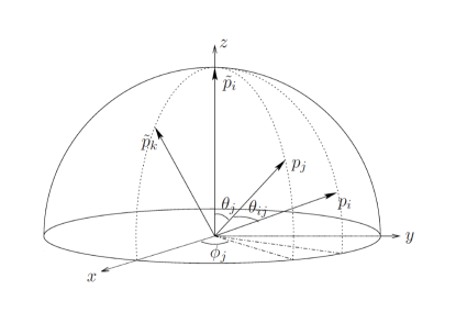
Figure 1: Parameterization of the angular variables for the final-state splitting $\tilde{p}_{i}\to p_{i}+p_{j}$. Here $\tilde{p}_{k}$ is the spectator parton selected to define the azimuthal variable $\phi_{j}$.

The phase space of the splitting has three degrees of freedom in $d=4$ dimensions. One possible way of parameterization is to use Lorentz-covariant scalar products and splitting variables as proposed in Ref. [40]. This simple choice results in compact formulae of the integrated dipoles for massless partons [41]. Applying the same strategy to the fully massive case, however, the kinematical bounds of the splitting become much more complicated and the resulting expressions turn out to be very cumbersome. To keep the final expressions reasonably compact, we have adopted an alternative parameterization. For example, in the case of the final-state emission, for a set of momenta $\{\tilde{p}\}_{m}$ the splitting $\tilde{p}_{i}\to p_{i}+p_{j}$ and the set of momenta $\{p\}_{m+1}$ had to be constructed out of three parameters that we have called collinear, soft and azimuthal variables. In the singular limit, where $P_{ij}^{2}\to m_{i}^{2}$, the collinear and the soft variables have to correspond to the relative angle between the nearly-collinear partons, $\theta_{ij}$, and the energy of the unresolved parton, $E_{j}$. On the other hand, the azimuthal variable, $\phi_{j}$, which is the second angular parameter uniquely fixes the kinematics of the splitting. Our reference frame consists of an orthogonal set of axes $(x,y,z)$, where the $z$-axis is identified with the spatial direction of the vector $\tilde{p}_{i}$, as shown in Figure 1. The azimuthal variable is then the angle, which separates the unresolved parton $p_{j}$ from the the $x$-$z$ plane. Since there is complete freedom in selecting the direction of the $x$-axis, we have decided to place it in the plane $\tilde{p}_{i}$-$\tilde{p}_{k}$, where $\tilde{p}_{k}$ is the momentum of the spectator. In the frame, where the total momentum $Q$ is at rest, the definition of the soft variable is as follows:

$$E_{j}\equiv\frac{\sqrt{Q^{2}}\,(P_{ij}^{2}-m_{i}^{2})}{P_{ij}^{2}-m_{i}^{2}+2\,\sqrt{Q^{2}}\,(\tilde{p}_{i}^{0}-\cos\theta_{j}\,|\vec{\tilde{p}}_{i}|)}\;.$$

It is convenient to divide this soft variable by its kinematically allowed maximum value to get a normalized soft variable $e$:

$$e\equiv E_{j}/E_{j}^{\rm max}\,.$$

The integration of the splitting phase space in case of the final-state emission runs over the variables

$$e\in[0,1]\;,$$

$$c\equiv\cos\theta_{j}\in[-1,1]\,,$$

$$\phi\equiv\phi_{j}\in[0,2\pi]\;.$$

The soft and collinear limits correspond to $e\to 0$ and $c\to 1$, respectively.

For the calculation of the integrated subtraction terms in the Nagy-Soper scheme, we have adopted the spin-averaged version of the splitting functions as described in Ref. [26]. Our goal is the integration in $d=4-2\epsilon$ dimensions over the whole phase space of the splitting. However, as a consequence of the increased complexity of the mapping, a fully analytic evaluation of the integrals turns out to be demanding. Thus, as an alternative we have used numerical approaches to integrate over the splitting phase space. More precisely, we have decided to adopt a semi-numerical approach to consider analytic integration when possible, and Monte Carlo integration otherwise. Since the general dependence of the integrands on the azimuthal variable $\phi$ was simple and all the azimuthal integrals could be classified into three groups, we carried out this part of the integration analytically. The dependence on the soft and collinear variables was not as simple and led to more complicated expressions that we treated numerically. Further details can be found in the original publication [38].

2.1 Implementation in Helac-Dipoles

We have incorporated the new subtraction method based on the Nagy-Soper formalism into the Helac-Dipoles package, preserving at the same time all the optimizations already available in the code. For a detailed description of the package functionalities, we refer to the existing literature [45, 46]. All elements of the calculation that do not dependent on a specific subtraction scheme, like the Born matrix elements and the color correlators, were already provided by the framework of Helac-Dipoles. This fact has dramatically simplified our implementation.

The construction of the Nagy-Soper subtraction terms is dictated by the form of the splitting functions. They contain generic spinors and polarization vectors, which enables them to treat simultaneously fixed helicities as well as random polarization states. We have provided random polarization sampling as a further option available for the Nagy-Soper scheme. This is an alternative to the existing random helicity sampling optimization, which uses stratified sampling over the different (incoherent) helicity assignments of partons [45]. The option for the spin sum treatment can be controlled by the user in the configuration file dipoles.conf as described in the Appendix of Ref. [46].

Besides random polarization sampling, which is an important speedup in every calculation, we have also provided random sampling over color, or color Monte Carlo, for the subtracted real radiation part. This functionality has provided an important speedup for matrix elements with a large number of colored external states. The general ideas from [47, 48] have been adopted, which are also an essential ingredient of the Helac-1Loop package [49].

Our implementation of the Nagy-Soper subtraction scheme (NS) has been tested and compared to the Catani-Seymour subtraction scheme (CS) for some specific processes. More precisely proton-proton collisions at the LHC with a center-of-mass energy of 8 TeV have been considered and the following partonic subprocesses $gg\to t\bar{t}b\bar{b}g$, $gg\to t\bar{t}t\bar{t}g$, $gg\to b\bar{b}b\bar{b}g$, $gg\to t\bar{t}ggg$ have been studied. They give dominant contributions to the subtracted real emissions at ${\cal O}(\alpha_{s}^{5})$ for the corresponding processes $pp\to t\bar{t}b\bar{b}+X$, $pp\to t\bar{t}t\bar{t}+X$, $pp\to b\bar{b}b\bar{b}+X$ and $pp\to t\bar{t}jj+X$. Moreover, they represent a high level of complexity and test almost all aspects of the software, as they involve both massive and massless states. We have imposed basic selection cuts on jets

$$p_{T}(j)>50~{}{\rm GeV},~{}~{}~{}~{}~{}~{}|y(j)|<2.5,~{}~{}~{}~{}~{}~{}\Delta R(jj)>1\,,$$

which have been defined through the anti-$k_{T}$ jet algorithm [50] with radius parameter $R=1$. The mass of the top quark was set to $m_{t}=173.5$ GeV and the bottom quark was considered to be massless. Results have been presented for the NLO CT10 parton distribution functions [51] with five active flavors and the corresponding two-loop $\alpha_{s}$. The renormalization and factorization scales were set to the scalar sum of the jet transverse masses

$$H_{T}=\sum_{i}m_{T}(j_{i})\,,$$

where for the top quark

$$m_{T}(t)=\sqrt{m_{t}^{2}+p^{2}_{T}(t)}$$

and for light jets (also tagged bottom-jets)

$$m_{T}(j)=p_{T}(j)\,.$$

A factor of $1/4$ has been included in the scales for all but the $gg\to b\bar{b}b\bar{b}g$ process where $\mu_{R}=\mu_{F}=H_{T}$ has been chosen instead.

In the following, a few examples from the comparison of both schemes are given. If not specified otherwise, full summation over all color configurations has been assumed together with random helicity sampling.

Process	Number of	Number of	Number of
	Dipoles (CS)	Dipoles (NS)	FD
$gg\to t\bar{t}b\bar{b}g$	55	11	341
$gg\to t\bar{t}t\bar{t}g$	30	6	682
$gg\to b\bar{b}b\bar{b}g$	90	18	682
$gg\to t\bar{t}ggg$	75	15	1240

Table 1: Number of Catani-Seymour (CS) and Nagy-Soper (NS) subtraction terms for dominant partonic subprocesses contributing to the subtracted real emission contributions at ${\cal O}(\alpha_{s}^{5})$ for the $pp\to t\bar{t}b\bar{b}+X$, $pp\to t\bar{t}t\bar{t}+X$, $pp\to b\bar{b}b\bar{b}+X$ and $pp\to t\bar{t}jj+X$ processes at the LHC. The number of Feynman diagrams (FD) corresponding to the subprocesses is given as well.

In Table 1, for example, the total number of subtraction terms that are evaluated in both schemes is shown. Also given is the number of Feynman diagrams corresponding to the subprocesses under scrutiny to underline their complexity. For each of the $2\to 5$ processes, five times less terms are needed in the NS subtraction scheme compared to the CS scheme. The difference corresponds to the total number of possible spectators, which are relevant in the CS case, but not in the NS case.

Process	$\sigma_{\rm RE}^{\rm CS}$ [pb]	$\sigma_{\rm RE}^{\rm NS}$ [pb]
$gg\to t\bar{t}b\bar{b}g$	$(28.39\pm 0.04)\cdot 10^{-3}$	$(28.59\pm 0.06)\cdot 10^{-3}$
$gg\to t\bar{t}t\bar{t}g$	$(16.98\pm 0.02)\cdot 10^{-5}$	$(17.01\pm 0.03)\cdot 10^{-5}$
$gg\to b\bar{b}b\bar{b}g$	$(66.24\pm 0.16)\cdot 10^{-2}$	$(66.06\pm 0.22)\cdot 10^{-2}$
$gg\to t\bar{t}ggg$	$(87.96\pm 0.07)\cdot 10^{-1}$	$(88.16\pm 0.08)\cdot 10^{-1}$

Table 2: Real emission cross sections for dominant partonic subprocesses contributing to the subtracted real emissions at ${\cal O}(\alpha_{s}^{5})$ for the $pp\to t\bar{t}b\bar{b}+X$, $pp\to t\bar{t}t\bar{t}+X$, $pp\to b\bar{b}b\bar{b}+X$ and $pp\to t\bar{t}jj+X$ processes at the LHC. Results are shown for two different subtraction schemes, the Catani-Seymour (CS) dipole subtraction and the new Nagy-Soper (NS) scheme, including the numerical error from the Monte Carlo integration.

Process	$t^{\rm CS}$ [msec]	$t^{\rm NS}$ [msec]	$t^{\rm RE}$ [msec]
$gg\to t\bar{t}b\bar{b}g$	$24.8$	$13.2$	$6.5$
$gg\to t\bar{t}t\bar{t}g$	$35.7$	$18.5$	$11.2$
$gg\to b\bar{b}b\bar{b}g$	$26.6$	$16.2$	$10.1$
$gg\to t\bar{t}ggg$	$214.8$	$108.2$	$48.7$

Table 3: The CPU time needed to evaluate the real emission matrix element together with all the subtraction terms for one phase space point for two subtraction schemes, namely Catani-Seymour, $t^{\rm CS}$, and Nagy-Soper, $t^{\rm NS}$. For comparison, we also give the CPU time for the pure real emission matrix element calculation, $t^{\rm RE}$. All numbers have been obtained on an Intel 3.40 GHz processor with the Intel Fortran compiler using the option -fast.

Process	$\sigma_{\rm RE,\,COL}^{\rm CS}$ [pb]	$\sigma_{\rm RE,\,COL}^{\rm NS}$ [pb]
$gg\to t\bar{t}b\bar{b}g$	$(28.35\pm 0.14)\cdot 10^{-3}$	$(28.77\pm 0.14)\cdot 10^{-3}$
$gg\to t\bar{t}t\bar{t}g$	$(17.00\pm 0.03)\cdot 10^{-5}$	$(17.01\pm 0.04)\cdot 10^{-5}$
$gg\to b\bar{b}b\bar{b}g$	$(65.71\pm 0.50)\cdot 10^{-2}$	$(67.00\pm 0.66)\cdot 10^{-2}$
$gg\to t\bar{t}ggg$	$(88.04\pm 0.37)\cdot 10^{-1}$	$(87.76\pm 0.31)\cdot 10^{-1}$

Table 4: Real emission cross sections for dominant partonic subprocesses contributing to the subtracted real emissions at ${\cal O}(\alpha_{s}^{5})$ for the $pp\to t\bar{t}b\bar{b}+X$, $pp\to t\bar{t}t\bar{t}+X$, $pp\to b\bar{b}b\bar{b}+X$ and $pp\to t\bar{t}jj+X$ processes at the LHC. Results are shown for random color sampling for two different subtraction schemes, the Catani-Seymour (CS) dipole subtraction and the new Nagy-Soper (NS) scheme, including the numerical error from the Monte Carlo integration.

Process	$\sigma_{\rm RE,\,POL}^{\rm NS}$ [pb]
$gg\to t\bar{t}b\bar{b}g$	$(28.50\pm 0.06)\cdot 10^{-3}$
$gg\to t\bar{t}t\bar{t}g$	$(17.01\pm 0.03)\cdot 10^{-5}$
$gg\to b\bar{b}b\bar{b}g$	$(66.23\pm 0.20)\cdot 10^{-2}$
$gg\to t\bar{t}ggg$	$(88.16\pm 0.07)\cdot 10^{-1}$

Table 5: Real emission cross sections for dominant partonic subprocesses contributing to the subtracted real emissions at ${\cal O}(\alpha_{s}^{5})$ for the $pp\to t\bar{t}b\bar{b}+X$, $pp\to t\bar{t}t\bar{t}+X$, $pp\to b\bar{b}b\bar{b}+X$ and $pp\to t\bar{t}jj+X$ processes at the LHC. Results are shown for random polarization sampling for the new Nagy-Soper (NS) subtraction scheme, including the numerical error from the Monte Carlo integration.

Real emission cross sections are presented in Table 2, again for the CS dipole subtraction and the new NS scheme. All results have been obtained with the same Monte Carlo statistics and the resulting relative errors are well below $1\%$. We observe that the difference between two evaluations of a given cross section is at most twice the sum of the corresponding errors. In Table 3, the time measured in milliseconds, needed to evaluate the real emission matrix element and the subtraction terms for one phase space point is shown. The NS is scheme is typically twice as fast as the CS scheme, but still a factor of about two slower than the evaluation of the real emission matrix element. Overall, both schemes, with their different momentum mappings and subtraction terms, show a comparable performance and give the same results for total real emission cross sections.

The performance of Monte Carlo sampling over color and polarization has also been studied. In Table 4 we present real emission cross sections, which have been evaluated with random color sampling, for both subtraction schemes. We observe agreement with the results presented in Table 2, where a summation over all color flows has been performed. One should note that in the case of the MC summation the absolute errors are $3-4$ times higher. In order to obtain the same absolute errors as for results including a summation of color flows, $9-16$ times more events need to be evaluated. However, the average number of color flows corresponding to a random color configuration, which is evaluated per phase space point, is dramatically reduced. The overall time to obtain the same result is therefore substantially shortened. Our conclusion is thus that random color sampling is a powerful approach, especially for processes where the number of gluons is higher and exceeds the number of quarks.

Finally, in Table 5 real emission cross sections for random polarization sampling for our new NS subtraction scheme are shown. They should be compared to the numbers given in Table 2, where we have used random helicity sampling. Perfect agreement is found.

To conclude this section, a complete implementation of the Nagy-Soper subtraction scheme both for massive and massless partons is now available in the Helac-Dipoles software. By design, the Nagy-Soper scheme has less kinematical mappings and is, therefore, faster. On the other hand, we have observed that the absolute error of the most costly (in terms of computational time) subtracted real emission contribution was slightly worse for Nagy-Soper than for Catani-Seymour. In the end, we conclude that both schemes are similar in terms of efficiency. We did not consider differences below a factor of two in error or time, which are moreover process dependent, a reason to prefer either scheme. There are two advantages of our implementation: First, we can now perform better tests when calculating fixed order NLO QCD corrections by computing real radiation in two different schemes. A case study is described in the next section. Second, the integrated subtraction terms facilitate the matching of the fixed order calculation and the Nagy-Soper parton shower with quantum interference. This part is described in Section 4.

3 A case study: NLO-QCD corrections to the production of four bottom quarks at the LHC

The production of four bottom quarks, $pp\to b\bar{b}b\bar{b}+X$, is an important background to various Higgs analyses and new physics searches at the LHC, including for example Higgs-boson pair production in two-Higgs doublet models at large $\tan\beta$ [52], or so-called hidden valley scenarios where additional gauge bosons can decay into bottom quarks [53]. Accurate theoretical predictions for the Standard Model production of multiple bottom quarks are thus mandatory to exploit the potential of the LHC for new physics searches. Furthermore, the calculation of the NLO QCD corrections to $pp\to b\bar{b}b\bar{b}+X$ provides a substantial technical challenge and requires the development of efficient techniques, with a high degree of automation. In Ref. [54] we have performed an NLO calculation of $b\bar{b}b\bar{b}$ production at the LHC with the Helac-NLO system [46]. In particular, we have presented results based on the Nagy-Soper subtraction scheme introduced in Section 2. Two calculational schemes have been employed, the so-called four-flavor scheme (4FS) with only gluons and light-flavor quarks in the proton, where massive bottom quarks are produced from gluon splitting at short distances, and the five-flavor-scheme (5FS) [55] with massless bottom quarks as partons in the proton. At all orders in perturbation theory, the four- and five-flavor schemes are identical, but the way of ordering the perturbative expansion is different, and at any finite order the results do not match. Comparing the predictions of the two schemes at NLO thus provides a way to assess the theoretical uncertainty from unknown higher-order corrections, and to study the effect of the bottom mass on the inclusive cross section and on differential distributions. First NLO results for $pp\to b\bar{b}b\bar{b}+X$ in the 5FS have been presented in Ref. [56]. In Ref. [54] we have not only provided an independent calculation of this challenging process with a different set of methods and tools, but also a systematic study of the bottom quark mass effects by comparing the 5FS and 4FS results. We note that NLO results for the production of four top quarks in hadron collisions have been discussed in Ref. [57].

The calculation of the process $pp\to b\bar{b}b\bar{b}+X$ at NLO QCD comprises the parton processes $gg\to b\bar{b}b\bar{b}$ and $q\bar{q}\to b\bar{b}b\bar{b}$ at tree-level and including one-loop corrections, as well as the tree-level parton processes $gg\to b\bar{b}b\bar{b}+g$, $q\bar{q}\to b\bar{b}b\bar{b}+g$, $gq\to b\bar{b}b\bar{b}+q$ and $g\bar{q}\to b\bar{b}b\bar{b}+\bar{q}$. In the four-flavor scheme $q\in\{u,d,c,s\}$, and the bottom quark is treated massive. The bottom mass effects are in general suppressed by powers of $m_{b}/\mu$, where $\mu$ is the hard scale of the process, e.g. the transverse momentum of a bottom-jet. Potentially large logarithmic corrections $\propto\ln(m_{b}/\mu)$ could arise from nearly collinear splitting of initial-state gluons into bottom quarks, $g\to b\bar{b}$, where the bottom mass acts as a regulator of the collinear singularity. This class of $\ln(m_{b}/\mu)$-terms can be summed to all orders in perturbation theory by introducing bottom parton densities in the five-flavor scheme. The 5FS is based on the approximation that the bottom quarks from the gluon splitting are produced at small transverse momentum. However, in our calculation we have required that all four bottom quarks can be experimentally detected, and we have thus imposed a lower cut on the bottom transverse momentum, $p_{T,b}\geq p_{T,b}^{\rm min}$. As a result, up to NLO accuracy the potentially large logarithms in the process $pp\to b\bar{b}b\bar{b}+X$ are replaced by $\ln(m_{b}/\mu)\to\ln(p_{T,b}^{\rm min}/\mu)$, with $m_{b}\ll p_{T,b}^{\rm min}\lesssim\mu$, and are thus much less significant numerically. Therefore, for the process at hand, the differences between the 4FS and 5FS calculations with massive and massless bottom quarks, respectively, should be moderate, but may not be completely negligible.

Our calculation has been performed with the automated Helac-NLO framework [46], which includes Helac-1loop [49] for the evaluation of the numerators of the loop integrals and the rational terms, CutTools [58], which implements the OPP reduction method [59, 60, 61, 62] to compute one-loop amplitudes, and OneLoop [63] for the evaluation of the scalar integrals. The singularities for soft and collinear parton emission are treated using subtraction schemes as implemented in Helac-Dipoles [45], see the discussion in Section 2. The phase space integration is performed with the help of the Monte Carlo generators Helac-Phegas [64, 65, 66] and Kaleu [67], including Parni [68] for the importance sampling.

The Helac-Dipoles package has been based on the standard Catani-Seymour dipole subtraction formalism [43, 44]. We have extended Helac-Dipoles by implementing the new subtraction scheme [40, 41] based on the momentum mapping and the splitting functions derived in the context of an improved parton shower formulation by Nagy and Soper [23], as described in Section 2. The results presented in Ref. [54] have been the first application of the Nagy-Soper subtraction scheme for a $2\to 4$ scattering process with massive and massless fermions.

Below we shall present a number of selected numerical results for the $pp\to b\bar{b}b\bar{b}+X$ cross section at the LHC at the centre-of-mass energy of ${\sqrt{s}=14}$ TeV. We discuss the impact of the NLO-QCD corrections, and study the dependence of the results on the bottom quark mass.

Let us first specify the input parameters and the acceptance cuts we impose. The top quark mass, which appears in the loop corrections, is set to $m_{t}=173.5$ GeV [69]. We combine collinear final-state partons with pseudo-rapidity $|\eta|<5$ into jets according to the anti-$k_{T}$ algorithm [50] with separation $R=0.4$. The bottom-jets have to pass the transverse momentum and rapidity cuts $p_{T,b}>30$ GeV and $|y_{b}|<2.5$, respectively. The renormalisation and factorisation scales are set to the scalar sum of the bottom-jet transverse masses, $\mu_{R}=\mu_{F}=\mu_{0}=H_{T}$, with

$$H_{T}=m_{T,b}+m_{T,\bar{b}}+m_{T,b}+m_{T,\bar{b}}$$

and the transverse mass

$$m_{T,b}=\sqrt{m^{2}_{b}+p^{2}_{T,b}}\,.$$

For the five-flavor scheme calculation with massless bottom quarks the transverse mass equals the transverse momentum, $m_{T,b}=p_{T,b}$. Note that the implementation of a dynamical scale requires a certain amount of care, as the subtraction terms for real radiation have to be evaluated with a different kinematical configuration specified by the momentum mapping of the subtraction scheme. Comparing the results as obtained with the Catani-Seymour subtraction and the Nagy-Soper scheme, which is based on a different momentum mapping, provides an important and highly non-trivial internal check of the calculation.

3.1 Massless bottom quarks within the five-flavor scheme

The NLO predictions for the inclusive cross section are presented in Table 6 for the NLO MSTW2008 [70] parton distribution function (pdf), with five active flavors and the corresponding two-loop $\alpha_{\rm s}$. To study the impact of the higher-order corrections, we also show leading-order results obtained using the MSTW2008 LO pdf sets and one-loop running for $\alpha_{\rm s}$.

Varying the renormalisation and factorisation scales simultaneously about the central scale by a factor of two, we find a residual scale uncertainty of approximately 30% at NLO, a reduction by about a factor of two compared to LO. The $K$-factor, $K=\sigma_{\rm NLO}/\sigma_{\rm LO}=1.37$, is sizeable. Note, however, that the $K$-factor is an unphysical quantity and depends strongly on both the default choice of scale and the pdf set [54].

In Ref. [54] we have also presented predictions for selected differential distributions which are an important input for the experimental analyses and the interpretation of the experimental data. Figure 2 shows LO and NLO predictions for the transverse momentum of the hardest bottom jet. We also show the theoretical uncertainty through scale variation and the $K$-factor as a function of the transverse momentum. It is evident from Figure 2 that the NLO corrections significantly reduce the theoretical uncertainty of the differential distributions, and that the size of the higher-order effects depends on the kinematics. For an accurate description of exclusive observables and differential distributions it is thus not sufficient to rescale the LO prediction with an inclusive $K$-factor.

$pp\to b\bar{b}b\bar{b}+X$	$\sigma_{\rm LO}$ [pb]	$\sigma_{\rm NLO}$ [pb]	$K=\sigma_{\rm NLO}/\sigma_{\rm LO}$
5FS	$99.9^{+58.7\,(59\%)}_{-34.9\,(35\%)}$	$136.7^{+38.8(28\%)}_{-30.9\,(23\%)}$	1.37
4FS	$84.5^{+49.7(59\%)}_{-29.6(35\%)}$	$118.3^{+33.3(28\%)}_{-29.0(24\%)}$	1.40

Table 6: 5FS and 4FS LO/NLO cross sections for $pp\rightarrow b\bar{b}b\bar{b}~{}+X$ at the LHC ($\sqrt{s}$ = 14 TeV). The renormalisation and factorisation scales have been set to the central value $\mu_{0}=H_{T}$, and the uncertainty is estimated by varying both scales simultaneously by a factor two about the central scale. Results are shown for the 5FS/4FS MSTW2008LO/NLO pdf sets.

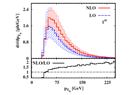
Figure 2: Differential cross section for $pp\rightarrow b\bar{b}b\bar{b}~{}+X$ at the LHC ($\sqrt{s}$ = 14 TeV) in the 5FS as a function of the transverse momentum of the hardest bottom jet. The dash-dotted (blue) curve corresponds to the LO and the solid (red) curve to the NLO result. The scale choice is $\mu_{R}=\mu_{F}=\mu_{0}=H_{T}$. The hashed area represents the scale uncertainty, and the lower panels display the differential K factor. The cross sections are evaluated with the MSTW2008 pdf sets.

3.2 Massive bottom quarks within the four-flavor scheme

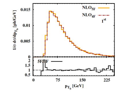
Figure 3: Differential cross section for $pp\rightarrow b\bar{b}b\bar{b}~{}+X$ at the LHC ($\sqrt{s}$ = 14 TeV) in the 4FS and 5FS as a function of the transverse momentum of the hardest bottom jet, normalised to the corresponding inclusive cross section. The scale choice is $\mu_{R}=\mu_{F}=\mu_{0}=H_{T}$, the cross sections are evaluated with the 5FS and 4FS MSTW2008 pdf sets, respectively.

Within the four-flavor scheme, bottom quarks are treated massive and are not included in the parton distribution functions of the proton. We define the bottom quark mass in the on-shell scheme and use $m_{b}=4.75$ GeV, consistent with the choice made in the MSTW2008 four-flavor pdf [71].

The central cross section predictions in LO and NLO for $\mu=H_{T}$ using the 4FS MSTW2008 [71] pdf are shown in Table 6, in comparison with the 5FS results. We observe that the bottom mass effects decrease the cross section prediction by $18\%$ at LO and $16\%$ at NLO. The residual scale dependence at NLO is approximately 30%, similar to the 5FS calculation.

The difference between the massless 5FS and the massive 4FS calculations has two origins. First, there are genuine bottom mass effects, the size of which depends sensitively on the transverse momentum cut. For $p_{T,b}^{\rm min}=30$ GeV we find a 10% difference between the 5FS and 4FS from non-singular bottom-mass dependent terms. This difference decreases to about $1\%$ for $p_{T,b}^{\rm min}=100$ GeV. Second, the two calculations involve different pdf sets and different corresponding $\alpha_{\rm s}$. While a 4FS pdf has, in general, a larger gluon flux than a 5FS pdf, as there is no $g\to b\bar{b}$ splitting, the corresponding four-flavor $\alpha_{\rm s}$ is smaller than for five active flavors. For $pp\rightarrow b\bar{b}b\bar{b}~{}+X$ the difference in $\alpha_{\rm s}$ is prevailing and results in a further reduction of the 4FS cross section prediction by about $5\%$. This latter difference should be viewed as a scheme dependence rather than a bottom mass effect.

In Figure 3 we present the differential distribution in the transverse momentum of the hardest bottom jet, as calculated in the 5FS with massless bottom quarks and in the 4FS with $m_{b}=4.75$ GeV, normalised to the corresponding inclusive cross section. We find that the difference in the shape of the distributions in the 5FS and the 4FS is very small.

To conclude this section, we have presented selected results for the differential cross-sections for $pp\to b\bar{b}b\bar{b}+X$ at the LHC at the centre-of-mass energy of ${\sqrt{s}=14}$ TeV [54]. We find that the higher-order corrections significantly reduce the scale dependence, with a residual theoretical uncertainty of about 30% at NLO. The impact of the bottom quark mass is moderate for the cross section normalisation and negligible for the shape of distributions. The fully differential NLO cross section calculation for the process $pp\rightarrow b\bar{b}b\bar{b}~{}+X$ presented in Ref. [54] provides an important input for the experimental analyses and the interpretation of new physics searches at the LHC.

4 Parton shower with quantum interference and matching

In this section, we will discuss the Nagy-Soper shower in more detail, including its particular implementation in the C++ library Deductor [35]. Among other topics, we will elaborate on the theoretical framework necessary to include quantum interference effects. Furthermore, we will point out the inherent ambiguities of the approach. Ultimately, we will discuss the matching to fixed order calculations at the next-to-leading order in QCD, and present some results for a non-trivial process: the production of a top-anti-top-quark pair in association with a jet in hadronic collisions. This section is based on [72].

4.1 Basic concepts

We start from a generic $2\to m$ process, which is defined by two initial state partons $a$ and $b$ and $1,...,m$ final state particles. Each particle is described by a set of quantum numbers to define the flavor $f_{i}$, spin $s_{i}$ and color $c_{i}$ of the particle and its momentum $p_{i}$. The initial state parton kinematics is described by momentum fractions, $\eta_{a}$ and $\eta_{b}$, with respect to the original colliding hadrons, instead of their momenta. Thus, a complete parton ensemble can be described by

$$\{p,f,s,c\}_{m}\equiv\{[\eta_{a},-f_{a},s_{a},c_{a}],[\eta_{b},-f_{b},s_{b},c_{b}],\\ [p_{1},f_{1},s_{1},c_{1}],...,[p_{m},f_{m},s_{m},c_{m}]\}\;.$$

The state of the parton shower evolution is described by a quantum density matrix $\rho$, which gives the ’probability’ to find a certain parton ensemble $\{p,f,s,c\}_{m}$. The expectation value of an observable $F$ for any final state multiplicity is given by

$$\begin{split}\sigma[F]=&\sum_{m}\frac{1}{m!}\int[d\{p,f\}_{m}]\frac{f_{a}(\eta_{a},\mu_{F}^{2})f_{b}(\eta_{b},\mu_{F}^{2})}{4n_{c}(a)n_{c}(b)\times\text{flux}}\\ &\quad\quad\quad\times\bra{M(\{p,f\}_{m})}F(\{p,f\}_{m})\ket{M(\{p,f\}_{m})}\\ =&\sum_{m}\frac{1}{m!}\int[d\{p,f\}_{m}]Tr[\rho(\{p,f\}_{m})F(\{p,f\}_{m})]\;.\end{split}$$

Here the $1/m!$ is the symmetry factor for identical particles in the final state and $[d\{p,f\}_{m}]$ is the $m$ particle phase space measure. $f_{a/b}(\eta,\mu_{F}^{2})$ are the parton density functions evaluated at the momentum fraction $\eta$ and factorization scale $\mu_{F}^{2}$. The factor $4$ in the denominator is the spin averaging factor. $n_{c}(i)$ represents the averaging color factor for the initial state partons, where $n_{c}(q)=3$ and $n_{c}(g)=8$. The expectation value of F and the trace in the second line are meant to be a summation over indices in color $\otimes$ spin space. The quantum density $\rho$ introduced in the second line, is thus given by

$$\begin{split}\rho(\{p,f\}_{m})&=\;\frac{f_{a}(\eta_{a},\mu_{F}^{2})f_{b}(\eta_{b},\mu_{F}^{2})}{4n_{c}(a)n_{c}(b)\times\text{flux}}\\ &\times\ket{M(\{p,f\}_{m})}\bra{M(\{p,f\}_{m})}\\ &=\sum_{s,c}\sum_{s^{\prime},c^{\prime}}\ket{\{s,c\}_{m}}\rho(\{p,f,s^{\prime},c^{\prime},s,c\}_{m})\bra{\{s^{\prime},c^{\prime}\}_{m}}\;.\end{split}$$ (1)

It is useful to define basis vectors $|\{p,f,s^{\prime},c^{\prime},s,c\}_{m})$, such that

$$\rho(\{p,f,s^{\prime},c^{\prime},s,c\}_{m})=(\{p,f,s^{\prime},c^{\prime},s,c\}_{m}|\rho)\;.$$

One can then write the expectation value of the observable $F$ as

$$\sigma[F]=(F|\rho)\;.$$

A particularly important observable for the defintion of the parton shower is the total cross section measurement function. It is defined as

$$(1|\{p,f,s^{\prime},c^{\prime},s,c\}_{m})=\braket{\{s^{\prime}\}_{m}}{\{s\}_{m}}\braket{\{c^{\prime}\}_{m}}{\{c\}_{m}}\;.$$

The shower evolution equation describes the propagation of the quantum density matrix from some initial shower “time”, $t_{0}$, which represents the hard interaction, to the final “time” $t_{F}$ in the low energy regime. The final shower time $t_{F}$ characterizes the physical scale at which parton emissions cannot be described perturbatively anymore. The definition of shower time $t$ is not unique and is explained later. The parton shower evolution will transform a few partons at the matrix element level, to a realistic final state with jets typically made of many partons. After this evolution, a phenomenological hadronization model must be applied. The perturbative evolution itself is described by a unitary operator $U(t_{F},t_{0})$. The observable $F$, after showering, has the expectation value

$$\sigma[F]=(F|\rho(t_{F}))=(F|U(t_{F},t_{0})|\rho(t_{0}))\;.$$

The unitarity of the evolution operator is a consequence of the requirement that it should not change the total cross section. Thus $(1|U(t_{F},t_{0})|\rho(t_{0}))=(1|\rho(t_{0}))$. The evolution operator can be obtained from a differential equation involving two operators $\mathcal{H}_{I}(t)$ and $\mathcal{V}(t)$, corresponding to the concepts of real and virtual corrections respectively:

$$\frac{dU(t,t_{0})}{dt}=[\mathcal{H}_{I}(t)-\mathcal{V}(t)]U(t,t_{0})\;.$$ (2)

Here $\mathcal{H}_{I}(t)$ describes the emission of a resolved particle, i.e. the momenta, flavor, spins and color configuration will change after its application. $\mathcal{V}(t)$ describes the unresolved emission and therefore does not alter momentum or flavor configurations. Nevertheless it can change color configurations, which will affect further emissions. For convenience of calculations, the virtual operator can be further decomposed into $\mathcal{V}(t)=\mathcal{V}_{E}(t)+\mathcal{V}_{S}(t)$, where $\mathcal{V}_{E}(t)$ is diagonal in color space, while $\mathcal{V}_{S}(t)$ is not. Interestingly, the evolution equation takes the same form as the time evolution of a statistical ensemble in Liouville space

$$\frac{\partial\rho(t)}{\partial t}=\frac{i}{\hbar}[\rho(t),H]=L\rho(t)\;,$$

where the Liouville operator can be identified as $L=[\mathcal{H}_{I}(t)-\mathcal{V}(t)]$.

Traditional parton showers are constructed using the large $N_{c}$ limit. Thus, the state is always color diagonal implying $\mathcal{V}_{S}(t)\to 0$. In this case, Eq. (2) yields

$$U(t,t_{0})=N(t,t_{0})+\int_{t_{0}}^{t}d\tau~{}U(t,\tau)\mathcal{H}_{I}(\tau)N(\tau,t_{0})\;,$$

with the Sudakov form factor

$$N(t,t_{0})=\mathbb{T}\exp\left(-\int_{t_{0}}^{t}d\tau~{}\mathcal{V}(\tau)\right)\;.$$

Since $\mathcal{V}(t)$ is diagonal in the traditional approach, $N(t,t_{0})$ is a number and not a matrix in color space. In the general case with non-diagonal $\mathcal{V}(t)$, it is not practical to exponentiate a matrix in color space. The idea is, therefore, to exponentiate only the diagonal color part $\mathcal{V}_{E}(t)$, and treat $\mathcal{V}_{S}(t)$ iteratively as a perturbation. This can be justified by noting that the off diagonal color contributions are always suppressed by a relative factor of $1/N_{c}^{2}$ compared to the leading color contributions. Therefore, the solution of Eq. (2) with full color evolution, using the decomposition of $\mathcal{V}(t)=\mathcal{V}_{E}(t)+\mathcal{V}_{S}(t)$, is given by

$$U(t,t_{0})=N(t,t_{0})\\ +\int_{t_{0}}^{t}d\tau~{}U(t,\tau)\left[\mathcal{H}_{I}(\tau)-\mathcal{V}_{S}(\tau)\right]N(\tau,t_{0})\;.$$

with

$$N(t,t_{0})=\mathbb{T}\exp\left(-\int_{t_{0}}^{t}d\tau~{}\mathcal{V}_{E}(\tau)\right)\;.$$

4.2 Real and virtual evolution operators

The real evolution operator, $\mathcal{H}_{I}$, describes the transition from an $m$-particle ensemble to an $(m+1)$-particle ensemble. This is achieved by splitting a chosen parton into two, which would physically correspond to a decay of a slightly off-shell parton. The splitting is constrained by flavor conservation, $f_{l}\to\hat{f}_{l}+\hat{f}_{m+1}$, and momentum conservation, $p_{l}\to\hat{p}_{l}+\hat{p}_{m+1}$. The description of the transition is ambiguous, as only the singular limits of amplitudes are uniquely determined in QCD. After emitting a particle, it is necessary to correct the momenta in the event in order to ensure momentum conservation and preserve the on-shellness of all particles. This is done by certain momentum mapping operators, which define momenta and flavors of the new ensemble

$$\{\hat{p},\hat{f}\}_{m+1}=R_{l}(\{p,f\}_{m})\;.$$ (3)

where $l\in\{a,b,1,...,m\}$. In Deductor, a global momentum mapping has been chosen. Whenever a particle is emitted, the momentum of all final state particles is affected, see the discussion in Section 2. In contrast, e.g. the Sherpa [19] parton shower is based on Catani-Seymour dipoles [43], which have local momentum mappings. In this case a single parton momentum is modified. An explicit description of the original momentum mapping used in Deductor can be found either in Ref. [23] or in Ref. [38]. Recently, the initial state momentum mapping has been slightly modified. A study [31] showed, that the generated $p_{T}$ spectrum in $pp\to Z$ strongly depends on the momentum mapping for initial state parton splittings. For this reason, Deductor uses a momentum mapping, which allows for an improved resummation of higher-order corrections [36].

Besides momentum and flavor mapping operators, $\mathcal{H}_{I}(t)$ contains splitting functions which correspond to the factorisation of amplitudes in the soft, collinear and soft-collinear limits. In these limits the amplitude can be written as

$$\ket{M(\{\hat{p},\hat{f}\}_{m+1})}=v(\{\hat{p},\hat{f}\}_{m+1})\ket{M(\{p,f\}_{m})}\;.$$

The operator $v(\{\hat{p},\hat{f}\}_{m+1})$ acts in color and spin space. The behaviour of amplitudes in singular limits translates into a similar behaviour of the density matrix, which can be written more explicitly as

$$\begin{split}\rho(\{\hat{p},&\hat{f}\}_{m+1})\sim\\ &\sum_{l,k}T_{l}^{\dagger}(f_{l}\to\hat{f}_{l}+\hat{f}_{m+1})V_{l}^{\dagger}(\{\hat{p},\hat{f}\}_{m+1})\rho(\{p,f\}_{m})\\ &\times V_{k}(\{\hat{p},\hat{f}\}_{m+1})T_{k}(f_{k}\to\hat{f}_{k}+\hat{f}_{m+1})\;,\end{split}$$ (4)

where $T_{l}^{\dagger}(f_{l}\to\hat{f}_{l}+\hat{f}_{m+1})$ is an operator in color space, while $V_{l}^{\dagger}(\{\hat{p},\hat{f}\}_{m+1})$ is an splitting operator in spin space. The general prescription to obtain Deductor’s splitting functions $V_{l}$ has been summarised in [38], whereas the complete set of splitting functions can be found in [23].

The approximation in Eq. (4) can be cast into an operator equation, $|\rho_{m+1})=\sum_{l}\mathcal{S}_{l}|\rho_{m})$. The operator $\mathcal{S}_{l}$ describes all possible splittings of the emitter parton $l$. $\mathcal{H}_{I}(t)$ is then defined by the splitting operators $\mathcal{S}_{l}$ at a fixed shower time $\mathcal{T}_{l}(\{p,f\}_{m}$

$$\mathcal{H}_{I}(t)=\sum_{l}\mathcal{S}_{l}\delta\left(t-\mathcal{T}_{l}(\{p,f\}_{m})\right)\;,$$ (5)

where the sum runs over all possible emitters $l$. The shower time $\mathcal{T}_{l}(\{p,f\}_{m})$ corresponds to an infrared sensitive scale, discussed in Section 4.4.

The virtual evolution operator, $\mathcal{V}(t)$, represents the unresolved virtual corrections. Nevertheless its content is fixed due to the unitarity condition of the parton shower. By applying $(1|$ from the left and $|\rho)$ from the right to Eq. (2) one obtains

$$(1|\mathcal{H}_{I}(t)-\mathcal{V}(t)|\rho(t))=0\;,$$

which should be valid for any $|\rho(t))$. Parton shower unitarity corresponds to simplified virtual corrections, whose main function is to cancel the divergences of the real corrections. In order to obtain an expression for $\mathcal{V}(t)$, we write

$$(1|\mathcal{V}(t)|\{p,f,c^{\prime},c,s^{\prime},s\}_{m})=(1|\mathcal{H}_{I}(t)|\{p,f,c^{\prime},c,s^{\prime},s\}_{m})\;.$$

This equation has an ambiguous solution in color space. We shall not reproduce here the explicit form for $\mathcal{V}(t)$ used in Deductor. It can be found in [23].

4.3 Logarithmic accuracy

In the previous section, we discussed the real and virtual evolution operators. While they allow for an exact treatment of color, the current implementation of Deductor is based on the so-called LC+ approximation [32], which amounts to only allowing for color evolution without non-local modifications of the color state. In this case, we identify $\mathcal{V}_{E}(t)=\mathcal{V}^{\rm LC+}(t)$ and $\mathcal{V}_{S}(t)=\Delta\mathcal{V}(t)=\mathcal{V}(t)-\mathcal{V}^{\rm LC+}(t)$.

The color diagonal part of the virtual operator will be exponentiated, which yields a parton shower formulation similar to the traditional one. The evolution equation is given by

$$U^{\rm LC+}(t,t_{0})=N^{\rm LC+}(t,t_{0})+\\ \int_{t_{0}}^{t}d\tau~{}U^{\rm LC+}(t,\tau)\mathcal{H}_{I}^{\rm LC+}(\tau)N^{\rm LC+}(\tau,t_{0})\;,$$

where

$$N^{\rm LC+}(t,t_{0})=\exp\left(-\int_{t_{0}}^{t}d\tau~{}\mathcal{V}^{\rm LC+}(\tau)\right)\;.$$

The color off-diagonal splittings are included perturbatively

$$U(t,t_{0})=U^{\rm LC+}(t,t_{0})+\\ \int_{t_{0}}^{t}d\tau~{}U(t,\tau)\left[\Delta\mathcal{H}_{I}(\tau)-\Delta\mathcal{V}(\tau)\right]U^{\rm LC+}(\tau,t_{0})\;,$$ (6)

where $\Delta\mathcal{H}_{I}(t)=\mathcal{H}_{I}(t)-\mathcal{H}_{I}^{\rm LC+}(t)$ and $\Delta\mathcal{V}(t)=\mathcal{V}(t)-\mathcal{V}^{\rm LC+}(t)$.

Let us investigate the logarithmic accuracy of observables. We suppose that the parton shower is used to calculate an observable $\mathcal{O}$ which contains large logarithms L of some invariant. For definiteness, we could image this invariant to be the transverse momentum of a gauge boson. Then $\langle\mathcal{O}\rangle$ has the form

$$\langle\mathcal{O}\rangle=\sum_{n}c(n,2n)\alpha_{s}^{n}L^{2n}+\sum_{n}c(n,2n-1)\alpha_{s}^{n}L^{2n-1}+\cdots.$$

We further suppose that a shower with full color, generated by $U(t,t_{0})$ reproduces all coefficients $c(n,2n)$ and $c(n,2n-1)$ correctly. Then $U^{\rm LC+}(t,t_{0})$ will reproduce $c(n,2n)$ exactly, because the LC+ approximation is exact with respect to the soft-collinear singularities. One insertion of $\left[\Delta\mathcal{H}_{I}(\tau)-\Delta\mathcal{V}(\tau)\right]$ generates a contribution $\sim\alpha_{s}L$ because it contains a correction for soft wide-angle gluon emission. This term multiplies contributions of order $\alpha_{s}^{n-1}L^{2n-2}$ and, therefore, corrects the coefficient $c(n,2n-1)$. A second insertion of $\left[\Delta\mathcal{H}_{I}(\tau)-\Delta\mathcal{V}(\tau)\right]$ would only affect the coefficients $c(n,j\leq 2n-2)$. Therefore, one insertion is sufficient to obtain NLL accuracy [32]. (An illustration of the logarithm counting is given in Figure 4.) This implies that NLL accuracy is in fact obtained with the evolution equation

$$U(t,t_{0})=U^{\rm LC+}(t,t_{0})+\\ \int_{t_{0}}^{t}d\tau~{}U^{\rm LC+}(t,\tau)\left[\Delta\mathcal{H}_{I}(\tau)-\Delta\mathcal{V}(\tau)\right]U^{\rm LC+}(\tau,t_{0})\;.$$

Figure 4: Illustration of the logarithm counting. One step in the vertical direction is given by an insertion of $U^{\rm LC+}$ and a diagonal step is given by an insertion of $\Delta\mathcal{H}_{I}(t)-\Delta\mathcal{V}(t)$. One can see, that two insertions of $\Delta\mathcal{H}_{I}(t)-\Delta\mathcal{V}(t)$ only contribute to the coefficient of $\alpha_{s}^{n}L^{2n-2}$.

4.4 Shower time

Emissions generated by a parton shower are strongly ordered in some kinematic variable in order to correctly resum the leading logarithms. It turns out that the choice of the ordering variable, which we call shower time, is ambiguous. The essential approximation made in the parton shower description is that, in each step of the evolution, all partons are on-shell. Thus, the parton shower time should allow us to neglect the virtuality of a splitting parton. Here, we summarize the discussion from Ref. [36] for final state radiation. The discussion for initial state radiation is analogous.

Consider a mother parton $0$ which splits in two partons, $p_{0}\to p_{1}+p_{2}$. The momentum $p_{0}$ is given in light-cone variables $(+,-,\perp)$, where $\vec{p}_{0}$ denotes the transverse momentum. We denote the virtuality of the parton as $v_{0}^{2}$. The momentum takes the form

$$p_{0}=\left(P,\frac{\vec{p}^{~{}2}_{0}+m_{0}^{2}+v_{0}^{2}}{2P},\vec{p}_{0}\right)\;.$$

The daughter momenta are given in the Sudakov parameterisation as

$$p_{1} =\left(zP,\frac{\vec{p}^{~{}2}_{1}+m_{1}^{2}+v_{1}^{2}}{2zP},\vec{p}_{1}\right)\;,$$

$$p_{2} =\left((1-z)P,\frac{\vec{p}^{~{}2}_{2}+m_{2}^{2}+v_{2}^{2}}{2(1-z)P},\vec{p}_{2}\right)\;.$$

From momentum conservation we obtain

$$v_{0}^{2}=\frac{((1-z)\vec{p}_{1}-z\vec{p}_{2})^{2}}{z(1-z)}+\frac{m_{1}^{2}}{z}+\frac{m_{2}^{2}}{1-z}-m_{0}^{2}+\frac{v_{1}^{2}}{z}+\frac{v_{2}^{2}}{1-z}\;.$$

In order to be allowed to neglect $v_{1}^{2}$ and $v_{2}^{2}$ at each step of the evolution, we must require

$$\frac{v_{1}^{2}}{z}\ll v_{0}^{2}\;,\qquad\frac{v_{2}^{2}}{1-z}\ll v_{0}^{2}\;.$$

Inserting the momentum fraction $z$

$$z=\frac{p_{1}\cdot Q_{0}}{p_{0}\cdot Q_{0}}\;,$$

$$1-z=\frac{(p_{0}-p_{1})\cdot Q_{0}}{p_{0}\cdot Q_{0}}\approx\frac{p_{2}\cdot Q_{0}}{p_{0}\cdot Q_{0}}\;,$$

where the last approximation is valid in the singular limit $p_{0}\approx p_{1}+p_{2}$. Here, $Q_{0}$ is the total final state momentum. We finally arrive at the conditions

$$\frac{v_{1}^{2}}{2p_{1}\cdot Q_{0}}\ll\frac{v_{0}^{2}}{2p_{0}\cdot Q_{0}}\quad\text{ and }\quad\frac{v_{2}^{2}}{2p_{2}\cdot Q_{0}}\ll\frac{v_{0}^{2}}{2p_{0}\cdot Q_{0}}\;.$$

They should always be fulfilled. Therefore, we define

$$\Lambda^{2}_{l}=\frac{|(\hat{p}_{l}\pm\hat{p}_{m+1})^{2}-m^{2}_{l}|}{2p_{l}\cdot Q_{0}}Q_{0}^{2}\;,$$

and enforce the emissions to be ordered in $\Lambda^{2}_{l}$. This can be achieved by defining the dimensionless shower time as

$$\mathcal{T}_{l}(\{p,f\}_{m})=-\log\left(\frac{\Lambda_{l}^{2}}{Q_{0}^{2}}\right)\;.$$

Generally, one can choose other ordering variables. E.g. Pythia 8 [73] uses the transverse momentum, $p_{T}$, in the parton splittings to order the emissions, Herwig [74, 75] uses angualar ordering, and Pythia 6 [76] uses a virtuality ordering. A consequence of the $\Lambda^{2}$ ordering is an enlarged phase space for initial state splittings as compared to $p_{T}$ ordering [36].

4.5 Ambiguities of the parton shower definition

As we have already pointed out at various places, the construction of the parton shower is not uniquely defined. In the following we list the main ambiguities. They should be kept in mind, since future findings might require modifications of their solutions.

Momentum Mappings:

The way the parton shower distributes momentum among the particles after splitting may influence the resummation accuracy. In case of Drell-Yan Z-boson production, a study [31] showed that a different momentum mapping [36] generates a different $p_{T}$ spectrum of the Z-Boson.

Splitting functions:

Splitting functions are only required to reproduce the singular limits of QCD matrix elements, but can have an arbitrary finite remainder.

Soft partition function:

Soft emissions are spread on different collinear emitters by means of a partition function. The latter is, however, arbitrary. In [27] it was argued, that the partition function should not depend on the emitter’s energy. A choice, which has not been explored, would be to make the partition function spin dependent.

Color treatment:

In Deductor, the color diagonal part of the evolution is exponentiated, whereas the off-diagonal part is treated perturbatively. The separation depends on the representation of the color algebra, if the perturbative insertion of the off-diagonal color operator is truncated. In Ref. [77] a different approach for a full color treatment in a parton shower has been proposed.

Spin treatment:

The spin basis (not discussed in this proceedings) is arbitrary. A different choice could modify the spin weights in the spin evolution of the shower.

Shower time:

The parton shower emissions are strongly ordered. As found in Ref. [36], $\Lambda^{2}$ ordering provides a wider phase space for initial state splittings than ordering in $p_{T}$. In many cases, nevertheless, different ordering variables give the same results. A counter example would be, e.g. angular ordering vs. $p_{T}$ ordering. Angular ordering preserves color coherence of soft gluon emissions, whereas $p_{T}$ ordering cannot account for this effect [78].

PDF evolution:

Traditional parton showers interface LHAPDF [79] to obtain the ratio of PDFs occurring in the backward evolution for initial state radiation. Therefore, those parton showers explicitly depend on the PDF kernels they use. Deductor tries to minimize this dependence by evolving the PDFs according to the shower splitting functions. Since the splitting functions are not uniquely defined, the PDF evolution is also not unique. Additionally, if massive quarks are assumed in the initial state, then the mass dependent terms of the splitting kernel depend on the definition of the shower time.

4.6 Matching at next-to-leading order

Matching NLO calculations with parton showers is a widely explored subject and there already exist several matching schemes [1, 2, 3, 4, 5, 6, 7, 8, 9, 10, 11, 12, 13, 14, 15, 16]. The most popular ones are the Powheg method [9, 13] and the Mc@NLO formalism [4, 7]. A general comparison between those two major schemes can be found in [16]. We choose to work in analogy to Mc@NLO instead of Powheg, because we are looking for a general solution, which can be easily automated. Before we discuss the problems of the Mc@NLO formalism and their solutions, we want to give a brief overview of the general objectives of parton shower matching. This section presents original results obtained in [72].

Independently of the accuracy of the matching we obtain the following benefits:

Connection to low energy physics:

Inclusive distributions are not affected by showering. Nevertheless, the evolution of partons down to a scale $t_{F}$ allows to include decays of unstable particles, as well as the non-perturbative hadronization and multiple interactions models.

Logarithmic accuracy:

Infrared sensitive observables, which are ill defined at fixed order, are replaced by finite predictions due to resummation of large logarithms generated by collinear, soft and soft-collinear splittings.

Matching at the next-to-leading order gives us furthermore:

Cross section normalization at NLO:

When considering an inclusive observable $F$ we want to keep the fixed order normalization of the cross section. Thus, the parton shower must not modify the total cross section

$$(F|U(t_{F},t_{0})|\rho(t_{0}))=\sigma^{\rm NLO}[F]\;.$$

High-$\mathbf{p_{T}}$ emission according to matrix elements:

The parton shower is valid in the soft and collinear regime. Thus, a parton shower description of high $p_{T}$ emissions is not reliable. Since NLO calculations are indeed valid in this region, one wants to recover the NLO predictions for high $p_{T}$ emissions after showering.

Meaningful events:

Matching to parton shower is the only way to define events at NLO. Without matching, the weights of the real matrix element and the subtraction terms belong to different kinematics and diverge separately. Due to the matching scheme, they are combined and one obtains real emission phase space configurations with a finite, but not necessarily positive, weight.

We start our discussion of matching from the quantum density matrix. For a generic $2\to m$ process at NLO, one can write it in a perturbative expansion

$$|\rho)=\underbrace{|\rho_{m}^{(0)})}_{\text{Born},\mathcal{O}(1)}+\underbrace{|\rho_{m}^{(1)})}_{\text{Virtual},\mathcal{O}(\alpha_{s})}+\underbrace{|\rho_{m+1}^{(0)})}_{\text{Real},\mathcal{O}(\alpha_{s})}+\mathcal{O}(\alpha_{s}^{2})\;.$$

Note that we normalize the leading order contribution in the counting of the coupling to be of order $1$. $|\rho_{m}^{(0)})$ and $|\rho_{m+1}^{(0)})$ correspond to tree level matrix elements, whereas $|\rho_{m}^{(1)})$ to the one-loop amplitude. The definitions of these densities are analogous to the definition given in Eq. (1). Based on this quantum density matrix, the observable $F$ after showering naively reads

$$\sigma[F]^{PS}=(F|U(t_{F},t_{0})|\rho)=\\ \sum_{\lambda=m}^{\infty}\frac{1}{\lambda!}\int[d\Phi_{\lambda}](F|\Phi_{\lambda})(\Phi_{\lambda}|U(t_{F},t_{0})|\rho)\;,$$

where we use the shorthand $\Phi_{\lambda}=\{p,f,s^{\prime},c^{\prime},s,c\}_{\lambda}$. The quantum density $|\rho)$ accounts for the hard matrix elements for $\lambda=m,m+1$. Finally $U(t_{F},t_{0})$ describes the parton evolution during showering, as defined in Eq. (6).

This naive description of the cross section suffers from double counting, which is demonstrated as follows. The evolution equation of the parton shower has an iterative solution. Since, at first, we are only interested in corrections up to $\mathcal{O}(\alpha_{s})$, it is sufficient to expand the evolution equation linearly. Evolving the density state $|\rho)$ from $t_{0}$ to $t_{F}$ yields

$$|\rho(t_{F}))=U(t_{F},t_{0})|\rho)\approx\\ |\rho)+\int_{t_{0}}^{t_{F}}d\tau\left[\mathcal{H}_{I}(\tau)-\mathcal{V}(\tau)\right]|\rho_{m}^{(0)})+\mathcal{O}(\alpha_{s}^{2})\;.$$

As we can see from the unitarity condition $(1|\left[\mathcal{H}_{I}(\tau)-\mathcal{V}(\tau)\right]=0$, the total cross section $(1|\rho(t_{F}))$ is conserved. On the other hand, for inclusive observables $F$ one does not recover the NLO prediction, because in general $(F|\left[\mathcal{H}_{I}(\tau)-\mathcal{V}(\tau)\right]\neq 0$. Even if we would not insists on recovering the NLO prediction, the result would have to be considered wrong, since it would contain real emission contributions twice: from the real emission quantum density $|\rho^{(0)}_{m+1})$, and from its parton shower approximation $\mathcal{H}_{I}(\tau)|\rho^{(0)}_{m})$.

This problem is solved by matching. The solution is slightly simpler for processes, which can be defined without any cuts at the Born level, e.g. $pp\to t\bar{t}$ or $pp\to W^{+}W^{-}$. At the end, we will obtain a color and spin correlated version of the original Mc@NLO formalism. The additional parton shower contribution can be cancelled by including the same term with an opposite sign in the quantum density state $|\rho)$. Thus, we can avoid double counting by introducing a modified quantum density state

$$|\bar{\rho})\equiv|\rho)-\int_{t_{0}}^{t_{F}}d\tau\left[\mathcal{H}_{I}(\tau)-\mathcal{V}(\tau)\right]|\rho_{m}^{(0)})+\mathcal{O}(\alpha_{s}^{2})\;.$$ (7)

First notice that $(1|\bar{\rho})=(1|\rho)=\sigma^{\rm NLO}$ is unchanged, due to the unitarity condition. On the other hand, considering $U(t_{F},t_{0})|\bar{\rho})$ and expanding the evolution equation again shows that the undesired parton shower contributions are cancelled up to $\mathcal{O}(\alpha_{s})$. Notice that this cancellation is non trivial, since the modified quantum density $|\bar{\rho})$, depends now explicitly on the parton shower splitting kernels and the choice of $t_{0}$.

Let us investigate the expectation value for an infrared safe observable $F$ given by the density state in Eq. (7)

$$\begin{split}\bar{\sigma}[F]=&\frac{1}{m!}\int[d\Phi_{m}](F|U(t_{F},t_{0})|\Phi_{m})\\ &\times\left[(\Phi_{m}|\rho_{m}^{(0)})+(\Phi_{m}|\rho_{m}^{(1)})+\int_{t_{0}}^{t_{F}}d\tau(\Phi_{m}|V(\tau)|\rho_{m}^{(0)})\right]\\ +&\frac{1}{(m+1)!}\int[d\Phi_{m+1}](F|U(t_{F},t_{0})|\Phi_{m+1})\\ &\times\left[(\Phi_{m+1}|\rho_{m+1}^{(0)})-\int_{t_{0}}^{t_{F}}d\tau(\Phi_{m+1}|H_{I}(\tau)|\rho_{m}^{(0)})\right]\;.\end{split}$$

Written in this way, the matched cross section suffers from infrared divergences in the virtual $|\rho^{(1)}_{m})$ and real contributions $|\rho^{(0)}_{m+1})$, which appear in two separate integrals. In the Mc@NLO approach one uses the parton shower splitting kernels as subtraction terms, thus one drops the infrared cutoff, which is imposed in the parton shower, and takes the limit $t_{F}\to\infty$. In the subtracted real cross section we can make use of the definition of the real splitting operator in Eq. (5) and write

$$\int_{t_{0}}^{\infty}d\tau~{}\mathcal{H}_{I}(\tau)=\\ \sum_{l}\mathbf{S}_{l}\int_{0}^{\infty}d\tau~{}\delta(\tau-t_{l})\Theta(\tau-t_{0})=\\ \sum_{l}\mathbf{S}_{l}\Theta(t_{l}-t_{0})\;.$$

Here the sum runs over all external legs and $\mathbf{S}_{l}$ is the total splitting kernel for a given external leg. We want to emphasize that $\mathbf{S}_{l}$ also contains completely finite contributions like the massive $g\to Q\bar{Q}$ splitting. $t_{l}$ is the shower time defined in Section 4.4. Hence $\Theta(t_{l}-t_{0})$ represents the ordering of the emissions. The $t_{0}$ dependence provides a dynamical restriction of the subtraction phase space. The real subtracted cross section is now finite in $d=4$ dimensions, since $t_{l}$ is allowed to approach infinity and therefore the subtractions terms can resemble the singular limits of the QCD matrix element.

Integrating the virtual operator $\mathcal{V}(\tau)$ without an infrared cutoff is more complex, since there is an explicit integration over the splitting variables. Thus, we have to integrate this part in $d=4-2\epsilon$ dimensions to extract the $1/\epsilon^{2}$ and $1/\epsilon$ poles analytically. $\mathcal{V}(\tau)$ takes the form

$$\int_{t_{0}}^{\infty}d\tau\mathcal{V}(\tau)=\sum_{l}\int d\Gamma_{l}\;\mathbf{S}_{l}\Theta(t_{l}-t_{0})=\\ \mathbf{I}(t_{0})+\mathbf{K}(t_{0})\;,$$

where $\Gamma_{l}$ is the phase space of the additional parton. The decomposition of the integrated $\mathcal{V}(\tau)$ into $\mathbf{I}(t_{0})$, which contains all integrated final-state splittings, and $\mathbf{K}(t_{0})$ which contains the initial-state splittings is arbitrary. We emphasize this structure only to show that the parton shower naturally incorporates a subtraction scheme as in the Catani-Seymour framework [43]. The only part which cannot be generated by the parton shower are the collinear counterterms, denoted by $\mathbf{P}$, needed for the PDF renormalization. Thus, the matched cross section reads

$$\begin{split}\bar{\sigma}[F]&=\int\frac{[d\Phi_{m}]}{m!}(F|U(t_{F},t_{0})|\Phi_{m})\\ \times&\left[(\Phi_{m}|\rho_{m}^{(0)})+(\Phi_{m}|\rho_{m}^{(1)})+(\Phi_{m}|[\mathbf{I}(t_{0})+\mathbf{K}(t_{0})+\mathbf{P}]|\rho_{m}^{(0)}\right]\\[5.69046pt] +\int&\frac{[d\Phi_{m+1}]}{(m+1)!}(F|U(t_{F},t_{0})|\Phi_{m+1})\\ \times&\left[(\Phi_{m+1}|\rho_{m+1}^{(0)})-\sum_{l}(\Phi_{m+1}|\mathbf{S}_{l}|\rho_{m}^{(0)})\Theta(t_{l}-t_{0})\right]\;.\end{split}$$ (8)

In practice Eq. (8) is not solved in a single step. Let us define the shorthands (as in [4])

$$(\Phi_{m}|S)\equiv\; (\Phi_{m}|\rho_{m}^{(0)})+(\Phi_{m}|\rho_{m}^{(1)})$$

$$+(\Phi_{m}|[\mathbf{I}(t_{0})+\mathbf{K}(t_{0})+\mathbf{P}]|\rho_{m}^{(0)})\;,$$

$$(\Phi_{m+1}|H)\equiv\; (\Phi_{m+1}|\rho_{m+1}^{(0)})-\sum_{l}(\Phi_{m+1}|\mathbf{S}_{l}|\rho_{m}^{(0)})\Theta(t_{l}-t_{0})\;.$$

One can use the total cross section

$$\bar{\sigma}^{NLO}[1]=\frac{1}{m!}\int[d\Phi_{m}](1|\Phi_{m})(\Phi_{m}|S)\\ +\frac{1}{(m+1)!}\int[d\Phi_{m+1}](1|\Phi_{m+1})(\Phi_{m+1}|H)\;,$$

to generate the hard events according to $(\Phi_{m}|S)$ and $(\Phi_{m+1}|H)$. The generated events are subsequently interfaced to the parton shower and after the evolution one can investigate the desired observables. Thus, after showering one has performed the following integrals

$$\bar{\sigma}[F]^{PS}=\frac{1}{m!}\int[d\Phi_{m}](F|U(t_{F},t_{0})|\Phi_{m})(\Phi_{m}|S)\\ +\frac{1}{(m+1)!}\int[d\Phi_{m+1}](F|U(t_{F},t_{0})|\Phi_{m+1})(\Phi_{m+1}|H)\;.$$

In the case of processes, which require cuts already at Born level to yield a finite cross section, one has to modify the matching prescription Eq. (8). Naively, one would simply introduce a generation cut function given by a state $(F_{I}|$ as follows

$$(\Phi_{m}|S) \to(\Phi_{m}|S)(F_{I}|\Phi_{m})\;,$$

$$(\Phi_{m+1}|H) \to(\Phi_{m+1}|H)(F_{I}|\Phi_{m+1})\;.$$

Applying the parton shower to these ensembles, shows that double counting is still present [72]. It turns out that it is also necessary to modify $(\Phi_{m+1}|H)$ to be defined with account of the generation cut in the subtraction phase space

$$(\Phi_{m+1}|H)\to(\Phi_{m+1}|\tilde{H})\equiv(\Phi_{m+1}|\rho_{m+1}^{(0)})\\ -\sum_{l}(\Phi_{m+1}|\mathbf{S}_{l}|\rho_{m}^{(0)})(F_{I}|Q_{l}|\Phi_{m+1})\Theta(t_{l}-t_{0})\;,$$

where we have introduced the momentum mapping operator $Q_{l}$ with

$$Q_{l}|\Phi_{m+1})=|\Phi_{m}(\{\hat{p},\hat{f}\}_{m+1}))\;.$$

as the inverse transformation to that given by the operator $R_{l}$ in Eq. (3). It can be shown that this matching prescription is correct as long as the generation cuts are looser than those implied by the final observable, and the latter also only amounts to cuts.

4.7 Application: $t\bar{t}j$ production at the LHC

The matching scheme of the previous subsection has been implemented in the framework of Helac-NLO. In order to test the implementation, we have chosen to study the process of top-quark pair production in association with an additional jet at the Large Hadron Collider. The results reported in this subsection are taken from [72]. We point out that the NLO QCD corrections to $t\bar{t}j$ production have been previously obtained in Refs. [80, 81, 82, 83]. Furthermore, NLO + parton shower predictions have been studied in Ref. [84, 85].

Results for $t\bar{t}j$ production are given for $pp$ collisions at the LHC with a center-of-mass energy of 8 TeV. The top quark is assumed to be stable and its mass is set to $m_{t}=173.5$ GeV, while the bottom quark is considered as massless. We use the NLO MSTW2008 PDF set [70] with five active flavors and the corresponding two-loop running of the strong coupling. We set the renormalization and factorization scale to the top quark mass, $\mu_{R}=\mu_{F}=\mu=m_{t}$, and the starting shower time $t_{0}$ to $T_{0}$, with

$$e^{-T_{0}}=\min_{i\neq j}\left\{\frac{2p_{i}\cdot p_{j}}{Q_{0}^{2}}\right\}\;,$$

where $Q_{0}^{2}$ is the partonic center-of-mass energy. Since the $t\bar{t}j$ process is divergent already at leading order, we have to impose cuts on the hard jet in the event generation. These cuts have to be as minimal as possible to ensure the inclusiveness of the events before they are passed to the parton shower. We require the reconstructed jets to have

$$p_{T}(j)>10\text{~{} GeV}\;,~{}~{}~{}~{}~{}~{}~{}|y(j)|<5\;,$$

in the event generation, and

$$p_{T}(j)>50\text{~{} GeV}\;,~{}~{}~{}~{}~{}~{}~{}|y(j)|<5\;,$$

in the final analysis of several observables. Jets are clustered using the anti-$k_{T}$ jet algorithm [50], with $R=1$ used at both the generation and analysis levels. Only particles with pseudo-rapidity $|\eta|<5$ are passed to the jet algorithm. In the parton shower, the top quark is kept as a stable particle (i.e. no decay allowed), hadronization and multiple interactions are not included. In order to address the theory uncertainties we investigated the scale dependence on the unphysical scales $\mu$ and $T_{0}$. Here $\mu$ is varied between $\mu=m_{t}/2$ and $\mu=2m_{t}$. Whereas the parton shower starting time $t_{0}$ is varied between $t_{0}=T_{0}/\sqrt{2}$ and $t_{0}=T_{0}\sqrt{2}$.

First we check the total cross section for $t\bar{t}j$ production. Including scale variation of $\mu_{R}$ we obtain our final prediction as

$$\sigma^{\mathrm{NLO}}(pp\to t\bar{t}j+X)=86.04^{+5.10~{}(+6\%)}_{-11.41~{}(-13\%)}\text{~{}pb}\;,$$

$$\sigma^{\mathrm{NLO+PS}}(pp\to t\bar{t}j+X)=85.94^{+3.81~{}(+4\%)}_{-11.43~{}(-13\%)}\text{~{}pb}\;.$$

These results are fully consistent, which proves that the initial cuts during the generation phase were chosen appropriately. Additionally we observe that the parton shower does not improve the theory uncertainty of the total cross section at all. This is expected because we removed all parton shower effects for the total cross section by construction. Nevertheless, we expect some reduction of the scale dependence for differential distributions, because of the summation of the leading logarithms.

Several distributions showing a comparison between the fixed order NLO calculation and several NLO+PS predictions (aMc@NLO+Pythia8 [20] and Powheg+Pythia8 [84]) are shown in Figures 5 and 6. $p_{T}(j_{1}-\mathrm{rel})$ in Figure 6 is the scalar sum of the relative transverse momenta of the particles in the first jet, defined with respect to the jet axis in the frame where the first jet has zero rapidity

$$p_{T}(j_{1}-\mathrm{rel})=\sum_{i\in j_{1}}\frac{|\vec{k}_{i}\times\vec{p}(j_{1})|}{|\vec{p}(j_{1})|},$$

where $k_{i}$ is the momentum of the $i^{\mathrm{th}}$ particle in $j_{1}$.

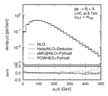
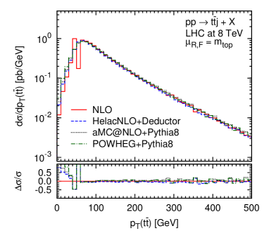
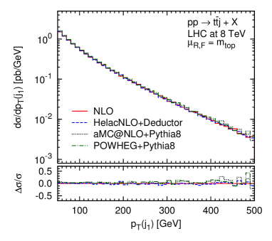
Figure 5: Differential distributions for $t\bar{t}j$ production. Comparison between NLO and several NLO+PS predictions.

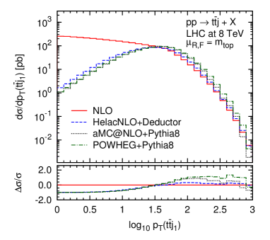
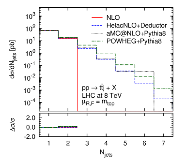
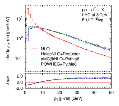
Figure 6: Differential distributions for $t\bar{t}j$ production. Comparison between NLO and several NLO+PS predictions.

We observe that distributions shown in Figure 5, which are not expected to be affected by showering effects have, to a good approximation, the same shape as at fixed order. The resummation effect is visible first and foremost in the transverse momentum distribution of the $t\bar{t}j$ system and other distributions shown in Figure 6. A more detailed analysis is presented in [72].

5 Conclusions

We have discussed recent progress towards matching next-to-leading QCD calculations for LHC processes with parton showers at next-to-leading logarithmic accuracy. Matched NLO+NLL calculations will provide accurate predictions for differential distributions and exclusive observables with experimental cuts, and are thus essential to fully exploit the potential of the upcoming LHC run.

To facilitate the matching of NLO calculations with parton showers, the subtraction terms needed to combine virtual and real corrections should by constructed from the splitting functions that define the parton shower. We have presented a subtraction scheme based on a parton shower with quantum interference and its implementation into the Helac-NLO software. The new subtraction scheme has been applied to a number of challenging processes, including the production of up to four heavy quarks at the LHC. The new scheme performs well compared to established methods. It not only provides an important internal check of multi-parton NLO calculations, but also forms the basis of current work on parton shower matching at NLL accuracy.

First results of such a new NLO+NLL calculation have been presented. We find that the resummation is important for a wide range of phenomenologically relevant distributions. Work is in progress to further improve on the accuracy of the calculation by adding sub-leading color effects and spin correlations.

References

- [1] M. Dobbs, “Incorporating next-to-leading order matrix elements for hadronic diboson production in showering event generators,” Phys. Rev. D 64 (2001) 034016.
- [2] J. Collins, “Monte-Carlo event generators at NLO,” Phys. Rev. D 65 (2002) 094016.
- [3] Y. j. Chen, J. Collins and X. m. Zu, “NLO corrections in MC event generator for angular distribution of Drell-Yan lepton pair production,” JHEP 0204 (2002) 041.
- [4] S. Frixione and B. R. Webber, “Matching NLO QCD computations and parton shower simulations,” JHEP 0206 (2002) 029.
- [5] Y. Kurihara, J. Fujimoto, T. Ishikawa, K. Kato, S. Kawabata, T. Munehisa and H. Tanaka, “QCD event generators with next-to-leading order matrix elements and parton showers,” Nucl. Phys. B 654 (2003) 301.
- [6] M. Krämer and D. E. Soper, “Next-to-leading order QCD calculations with parton showers. I: Collinear singularities,” Phys. Rev. D 69 (2004) 054019.
- [7] S. Frixione, P. Nason and B. R. Webber, “Matching NLO QCD and parton showers in heavy flavor production,” JHEP 0308 (2003) 007.
- [8] D. E. Soper, “Next-to-leading order QCD calculations with parton showers. II: Soft singularities,” Phys. Rev. D 69 (2004) 054020.
- [9] P. Nason, “A new method for combining NLO QCD with shower Monte Carlo algorithms,” JHEP 0411 (2004) 040.
- [10] Z. Nagy and D. E. Soper, “Matching parton showers to NLO computations,” JHEP 0510 (2005) 024.
- [11] C. W. Bauer and M. D. Schwartz, “Event generation from effective field theory,” Phys. Rev. D 76 (2007) 074004.
- [12] W. T. Giele, D. A. Kosower and P. Z. Skands, “A Simple shower and matching algorithm,” Phys. Rev. D 78 (2008) 014026.
- [13] S. Frixione, P. Nason and C. Oleari, “Matching NLO QCD computations with Parton Shower simulations: the POWHEG method,” JHEP 0711 (2007) 070.
- [14] C. W. Bauer, F. J. Tackmann and J. Thaler, “GenEvA. I. A New framework for event generation,” JHEP 0812 (2008) 010.
- [15] N. Lavesson and L. Lonnblad, “Extending CKKW-merging to One-Loop Matrix Elements,” JHEP 0812 (2008) 070.
- [16] S. Hoeche, F. Krauss, M. Schonherr and F. Siegert, “A critical appraisal of NLO+PS matching methods,” JHEP 1209 (2012) 049.
- [17] S. Frixione and B. R. Webber, “The MC@NLO 3.4 Event Generator,” arXiv:0812.0770 [hep-ph].
- [18] S. Alioli, P. Nason, C. Oleari and E. Re, “A general framework for implementing NLO calculations in shower Monte Carlo programs: the POWHEG BOX,” JHEP 1006 (2010) 043.
- [19] T. Gleisberg, S. Hoeche, F. Krauss, M. Schonherr, S. Schumann, F. Siegert and J. Winter, “Event generation with SHERPA 1.1,” JHEP 0902 (2009) 007.
- [20] J. Alwall, R. Frederix, S. Frixione, V. Hirschi, F. Maltoni, O. Mattelaer, H.-S. Shao and T. Stelzer et al., “The automated computation of tree-level and next-to-leading order differential cross sections, and their matching to parton shower simulations,” JHEP 1407, 079 (2014).
- [21] S. Gieseke, P. Stephens and B. Webber, “New formalism for QCD parton showers,” JHEP 0312 (2003) 045.
- [22] T. Sjostrand and P. Z. Skands, “Transverse-momentum-ordered showers and interleaved multiple interactions,” Eur. Phys. J. C 39 (2005) 129.
- [23] Z. Nagy and D. E. Soper, “Parton showers with quantum interference,” JHEP 0709 (2007) 114.
- [24] M. Dinsdale, M. Ternick and S. Weinzierl, “Parton showers from the dipole formalism,” Phys. Rev. D 76 (2007) 094003.
- [25] S. Schumann and F. Krauss, “A Parton shower algorithm based on Catani-Seymour dipole factorisation,” JHEP 0803 (2008) 038.
- [26] Z. Nagy and D. E. Soper, “Parton showers with quantum interference: leading color, spin averaged,” JHEP 0803 (2008) 030.
- [27] Z. Nagy and D. E. Soper, “Parton showers with quantum interference: leading color, with spin,” JHEP 0807 (2008) 025.
- [28] Z. Nagy and D. E. Soper, “Final state dipole showers and the DGLAP equation,” JHEP 0905 (2009) 088.
- [29] P. Z. Skands and S. Weinzierl, “Some remarks on dipole showers and the DGLAP equation,” Phys. Rev. D 79 (2009) 074021.
- [30] S. Platzer and S. Gieseke, “Coherent Parton Showers with Local Recoils,” JHEP 1101 (2011) 024.
- [31] Z. Nagy and D. E. Soper, “On the transverse momentum in Z-boson production in a virtuality ordered parton shower,” JHEP 1003 (2010) 097.
- [32] Z. Nagy and D. E. Soper, “Parton shower evolution with subleading color,” JHEP 1206 (2012) 044.
- [33] A. J. Larkoski, J. J. Lopez-Villarejo and P. Skands, “Helicity-Dependent Showers and Matching with VINCIA,” Phys. Rev. D 87 (2013) 5, 054033.
- [34] L. Hartgring, E. Laenen and P. Skands, “Antenna Showers with One-Loop Matrix Elements,” JHEP 1310 (2013) 127.
- [35] Z. Nagy and D. E. Soper, “A parton shower based on factorization of the quantum density matrix,” JHEP 1406 (2014) 097.
- [36] Z. Nagy and D. E. Soper, “Ordering variable for parton showers,” JHEP 1406 (2014) 178.
- [37] Z. Nagy and D. E. Soper, “Parton distribution functions in the context of parton showers,” JHEP 1406 (2014) 179.
- [38] G. Bevilacqua, M. Czakon, M. Kubocz and M. Worek, “Complete Nagy-Soper subtraction for next-to-leading order calculations in QCD,” JHEP 1310 (2013) 204.
- [39] M. Czakon, “A novel subtraction scheme for double-real radiation at NNLO,” Phys. Lett. B 693 (2010) 259.
- [40] C. H. Chung, M. Krämer and T. Robens, “An alternative subtraction scheme for next-to-leading order QCD calculations,” JHEP 1106 (2011) 144.
- [41] C. -H. Chung and T. Robens, “Nagy-Soper subtraction scheme for multiparton final states,” Phys. Rev. D 87 (2013) 074032.
- [42] T. Robens, “Nagy-Soper subtraction: a review,” Mod. Phys. Lett. A, Vol. 28, No. 23 (2013) 1330020.
- [43] S. Catani, M. H. Seymour, “A General algorithm for calculating jet cross-sections in NLO QCD,” Nucl. Phys. B 485 (1997) 291 [Erratum-ibid. B 510 (1998) 503].
- [44] S. Catani, S. Dittmaier, M. H. Seymour, Z. Trocsanyi, “The Dipole formalism for next-to-leading order QCD calculations with massive partons,” Nucl. Phys. B 627 (2002) 189.
- [45] M. Czakon, C. G. Papadopoulos, M. Worek, “Polarizing the Dipoles,” JHEP 0908 (2009) 085.
- [46] G. Bevilacqua, M. Czakon, M. V. Garzelli, A. van Hameren, A. Kardos, C. G. Papadopoulos, R. Pittau, M. Worek, “Helac-NLO,” Comput. Phys. Commun. 184 (2013) 986.
- [47] C. G. Papadopoulos and M. Worek, “Multi-parton cross sections at hadron colliders,” Eur. Phys. J. C 50 (2007) 843.
- [48] G. Bevilacqua, M. Czakon, C. G. Papadopoulos, R. Pittau and M. Worek, “Assault on the NLO Wishlist: ,” JHEP 0909 (2009) 109.
- [49] A. van Hameren, C. G. Papadopoulos, R. Pittau, “Automated one-loop calculations: A Proof of concept,” JHEP 0909 (2009) 106.
- [50] M. Cacciari, G. P. Salam, G. Soyez, “The Anti-k(t) jet clustering algorithm,” JHEP 0804 (2008) 063.
- [51] H. -L. Lai, M. Guzzi, J. Huston, Z. Li, P. M. Nadolsky, J. Pumplin and C. -P. Yuan, “New parton distributions for collider physics,” Phys. Rev. D 82 (2010) 074024.
- [52] J. Dai, J. F. Gunion, R. Vega, “Detection of neutral MSSM Higgs bosons in four b final states at the Tevatron and the LHC: An update,” Phys. Lett. B 387 (1996) 801.
- [53] M. J. Strassler, K. M. Zurek, “Echoes of a hidden valley at hadron colliders,” Phys. Lett. B 651 (2007) 374.
- [54] G. Bevilacqua, M. Czakon, M. Krämer, M. Kubocz and M. Worek, “Quantifying quark mass effects at the LHC: A study of at next-to-leading order,” JHEP 1307 (2013) 095.
- [55] R. M. Barnett, H. E. Haber, D. E. Soper, “Ultra-heavy Particle Production from Heavy Partons at Hadron Colliders,” Nucl. Phys. B 306 (1988) 697.
- [56] N. Greiner, A. Guffanti, T. Reiter, J. Reuter, “NLO QCD corrections to the production of two bottom-antibottom pairs at the LHC,” Phys. Rev. Lett. 107 (2011) 102002.
- [57] G. Bevilacqua and M. Worek, “Constraining BSM Physics at the LHC: Four top final states with NLO accuracy in perturbative QCD,” JHEP 1207 (2012) 111.
- [58] G. Ossola, C. G. Papadopoulos, R. Pittau, “CutTools: A Program implementing the OPP reduction method to compute one-loop amplitudes,” JHEP 0803 (2008) 042.
- [59] G. Ossola, C. G. Papadopoulos, R. Pittau, “Reducing full one-loop amplitudes to scalar integrals at the integrand level,” Nucl. Phys. B 763 (2007) 147.
- [60] G. Ossola, C. G. Papadopoulos, R. Pittau, “On the Rational Terms of the one-loop amplitudes,” JHEP 0805 (2008) 004.
- [61] P. Mastrolia, G. Ossola, C. G. Papadopoulos, R. Pittau, “Optimizing the Reduction of One-Loop Amplitudes,” JHEP 0806 (2008) 030.
- [62] P. Draggiotis, M. V. Garzelli, C. G. Papadopoulos, R. Pittau, “Feynman Rules for the Rational Part of the QCD 1-loop amplitudes,” JHEP 0904 (2009) 072.
- [63] A. van Hameren, “OneLOop: For the evaluation of one-loop scalar functions,” Comput. Phys. Commun. 182 (2011) 2427.
- [64] A. Kanaki, C. G. Papadopoulos, “Helac: A Package to compute electroweak helicity amplitudes,” Comput. Phys. Commun. 132 (2000) 306.
- [65] C. G. Papadopoulos, “Phegas: A Phase space generator for automatic cross-section computation,” Comput. Phys. Commun. 137 (2001) 247.
- [66] A. Cafarella, C. G. Papadopoulos, M. Worek, “Helac-Phegas: A Generator for all parton level processes,” Comput. Phys. Commun. 180 (2009) 1941.
- [67] A. van Hameren, “Kaleu: A General-Purpose Parton-Level Phase Space Generator,” arXiv:1003.4953 [hep-ph].
- [68] A. van Hameren, “Parni for importance sampling and density estimation,” Acta Phys. Polon. B 40 (2009) 259.
- [69] J. Beringer et al. [Particle Data Group Collaboration], “Review of Particle Physics (RPP),” Phys. Rev. D 86 (2012) 010001.
- [70] A. D. Martin, W. J. Stirling, R. S. Thorne, G. Watt, “Parton distributions for the LHC,” Eur. Phys. J. C 63 (2009) 189.
- [71] A. D. Martin, W. J. Stirling, R. S. Thorne, G. Watt, “Heavy-quark mass dependence in global PDF analyses and 3- and 4-color parton distributions,” Eur. Phys. J. C 70 (2010) 51.
- [72] M. Czakon, H. B. Hartanto, M. Kraus and M. Worek, “Matching the Nagy-Soper parton shower at next-to-leading order,” arXiv:1502.00925 [hep-ph].
- [73] T. Sjostrand, S. Mrenna and P. Z. Skands, “A Brief Introduction to PYTHIA 8.1,” Comput. Phys. Commun. 178 (2008) 852.
- [74] M. Bahr, S. Gieseke, M. A. Gigg, D. Grellscheid, K. Hamilton, O. Latunde-Dada, S. Platzer and P. Richardson et al., “Herwig++ Physics and Manual,” Eur. Phys. J. C 58 (2008) 639.
- [75] G. Corcella, I. G. Knowles, G. Marchesini, S. Moretti, K. Odagiri, P. Richardson, M. H. Seymour and B. R. Webber, “HERWIG 6: An Event generator for hadron emission reactions with interfering gluons (including supersymmetric processes),” JHEP 0101 (2001) 010.
- [76] T. Sjostrand, S. Mrenna and P. Z. Skands, “PYTHIA 6.4 Physics and Manual,” JHEP 0605 (2006) 026.
- [77] S. Platzer and M. Sjodahl, “Subleading improved Parton Showers,” JHEP 1207 (2012) 042.
- [78] F. Abe et al. [CDF Collaboration], “Evidence for color coherence in collisions at TeV,” Phys. Rev. D 50 (1994) 5562.
- [79] M. R. Whalley, D. Bourilkov and R. C. Group, “The Les Houches accord PDFs (LHAPDF) and LHAGLUE,” hep-ph/0508110.
- [80] S. Dittmaier, P. Uwer and S. Weinzierl, “NLO QCD corrections to t anti-t + jet production at hadron colliders,” Phys. Rev. Lett. 98 (2007) 262002.
- [81] S. Dittmaier, P. Uwer and S. Weinzierl, “Hadronic top-quark pair production in association with a hard jet at next-to-leading order QCD: Phenomenological studies for the Tevatron and the LHC,” Eur. Phys. J. C 59 (2009) 625.
- [82] K. Melnikov and M. Schulze, “NLO QCD corrections to top quark pair production in association with one hard jet at hadron colliders,” Nucl. Phys. B 840 (2010) 129.
- [83] K. Melnikov, A. Scharf and M. Schulze, “Top quark pair production in association with a jet: QCD corrections and jet radiation in top quark decays,” Phys. Rev. D 85 (2012) 054002.
- [84] S. Alioli, S. O. Moch and P. Uwer, “Hadronic top-quark pair-production with one jet and parton showering,” JHEP 1201 (2012) 137.
- [85] A. Kardos, C. Papadopoulos and Z. Trocsanyi, “Top quark pair production in association with a jet with NLO parton showering,” Phys. Lett. B 705 (2011) 76.